Deep Neural Network Architecture Search via Decomposition-Based Multi-Objective Stochastic Fractal Search

1  Introduction

With the rapid development of deep learning technique and computer hardware system, deep neural network has become one of the most popular and effective approaches in solving real-world problems, such as computer vision [1]. Compared with classical machine learning algorithms, an intuitive reason for the prominent performance is that almost network architectures are carefully designed professionally and fixedly, such as AlexNet [2], VGGNet [3], ResNet [4], RCNN [5] and DenseNet [6]. It is generally believed that a universal approach to enhancing the accuracy capabilities of deep neural networks is to expand the network deeper and wider [7]. However, more complicated network may lead to a dramatic increase in the number of candidate neural architectures and indispensable training and processing computational resource. This undoubtedly brings challenges to artificial network generation and modification. In addition, manually designed networks require a great deal of expertise and need to be redesigned and tuned when the problem changes.

Recently, Neural Architecture Search (NAS) has become an emerging and popular research area, since the engineering of this automated search-build network can easily overcome the above shortcomings. The NAS method first determines the search space with different types of layers and parameters. Then, a search strategy is usually specified to search for well-performing architectures. Specifically, Baker et al. [8] proposed a reinforcement learning based meta-modeling algorithm to automatically design convolutional neural network (CNN) architectures, called MetaQNN. Zoph et al. [9,10] proposed a NAS method with reinforcement learning and recurrent networks which optimizes the validation accuracy via policy gradients to generate the best neural architecture. Zhong et al. [11] proposed a block-wise network generation method using Q-learning and ε-greedy exploration, called BlockQNN. Each convolutional block in BlockQNN is represented with a directed acyclic graph, and the optimal blocks achieved are assembled into the whole CNN. The successful application of the augmented neuro evolution of topologies (NEAT) approach has made evolutionary algorithms (EAs) a popular choice for NAS search strategies [12–14]. Xie et al. [15] proposed GeNet to learn the structure of CNN through genetic algorithm automatically. Each neural structure is encoded by a fixed-length binary string and evaluated on the validation set. Liu et al. [12] proposed a hierarchical genetic representation, which selects the hierarchical unit with the best accuracy through underlying operations, and finally inserts it into a large CNN model. Wang et al. [14] used particle swarm optimization (PSO) and a novel encoding to search chain-structured CNNs. In Fernandes Junior et al. [16], a modified PSO is proposed with variable length particles and a novel velocity operator to search for an optimal CNN structure.

However, the above research regards NAS as a single-objective optimization problem, and the optimization goal is the accuracy performance of the network while ignoring the complexity of the network, including the number of parameters. Therefore, the discovered architectures are always overly complex networks, which contain a large number of redundant layer types and connections, which reduces the search efficiency and also makes the resulting architectures overly complex. To this end, Hsu et al. [17] proposed a reinforcement learning based multi-objective NAS method (MONAS). The network performance is evaluated by a weighted linear combination of prediction accuracy and computational cost. Tan et al. [18] further proposed an automated mobile NAS (MnasNet), in which a special weighting method is adopted to find multiple Pareto optimal solutions. More recently, Elsken et al. [19] proposed an EA-based multi-objective architecture search method, where the accuracy and parameters of the architecture are considered simultaneously. Jiang et al. [20] proposed the use of MOPSO/D to complete multi-objective NAS, called MOPSO/D-Net, using a multi-branch architecture to obtain an efficient architecture with fewer parameters.

A myriad of existing works reveal that it is necessary to consider multiple abilities when constructing neural network architecture, such as accuracy, complexity of the model and consumption of computational resources. Since these objectives are usually conflicting with each other, it is reasonable to formulate NAS as a multi-objective optimization problem (MOP). Multi-objective evolutionary algorithms (MOEAs) are a kind of effective methods to solve the MOP, and have been successfully applied in many practical problems. In MOEAs, the decomposition-based idea has received more and more attention due to its prominent performance in finding trade-off solutions, such as NSGAIII [21], MPSO/D [22] and RVEA [23]. In general, the MOP is decomposed into several subproblems using a set of reference vectors, and each of the subproblems is optimized based on stable neighborhood relations and efficient local matching.

Based on the discussion above, this paper proposes a novel NAS method called decomposition-based multi-objective stochastic fractal search (DMOSFS) algorithm. The key contributions of this paper are as follows:

(1) Our proposed algorithm targets both the training set accuracy of the architecture and the network structure complexity. The challenge of multi-objective search is to ensure solution diversity and convergence, and we use a decomposition-based strategy to search for architectures.

(2) In the proposed algorithm, a chained direct coding scheme with specific addition and subtraction rules is designed to represent the network architecture. Considering the discrete characteristic of the search space, the random fractal search step size is discretized to correspond to the structural peculiarity of the network architecture. Two offspring generation methods are used to improve the global and local search ability of the algorithm. On top of this, an information exchange mechanism between architectures is also presented to speed up convergence and intensify the search ability of the algorithm further.

(3) Experimental results show that the proposed DMOSFS outperforms single-objective NAS methods in terms of the achieved trade-off solutions. The DMOSFS also provides competitive results on six benchmark datasets, and excels in terms of both search speed, architecture accuracy and params.

In the remainder of this paper, we first briefly introduce some concepts and algorithmic ideas related to multi-objective optimization. Thereafter, in Section 3, we outline the procedure of our proposed DMOSFS in detail. The experimental design and results are presented in Section 4. Finally, the conclusion of the algorithm is drawn in Section 5.

2  Background

2.1 Basic Concepts

Generally, a MOP can be stated as:

minxf(x)=(f1(x),f2(x),⋯,fM(x))s.t.x∈X(1)

where X⊆Rn is the decision space with x=(x1,x2,⋯,xn) being the decision vector, fi is the objective functions to be optimized simultaneously, with i=1,⋯,M. Due to the constrains and conflict among the various objectives, it is impossible to find an ideal solution that achieving optima of each objective simultaneously so we can only find a series of compromise solutions to balance each goal as much as possible. These solutions are the trade-offs of various objectives which are also called Pareto optimal solutions. They are also called Pareto front (PF) in the objective space, and Pareto set (PS) in the decision space.

2.2 Stochastic Fractal Search

Stochastic Fractal Search (SFS) was first proposed by Salimi [24] in 2015. The core concept in SFS is “fractal” representing the property of an object or quantity which explains self-similarity on all scales. Diffusion Limited Aggregation (DLA) [25] is one of the most commonly used random fractals methods to generate fractal shape objects and is firstly applied in Fractal Search (FS) by Salimi. In SFS, a series of Gaussian walks are added to the diffusion process to create new particles and simulate the DLA method as follows:

GW1=Gaussian(μBP,σ)+(ε×BP−ε′×Pi)(2)

GW2=Gaussian(μp,σ)(3)

and

σ=|log⁡(t)t×(Pi−BP)|(4)

where ε and ε′ are random selected in interval [0, 1] with uniform distribution. BP and Pi represent the position of the best solution and the i-th solution in the population, respectively. The mean value μBP and μP of the two Gaussian distributions equals to the absolute value of the solution vector |BP| and |P|. The term log⁡(t)t is used to increase the distance of Gaussian walks as the iteration progresses.

2.3 Decomposition-Based Methods

The idea of decomposition was first proposed by Liu et al. [26], where a set of direction vectors are used to divide the whole PF into a series of parts, which is equivalent to dividing MOPs into an equal number of multi-objective sub-problems. In reality, a set of weight vectors are adopted to convert a MOP into a number of sub-problems by dividing the entire objective space into some subspaces, in which each sub-problem remains a MOP. Such a decomposition strategy has been taken seriously. In this paper, all reference vectors used are unit vectors with the initial point as the origin in the first quadrant. In order to generate a set of uniformly distributed reference vectors, we use the reference point generation method in [21].

3  The Proposed Approach

3.1 Network Architecture Representation

3.1.1 Architecture Encoding

When designing algorithms to deal with complex structures such as CNN architectures, encoding is first and foremost. We use a CNN architecture direct encoding scheme [16], which searches chained structures. Every time a CNN is used for training, testing, or evaluation, the model is compiled according to the type of each layer in the particle.

Using chain coding will from the corresponding block-based search space. In a chained representation, the architecture represented by each particle can be thought of as an accumulation of functional blocks allowing the use of custom blocks. The search space of the algorithm consists of six types of layers: convolutional layer, efficient channel attention block (ECA block) [27], basic-block module in ResNet [4], max pooling layer, average pooling layer and fully connected layer. Each position in the encoding structure contains information about the type and hyperparameters. In other words, a single position in the encoding includes not only the layer type but also the hyperparameters corresponding to that type, such as the number of output feature maps (if a convolutional layer) or the number of neurons (if a fully connected layer) and kernel size (if convolution). Fig. 1 illustrates an example of the encoding scheme, where CO, ECA, Res, PO, and FC represent convolutional layers, ECA blocks, basic-block modules in ResNet, pooling layers (maximum or average), and fully connected layers, respectively. The advantage of this chained encoding structure is that the calculation and compilation model can be directly performed according to the encoding information without conversion. The blocks used in this article are of the six-layer type shown earlier.

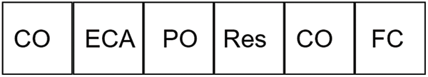
Figure 1: Single individual architecture representation

3.1.2 Architecture Operation Method

To calculate the growth step size of an individual, we need to specify the calculation rule between two individuals. In order to avoid the formation of a fully connected layer between the convolutional layer and the pooling layer (Conv/Pool), resulting in an invalid CNN architecture, each individual Conv/Pool and FC layer operates independently. During the architecture operation process, we only consider the layer type of each particle, independent of the hyperparameters. Additionally, the addition operation between individuals is modified according to the second addend, keeping the layer and corresponding hyperparameters of the second individual. For instance, if two individuals have different layer types at the same respective location, the first individual’s type is swapped for the second individual’s layer type. If both individuals have different layer types, the first individual’s layer and corresponding hyperparameters are retained as the result of the subtraction between individuals. For example, if two individuals have the same layer type, the difference will be zero. If the first individual has fewer layers than the second, –1 will be added to the final difference, indicating that the block at that position should be deleted. On the other hand, if the first individual has more layers than the second, the final difference will be added with +L, where L indicates the type of layer to be added, including CO, ECA, Res, PO, and FC.

3.2 Framework of DMOSF

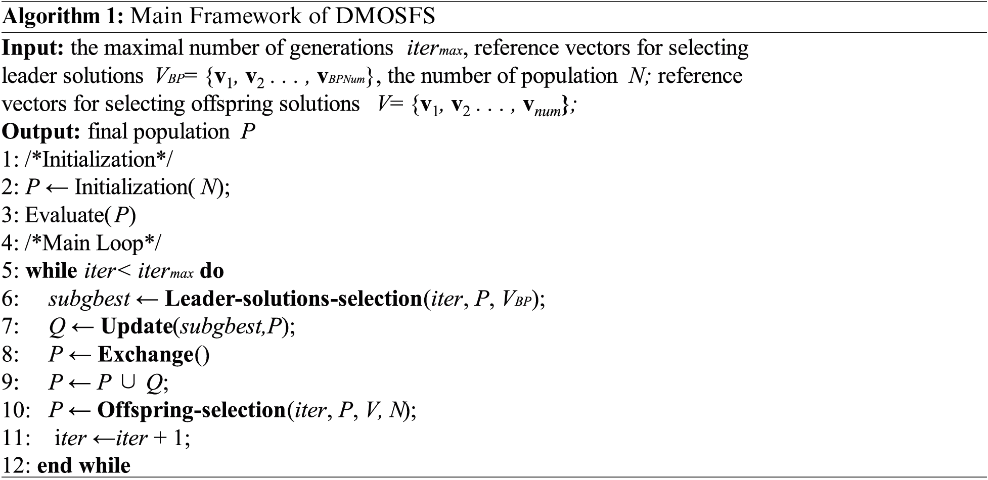
In contrast to the single-objective NAS method, we propose a decomposition-based multi-objective stochastic fractal search that considers both precision and complexity tradeoffs when discovering neural network architectures. Initially, a series of reference vectors decompose the target space into a set of subspaces. That is, uses a set of weight vectors to convert the MOP into multiple sub-problems, where each sub-problem is still an MOP. Considering the discrete nature of the search space, we discretize the stochastic fractal search step size so that the characteristics of the network architecture can be more effectively characterized by encoding. In the step size update stage, two different update methods are used to ensure the global and local search ability of the algorithm in the early stage and later stage, respectively. In addition, in order to further enhance the performance of the algorithm, an information exchange mechanism between architectures is designed. The main framework of the proposed DMOSFS is shown in Algorithm 1.

3.2.1 Population Initialization

In the initialization stage, N particles are created to represent different network architectures. Each particle generates a random number of layers, between three and lmax (the maximum number of layers). To ensure the resulting CNN architecture is feasible, the first layer of each particle is fixed as a convolutional layer or an ECA block, and the last layer is set as a fully connected layer. Additionally, fully connected layers (FC) can only be placed after other types of layers. Therefore, during initialization, the algorithm ensures that once an FC layer is added to the architecture, each subsequent layer is also an FC layer.

The initialization process consists of the following five layer-addition strategies:

-Convolution layer addition mechanism: adds a convolution layer with a random number of output feature maps (between 1 and mapsmax) and kernel size (between 3 × 3 and kmax × kmax, with a step size of 1 × 1), where mapsmax represents the maximum number of channels of the output feature map, and kmax represents the maximum convolution kernel size.

-ECA block addition mechanism: adds an ECA block with global average pooling for each channel separately and followed by two 1 × 1 convolutional layers. The sigmoid function was used for generating the channel weights.

-Residual block addition mechanism: adds a basic residual block, including skip connections.

-Pooling layer addition mechanism: adds a max pooling layer or an average pooling layer with a size of 3 × 3 and a stride of 2 × 2 randomly.

-Fully connected layer addition mechanism: adds a fully connected layer with a random number of neurons between 1 and the maximum nmax. All layers use the rectified linear unit (ReLU) activation function.

It is worth mentioning that the number of pooling layers is limited by the size of the input data, because too many pooling layers can result in a feature map size of 0.

3.2.2 Fitness Assessment

After initialization, each particle architecture will be compiled into a complete CNN by decoding and eevaluate training to obtain the model training accuracy and the number of model parameters contemporary. In this work, we use Adam [28] for training and Xavier to initialize the weights. In addition, dropout and batch normalization can be added between layers to avoid the overfitting problem [29].

3.2.3 Particle Update

In the DMOSFS algorithm, the step size of any given particle (P) is adjusted based on the difference with the subspace leader solution (subgbest). In the following, the selection of the leader solution subgbest and the step determination strategy will be explained, respectively.

A.   Selection of leader solution in subpopulation

The reference vectors divide the objective space into multiple subspaces, and a leader solution is selected in each subspace to assist the generation of solutions in this subspace, which can better balance the convergence and diversity of the algorithm.

Firstly, we transform the objective values of each particle by subtracting the minimum value to ensure that all transformed objective values are in the first quadrant. After that, the population is divided into N subpopulations according to the spatial relationship of each solution with the reference vector. In each subpopulation, a leader solution (subgbest) is selected using the angle-penalized distance (APD) [23] as the selected standard:

dt,i,j=‖ft,i′‖⋅(1+M⋅(ttmax)α⋅θt,i,jφvt,j)(5)

and

φvt,j=minl∈{1,…,N},l≠j‖vt,j,vt,l‖(6)

where M is the number of objectives, t and tmax are the t-th generation and the maximum number of generations, respectively. N is the number of reference vectors, φvt,j is the angle between the reference vector vt,j and the other reference vector closest to it. The solution with the smallest APD in each subpopulation is selected as the leader solution.

B.   Step size determination

With the subgbest selected in each subpopulation, we using the following method to update the step size:

{(BP−P)(j) unchangedr<d(BP−P)(j) randomadjustmentelse(7)

where j represents the j-th layer of the network structure, and d is the randomized control parameter of the algorithm. A larger d will help the particle structure converge to the global optimum structure more quickly, but may reduce the probability of escaping from a local optimum. In contrast, smaller values of d will reduce the diversity of the population, increasing the likelihood of getting stuck in a locally optimal architecture. From this equation, whether to keep the j-th layer unchanged or randomly initialized to other block types for replacement depends on the value of r, which is calculated according to the following formula:

{r=Gaus(0,1−iteritermax)p<(iteritermax)1/3r=Levy(β)else(8)

where β is set to 1.5, and p is a random number generated in [0, 1). The benefit of using two different methods to generate r is that a larger r can be obtained through Levy flight in the early search stage to enhance the global exploration ability of the algorithm by randomly adjusting the step size.

Once the stride calculation is complete, the algorithm adds or removes corresponding layers from the architecture according to the stride. It is important to note that we need to check the number of pooling layers in the architecture to decide whether to remove a pooling layer. In other words, if the related architecture of the particle has more pooling layers than allowed, the excess pooling layers are removed from back to front.

3.2.4 Information Exchange

In DMOSFS, an information exchange mechanism between architectures is designed to further improve the search ability of the algorithm. Information is exchanged by bit, that is, exchange between layers of different architectures after updating.

Pi'(j)=Pt(j)−Pi(j)(9)

where Pt is the t-th individual randomly selected in the population, and j represents the j-th layer of the individual. The condition of exchange is:

{Pi<(iteritermax)1/3Pi(j)<(iteritermax)1/3(10)

Information exchange can only be performed when individual Pi and the j-th layer Pi(j) satisfy the exchange submission at the same time. Through this constraint, the algorithm can exchange more information in the early stage to increase the search ability.

3.2.5 Offspring Selection

We adopt an elitist strategy to select offspring from the updated solution and the parent population to the next generation. Offspring in each subspace is selected independently based on the distance measurement. Due to the non-uniform distribution of solutions, not enough solutions can be selected. To ensure the distribution of solutions, we propose the circular selection mechanism.

Initially, the objective values F={f1,…,f|P|} of the individuals are converted to F' = { f1',...,f| P |' }:

f1'=fi−zi,min(11)

where i=1,…,|P|, zmin={z1,min,…,zM,min} represents the minimum value on each objective in the population, M is the number of objectives.

After completing the transformation of the objective values, we divide the solutions into different subspaces according to the spatial relationship between the solutions and the reference vectors. In this way, a solution fi is assigned to a subpopulation Pk if and only if the cosine value between f1' and vk is the maximum among all the reference vectors:

Pk={fi|k=argmaxj∈{1,⋯,N}cos⁡θi,j}(12)

where fi represents the i-th particle in P, with i=1,…,|P|, cos⁡θi,j is the cosine value between the converted solution f1' and the reference vector vj.

Since the number of subspaces is close to the number of individuals in each generation population, the uniformity of the distribution of selected solutions is maintained to satisfy the diversity of solutions. To better select solutions with sufficient convergence, we use the Euclidean distance as the selection criterion:

di=‖f1′‖(13)

where ‖⋅‖ represents Euclidean norm. According to the distance calculated by formula (13), the solution of the minimum distance in each subpopulation is selected as the next generation solution.

On account of the uneven distribution of solutions, not every subpopulation has candidate solutions. To solve this, we adopt circular selection to obtain enough candidate solutions. Specifically, an optimal solution is selected from each subpopulation according to the selection criteria in the order of the reference vectors. If the selected solutions are not enough, repeat the above process until enough solutions are selected.

4  Comparative Studies

The performance of the proposed DMOSFS was tested on a set of classic image classification datasets. The following subsections will describe the datasets, comparative models, algorithm parameters, and experimental results in detail.

4.1 Benchmark Test Datasets

To evaluate the proposed algorithm and compare the performance with other deep learning models, we selected six datasets with publicly available results: MNIST, MNIST-RD, MNIST-RB, MNIST-RD + BI, Rectangles, and Convex. Due to limited computing power and the aim of developing scalable and efficient search algorithms, we only tested our algorithm on datasets with small input sizes. The configuration of these datasets is summarized in Table 1.

The MNIST [30] dataset is a standard benchmark for testing new machine learning algorithms. MNIST-RD (rotated digits), MNIST-RB (random noise as background), and MNIST-RD + BI (rotated digits and background images) were modified from the original MNIST by Larochelle et al. [31]. These datasets contain irrelevant information compared to the original MNIST, making it a good test of the model’s generalization ability. The modified datasets also have a small number of training samples, which poses a challenge to the model.

The Rectangles dataset consists of black and white images of rectangles with different widths and heights. The motivation is to learn which dimension is greater, the width or the height. The Convex dataset contains black and white images of geometric shapes, and the objective is to determine whether the shape is convex or not.

4.2 Compared Algorithms

To evaluate the performance of our proposed DMOSFS algorithm, we compared the results with those of state-of-the-art deep learning algorithms. The comparing algorithms include population-based algorithms such as evoCNN [32], IPPSO [14], psoCNN [16], and MOPSO/D-Net [20], which are similar to the proposed DMOSFS in that individuals evolve over time to find a suitable CNN model for the corresponding dataset. We also select some manually-designed deep learning models for comparison.

For the MNIST dataset, we selected more advanced CNNs for comparison, including artificially designed networks such as RCNN [5], DropConnect [33], ResNet [4], CapsNet [34], and LeNet-5 [35], as well as automatically designed networks like evoCNN, IPPSO, psoCNN, MnasNet [18], GeNet [15], and MOPSO/D-Net. We also compared the architecture accuracy results obtained by applying SFS to single-target NAS (called SFSCNN) according to our encoding method and particle update method.

For the MNIST-RD, MNIST-RB, MNIST-RD + BI, Rectangles, and Convex datasets, we selected CAE-1 [36], CAE-2 [36], PCANet-2 [37], RandNet-2 [37], LDANet-2 [37], evoCNN, IPPSO, psoCNN, and SFSCNN as comparison models.

4.3 Algorithm Parameters

In this section, the comparison results by the DMOSFS algorithm and other deep learning algorithms are given. In the experiments, DMOSFS was tested on a single Nvidia TITAN Xp GPU with 12 GB of display memory. The parameters used in DMOSFS can be divided into three categories: algorithm optimization parameters, CNN architecture initialization parameters and CNN training parameters. The values of the parameters are given in Table 2.

4.4 Experimental Results

Fig. 2 presents the performance of the Pareto optimal solutions obtained by DMOSFS after 20 generations on the training data set. The non-dominated solutions achieved are limited, while more are needed in the training process. During the search process of DMOSFS, we keep 20 solutions in each generation even if some of them are dominated by others. The accuracy of the training set and the number of model parameters are the two evaluation indicators of the multi-objective NAS we built. As shown in Fig. 2, the Pareto front obtained on each data set progressively approximates the optimal direction of each objective. The trade-off solution achieves a relatively small validation error rate and fewer parameters than the initial generation. It is attributed to the search process of the two targets in the reference vector-based multi-target SFS. During this process, solutions far from reference vectors or have large scalar values are discarded, promoting solution convergence and indicating the algorithm’s effectiveness on both objectives. Moreover, due to the decomposition-based search, the final solutions exhibit good diversity in the target space, as evidenced by their uniform distribution. This approach avoids the absence of boundary solutions while retains more reasonable candidates throughout the evolution process, making it easier for users to choose the most suitable solution for their needs. The performance of the Pareto solutions on the test data sets is depicted in Fig. 3.

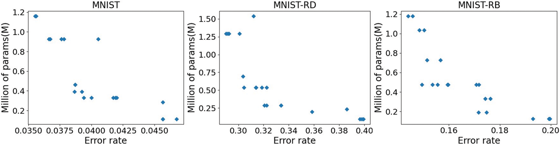
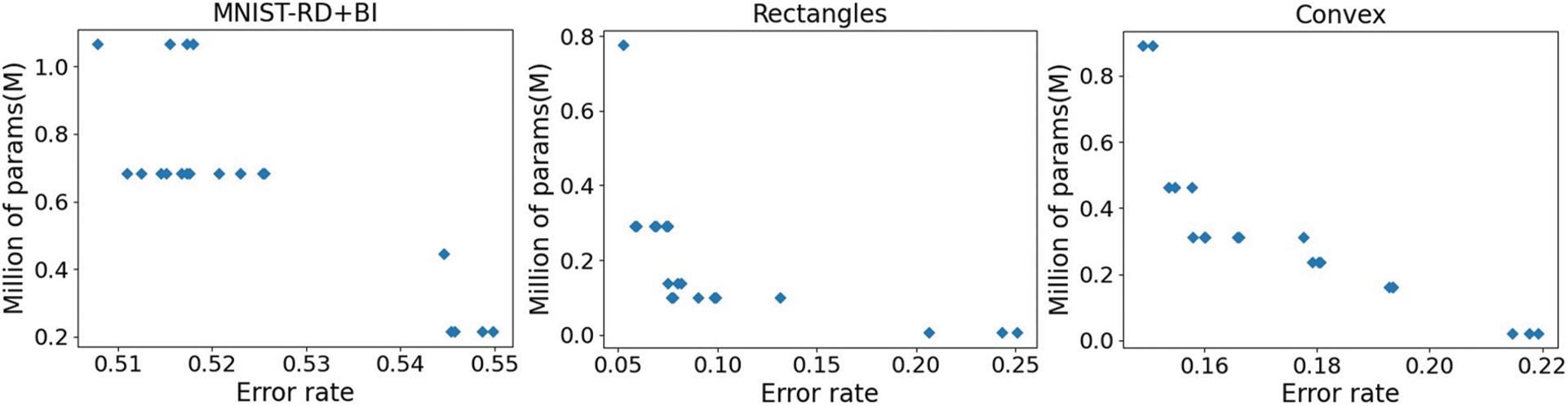
Figure 2: Performance of the final particles obtained by DMOSFS on the training datasets

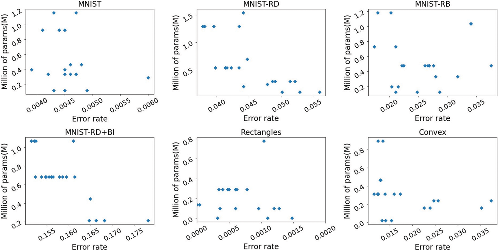
Figure 3: Performance of the final particles obtained by DMOSFS on the test datasets

In practice, it is necessary to choose an appropriate solution from the Pareto front obtained by DMOSFS. According to prior knowledge, the architecture with the highest classification accuracy on the test set is selected. Table 3 presents the detained layer composition of the best architectures for different datasets. Notably, the algorithm tends to employ a single fully connected layer at the end of each CNN. This has been verified by previous research, which suggests that a single fully connected layer yields better results than multiple fully connected layers [38]. The number of layers in the neural network architecture varies across problems, demonstrating that the variable-length encoding method is more flexible and provides more search possibilities. Each architecture contains at least one residual block, highlighting the strong performance of the residual block in feature extraction.

The comparison results of the CNNs discovered by DMOSFS with manual and automatic models on the MNIST dataset are summarized in Table 4. From the table, DMOSFS achieved higher test accuracy than CAE-1, CAE-2, PCANet-2, RandNet-2, LDANet-2, LeNet-5, and ResNet. It also approached the state-of-the-art results of CapsNet, RCNN, and DropConnect, which usually rely on special techniques that are excluded from the search space of NAS methods. Apart from handcrafted models, DMOSFS outperformed five automated models of evoCNN, IPPSO, psoCNN, MnasNet, and MOPSO/D-Net. It also achieved the same error rate as GeNet, the best among the selected comparison models. In terms of structural complexity, the proposed algorithm yielded more compact and efficient CNNs, with 0.39 M parameters, which is slightly higher than MOPSO/D-Net, less than LeNet-5, 4× fewer than IPPSO, 6× fewer than SFSCNN, 8× fewer than psoCNN, and 9× fewer than MnasNet.

It is also demonstrated in Table 4 that the proposed DMOSFS has the least computational cost. Although our accuracy is consistent with GeNet, GeNet requires expensive computing resources (more than 24 h on multiple GPUs), which may be its attempt to search a complete architecture. IPPSO, psoCNN, and SFSCNN complete the task in 2.5 h on 2 GPUs, 7.3 h on 1 GPU, and 4.3 h on 1 GPU, respectively. These three methods use automated chain structures and shallow architectures to make training easier and fitness evaluation faster. MOPSO/D-Nets uses a chain structure and multi-branch architecture, which can further reduce the search time to 6 h on a single GPU. But DMOSFS only needs 3.4 h on a single GPU, which is the least consumption in the comparison algorithms. This is probably because we are using a chained structure. The results demonstrate that DMOSFS search can make the searched architectures more accurate, with fewer parameters and less cost.

Table 5 shows the comparison of the architecture obtained by DMOSFS on the other five datasets. On the Rectangles and Convex datasets, DMOSFS performs best showing that the algorithm can find a network architecture with sufficient accuracy. The accuracy performance on MNIST-RB is second only to SFSCNN and outperforms other models. The accuracy performance on the remaining two datasets is not as good as SFSCNN and psoCNN, but still better than other algorithm models. It is worth noting that the accuracy results of SFSCNN on MNIST-RD, MNIST-RB, MNIST-RD + BI, and Rectangles are all the best. These results can prove the superiority of the step update method and information exchange in our proposed algorithm. DMOSFS does not perform as well as SFSCNN because the number of iterations of DMOSFS is very small in consideration of the computational cost. When the number of iterations is increased, the performance will become better.

In terms of model complexity, DMOSFS has fewer parameters (1.29, 0.7, 1.06, 1.38, and 0.3 M) compared to psoCNN and SFSCNN. Overall, we can derive that the proposed DMOSFS can effectively search for the efficient and simple neural network architectures with a lower computational cost.

5  Conclusion

In this work, we propose a decomposition-based multi-objective stochastic fractal search NAS method. The method considers two conflicting goals, model accuracy, and parameters, and finally obtains a high-performance and compact CNN with a small search cost. To effectively represent the network architecture, we use a chained direct encoding scheme and discretize the stochastic fractal search step size to optimize the network architecture more effectively. A set of reference vectors are also adopted to assist in the update and selection of offspring, maintaining the performance and diversity of the obtained architecture, and building an efficient search space that can achieve competitive results compared with hand-crafted and automatically generated CNNs. Our results demonstrate that DMOSFS can quickly find CNN architectures with high accuracy and few parameters for the given dataset. The model obtained by DMOSFS is superior in accuracy and complexity and uses less search cost compared to other methods.

In future work, Firstly, we consider adding parallel connections to the encoding method to improve the search performance and obtain more complex models. Then add more complex basic blocks in the search space, thereby reducing the number of parameters and improving model accuracy.

Acknowledgement: The authors would like to thank the editors and all the anonymous reviewers for their valuable comments and suggestions.

Funding Statement: This work was supported by the China Postdoctoral Science Foundation Funded Project (Grant Nos. 2017M613054 and 2017M613053), the Shaanxi Postdoctoral Science Foundation Funded Project (Grant No. 2017BSHYDZZ33) and the National Science Foundation of China (Grant No. 62102239).

Author Contributions: Study conception and design: Hongshang Xu, Bei Dong; data collection: Xiaochang Liu; analysis and interpretation of results: Hongshang Xu, Bei Dong, Xiaojun Wu; draft manuscript preparation: Hongshang Xu. Bei Dong. All authors reviewed the results and approved the final version of the manuscript.

Availability of Data and Materials: Data will be made available on request.

Conflicts of Interest: The authors declare that they have no conflicts of interest to report regarding the present study.

References

1. J. Schmidhuber, “Deep learning in neural networks: An overview,” Neural Networks, vol. 61, pp. 85–117, 2015. [Google Scholar] [PubMed]

2. A. Krizhevsky, I. Sutskever and G. E. Hinton, “Imagenet classification with deep convolutional neural networks,” Communications of the ACM, vol. 60, no. 6, pp. 84–90, 2017. [Google Scholar]

3. K. Simonyan and A. Zisserman, “Very deep convolutional networks for large-scale image recognition,” arXiv preprint arXiv:1409.1556, 2014. [Google Scholar]

4. K. He, X. Zhang, S. Ren and J. Sun, “Deep residual learning for image recognition,” in 2016 IEEE Conf. on Computer Vision and Pattern Recognition (CVPR), Las Vegas, NV, USA, pp. 770–778, 2016. [Google Scholar]

5. M. Liang and X. Hu, “Recurrent convolutional neural network for object recognition,” in 2015 IEEE Conf. on Computer Vision and Pattern Recognition (CVPR), Boston, MA, pp. 3367–3375, 2015. [Google Scholar]

6. G. Huang, Z. Liu, L. van der Maaten and K. Weinberger, “Densely connected convolutional networks,” in 2017 IEEE Conf. on Computer Vision and Pattern Recognition (CVPR), Honolulu, HI, USA, pp. 2261–2269, 2017. [Google Scholar]

7. C. Szegedy, W. Liu, Y. Jia, P. Sermanet, S. Reed et al., “Going deeper with convolutions,” in 2015 IEEE Conf. on Computer Vision and Pattern Recognition (CVPR), Boston, MA, USA, pp. 1–9, 2015. [Google Scholar]

8. B. Baker, O. Gupta, N. Naik and R. Raskar, “Designing neural network architectures using reinforcement learning,” arXiv preprint arXiv:1611.02167, 2016. [Google Scholar]

9. B. Zoph and Q. V. Le, “Neural architecture search with reinforcement learning,” arXiv preprint arXiv:1611.01578, 2016. [Google Scholar]

10. B. Zoph, V. Vasudevan, J. Shlens and Q. Le, “Learning transferable architectures for scalable image recognition,” in 2018 IEEE/CVF Conf. on Computer Vision and Pattern Recognition (CVPR), Salt Lake City, UT, USA, pp. 8697–8710, 2018. [Google Scholar]

11. Z. Zhong, J. Yan, W. Wu, J. Shao and C. L. Liu, “Practical block-wise neural network architecture generation,” in 2018 IEEE/CVF Conf. on Computer Vision and Pattern Recognition, Salt Lake City, UT, USA, pp. 2423–2432, 2018. [Google Scholar]

12. H. Liu, K. Simonyan, O. Vinyals, C. Fernando and K. Kavukcuoglu, “Hierarchical representations for efficient architecture search,” arXiv preprint arXiv:1711.00436, 2017. [Google Scholar]

13. E. Real, S. Moore, A. Selle, S. Saxena, Y. L. Suematsu et al., “Large-scale evolution of image classifiers,” in Int. Conf. on Machine Learning, Sydney, Australia, PMLR, pp. 2902–2911, 2017. [Google Scholar]

14. B. Wang, Y. Sun, B. Xue and M. Zhang, “Evolving deep convolutional neural networks by variable-length particle swarm optimization for image classification,” in 2018 IEEE Congress on Evolutionary Computation (CEC), Rio de Janeiro, Brazil, pp. 1–8, 2018. [Google Scholar]

15. L. Xie and A. Yuille, “Genetic CNN,” in 2017 IEEE Int. Conf. on Computer Vision (ICCV), Venice, Italy, pp. 1388–1397, 2017. [Google Scholar]

16. F. E. Fernandes Junior and G. G. Yen, “Particle swarm optimization of deep neural networks architectures for image classification,” Swarm and Evolutionary Computation, vol. 49, pp. 62–74, 2019. [Google Scholar]

17. C. H. Hsu, S. H. Chang, J. H. Liang, H. P. Chou, C. H. Liu et al., “Monas: Multi-objective neural architecture search using reinforcement learning,” arXiv preprint arXiv:1806.10332, 2018. [Google Scholar]

18. M. Tan, B. Chen, R. Pang, V. Vasudevan, M. Sandler et al., “MnasNet: Platform-aware neural architecture search for mobile,” in 2019 IEEE/CVF Conf. on Computer Vision and Pattern Recognition (CVPR), Long Beach, CA, USA, pp. 2815–2823, 2019. [Google Scholar]

19. T. Elsken, J. H. Metzen and F. Hutter, “Efficient multi-objective neural architecture search via lamarckian evolution,” arXiv preprint arXiv:1804.09081, 2018. [Google Scholar]

20. J. Jiang, F. Han, Q. Ling, J. Wang, T. Li et al., “Efficient network architecture search via multiobjective particle swarm optimization based on decomposition,” Neural Networks, vol. 123, pp. 305–316, 2020. [Google Scholar] [PubMed]

21. K. Deb and H. Jain, “An evolutionary many-objective optimization algorithm using reference-point-based nondominated sorting approach, part I: Solving problems with box constraints,” IEEE Transactions on Evolutionary Computation, vol. 18, no. 4, pp. 577–601, 2014. [Google Scholar]

22. C. Dai, Y. Wang and M. Ye, “A new multi-objective particle swarm optimization algorithm based on decomposition,” Information Sciences, vol. 325, pp. 541–557, 2015. [Google Scholar]

23. R. Cheng, Y. Jin, M. Olhofer and B. Sendhoff, “A reference vector guided evolutionary algorithm for many-objective optimization,” IEEE Transactions on Evolutionary Computation, vol. 20, no. 5, pp. 773–791, 2016. [Google Scholar]

24. H. Salimi, “Stochastic fractal search: A powerful metaheuristic algorithm,” Knowledge-Based Systems, vol. 75, pp. 1–18, 2015. [Google Scholar]

25. T. A. Witten and L. M. Sander, “Diffusion-limited aggregation,” Physical Review B, vol. 27, no. 9, pp. 5686, 1983. [Google Scholar]

26. H. L. Liu, F. Gu and Q. Zhang, “Decomposition of a multiobjective optimization problem into a number of simple multiobjective subproblems,” IEEE Transactions on Evolutionary Computation, vol. 18, no. 3, pp. 450–455, 2014. [Google Scholar]

27. Q. Wang, B. Wu, P. Zhu, P. Li, W. Zuo et al., “ECA-Net: Efficient channel attention for deep convolutional neural networks,” in 2020 IEEE/CVF Conf. on Computer Vision and Pattern Recognition (CVPR), Seattle, WA, USA, pp. 11531–11539, 2020. [Google Scholar]

28. D. P. Kingma and J. Ba, “Adam: A method for stochastic optimization,” arXiv preprint arXiv:1412.6980, 2014. [Google Scholar]

29. I. Sergey and S. Christian, “Batch normalization: Accelerating deep network training by reducing internal covariate shift,” in Proc. of the 32nd Int. Conf. on Machine Learning, Lille, France, pp. 448–456, 2015. [Google Scholar]

30. Y. LeCun, B. Boser, J. S. Denker, D. Henderson, R. E. Howard et al., “Backpropagation applied to handwritten zip code recognition,” Neural Computation, vol. 1, no. 4, pp. 541–551, 1989. [Google Scholar]

31. H. Larochelle, D. Erhan, A. Courville, J. Bergstra and Y. Bengio, “An empirical evaluation of deep architectures on problems with many factors of variation,” in Proc. of the 24th Int. Conf. on Machine Learning, New York, NY, USA, pp. 473–480, 2007. [Google Scholar]

32. Y. Sun, B. Xue, M. Zhang and G. G. Yen, “Evolving deep convolutional neural networks for image classification,” IEEE Transactions on Evolutionary Computation, vol. 24, no. 2, pp. 394–407, 2020. [Google Scholar]

33. W. Li, Z. Matthew, Z. Sixin, C. Yann Le and F. Rob, “Regularization of neural networks using dropconnect,” in Proc. of the 30th Int. Conf. on Machine Learning, Atlanta, Georgia, USA, PMLR, pp. 1058–1066, 2013. [Google Scholar]

34. S. Sabour, N. Frosst and G. E. Hinton, “Dynamic routing between capsules,” in Proc. of the 31st Int. Conf. on Neural Information Processing Systems, Long Beach, California, USA, pp. 3859–3869, 2017. [Google Scholar]

35. Y. Lecun, L. Bottou, Y. Bengio and P. Haffner, “Gradient-based learning applied to document recognition,” in Proc. of the IEEE, vol. 86, no. 11, pp. 2278–2324, 1998. [Google Scholar]

36. S. Rifai, P. Vincent, X. Muller, X. Glorot and Y. Bengio, “Contractive auto-encoders: Explicit invariance during feature extraction,” in Proc. of the 28th Int. Conf. on Int. Conf. on Machine Learning, Bellevue, Washington, USA, pp. 833–840, 2011. [Google Scholar]

37. T. H. Chan, K. Jia, S. Gao, J. Lu, Z. Zeng et al., “PCANet: A simple deep learning baseline for image classification?” in IEEE Transactions on Image Processing, vol. 24, no. 12, pp. 5017–5032, 2015. [Google Scholar]

38. J. T. Springenberg, A. Dosovitskiy, T. Brox and M. Riedmiller, “Striving for simplicity: The all convolutional net,” arXiv preprint arXiv:1412.6806, 2014. [Google Scholar]