DenseSwinGNNNet: A Novel Deep Learning Framework for Accurate Turmeric Leaf Disease Classification

1 Introduction

Turmeric is a valuable medicinal and culinary crop, primarily grown for its rhizomes, which yield the well-known yellow spice. Besides being economically important, turmeric plays a role in traditional medicine due to its anti-inflammatory, antioxidant, and antimicrobial properties [1]. The leaves of the plant are also crucial to its overall health and productivity, as they have a direct impact on the photosynthesis process and nutrient circulation. Nevertheless, turmeric production is further jeopardized by several leaf diseases that lead to significant yield losses and financial hardship for farmers [2]. Turmeric crops are susceptible to various leaf diseases, including aphid disease, blotch, leaf spot, and other fungal diseases. Aphids (Aphis gossypii) are small sap feeders that infect turmeric leaves, causing yellowing, curling, and stunted plant growth [3]. Honeydew secreted by aphids favours sooty mould development, further inhibiting photosynthesis and reducing plant vigour [4]. Taphrina maculans-induced leaf blotch disease is another prevalent disease, characterized by the appearance of brown or black irregular blotches on leaves that progress and cause tissue necrosis [5]. It is also highly contagious in wet conditions and, if left untreated, will significantly reduce the crop yield. Colletotrichum gloeosporioides-induced leaf spot disease is another significant threat to turmeric production. Leaf spot is manifested in the form of tiny, water-soaked lesions that develop into large spots with dark brown centres and yellow margins [6]. The study of diseases is multi-factorial in origin, primarily due to incorrect agricultural practices, environmental conditions, and the invasion of pathogens. The application of excess chemical fertilizers, incorrect crop rotation, and improper irrigation can lead to compromised plant immunity, making plants vulnerable to disease [7]. Conditions in the environment, such as high humidity, unusual temperatures, and extreme weather, can also facilitate the spread of diseases. It is also possible for insects, like aphids, to spread viruses to turmeric plants [8]. Finding and naming leaf diseases in turmeric plants as soon as possible is essential for using effective management methods. New advances in technology, particularly in artificial intelligence and machine learning, have enabled the rapid and accurate detection of plant diseases. Deep neural algorithms, including CNNs, have proven highly efficient in identifying plant diseases through the analysis of leaf images [9]. Leaf blighting and defoliation have followed acute infections, with their impact being a direct consequence of rhizome development. The leaf spot is especially virulent during monsoon conditions, when the weather is favourable for the growth of fungi and humidity is high [10].

Alongside the growing reliance on AI-based detection, agricultural systems are increasingly exposed to data security and privacy challenges. IoT sensors and cloud platforms used for collecting and analyzing crop data can become potential targets for unauthorized access, data breaches, or model tampering. Therefore, integrating cybersecurity principles—such as encrypted communication, secure model training, and privacy-preserving learning—is essential for developing resilient and trustworthy agricultural intelligence systems. The key contributions for the turmeric leaf disease classification:

• 1.Developed a new hybrid deep learning DenseSwinGNNNet model incorporating DenseNet121, Swin Transformer, and Graph Neural Network (GNN) for improving the classification of turmeric leaf disease through the combination of hierarchical feature extraction and relational learning.
• 2.Employed the Swin Transformer to efficiently extract long-range dependencies and hierarchical spatial patterns using a shifted window mechanism to enhance the capacity of the model to identify intricate patterns in leaf images.
• 3.Integrated GNN to capture inter-feature relationships and allow the network to learn structural dependencies among extracted features and improve classification robustness.

2 Literature Review

Previous research has explored the detection of turmeric leaf disease using advanced image processing and machine learning methods. This research employs a deep learning-based model that has been trained on a large number of images of turmeric leaves to classify them as healthy, diseased, or drought-stressed. The state-of-the-art studies are summarized in Table 1:

However, most existing studies primarily focus on accuracy optimization without considering the cybersecurity and data privacy aspects of AI-based agricultural systems. Few works address the secure management of leaf image datasets, resistance to adversarial manipulation, or protection of intellectual property in AI models. This gap highlights the need for integrating cybersecurity mechanisms, such as data encryption, adversarial robustness, and privacy-preserving model training, to ensure safe deployment of deep learning systems in real-world agricultural settings.

3 Proposed Methodology

The proposed DenseSwinGNNNet model shown in Fig. 1 integrates DenseNet121, Swin Transformer, and GNN through a carefully designed tandem fusion strategy that enables progressive and hierarchical feature refinement. In this integration, DenseNet121 first acts as the primary feature extractor, producing deep convolutional feature maps of size [B, 1024, 7, 7], where B is the batch size. These maps are reshaped and linearly projected into smaller, non-overlapping 4 × 4 patch embeddings to match the Swin Transformer input requirements, resulting in a tensor of shape [B, 49, 768]. Each embedding represents a local spatial region of the leaf image, allowing the Swin Transformer to perform window-based multi-head self-attention and learn both global and local spatial dependencies. After hierarchical processing and patch merging, the Swin Transformer outputs refined feature representations of shape [B, 16, 768], which are then converted into a graph structure suitable for GNN processing. In this step, each patch embedding becomes a graph node, and edges are formed based on spatial adjacency using an 8-connected grid, creating an adjacency matrix A that encodes the topological relationships among patches. This graph representation captures both the spatial arrangement and contextual interdependence of leaf regions. The GNN then performs message passing across connected nodes, updating feature representations through aggregation and transformation, and producing a final graph-level embedding of dimension [B, 16, 512]. A global average pooling operation aggregates these node features into a unified vector [B, 512], which is passed through fully connected and softmax layers to classify the image into one of four categories: Aphids Disease, Blotch, Leaf Spot, or Healthy Leaf. The rationale for adopting a sequential (tandem) fusion approach, rather than a parallel or late-fusion design, is threefold: (1) it ensures continuous hierarchical feature flow, allowing low-level texture and edge features from DenseNet121 to be progressively refined by the Swin Transformer and relationally enhanced by the GNN; (2) it maintains computational efficiency and prevents overfitting that could arise from feature concatenation in parallel fusion; and (3) empirical results demonstrated that parallel and late-fusion variants produced 1–2% lower accuracy, validating that the tandem configuration provides superior feature synergy and model stability. This structured integration ensures smooth tensor transition across modules, enhances representational richness, and preserves spatial and relational coherence, thereby enabling highly accurate and generalizable turmeric leaf disease classification. Some common core components used in the proposed methodology, along with their mathematical expressions and functions, are illustrated in Table 2.

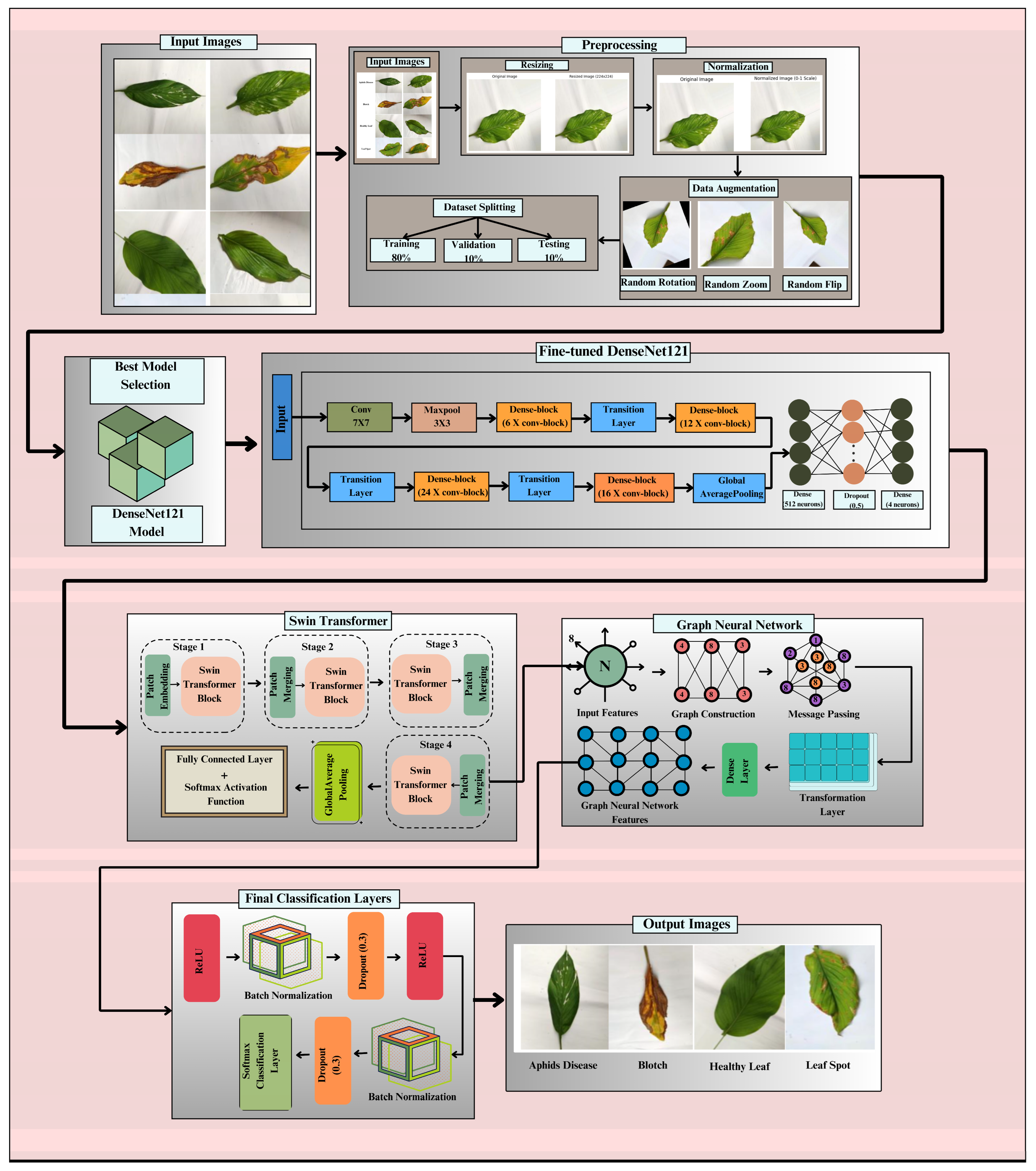
Figure 1: Proposed methodology for the classification of turmeric leaf disease.

3.1 Input Dataset

The dataset for this study was gathered from Mendeley, an open-source platform [20]. The dataset contains a total of four classes: Aphid Disease, Blotch, Healthy Leaf, and Leaf Spot. Fig. 2 demonstrates details about various leaf diseases in turmeric plants. It provides details of the disease, categorizing them based on disease presence and health status, including the name of the disease, cause, symptoms, and effects for every class.

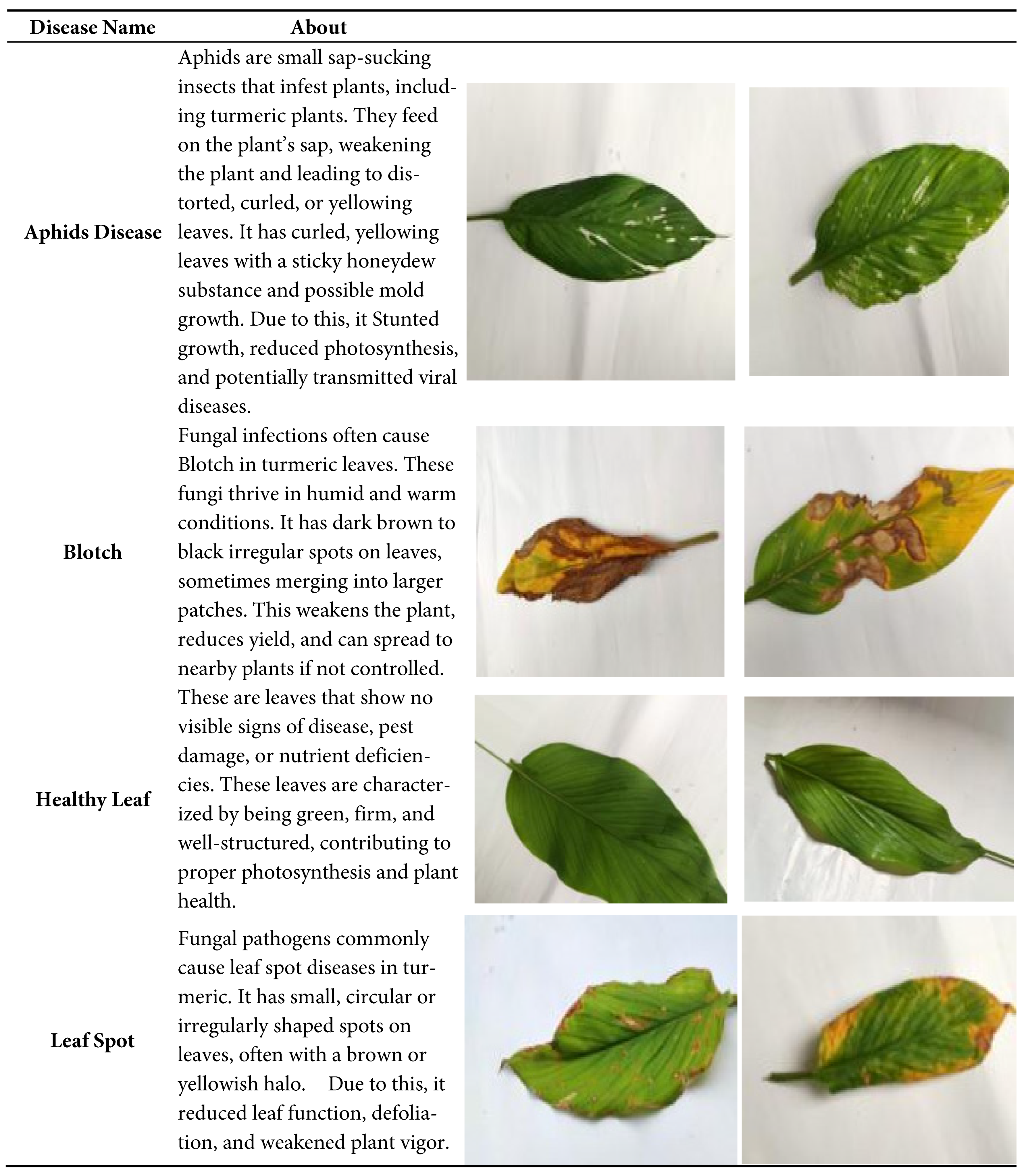
Figure 2: Input dataset.

The original dataset contains a total of 865 images and is further divided into four classes: Aphids Disease includes 221 images, Blotch contains 238 images, Healthy Leaf contains 213 images, and Leaf Spot contains 193 images. The distribution of images among classes of turmeric leaf disease is shown in Fig. 3.

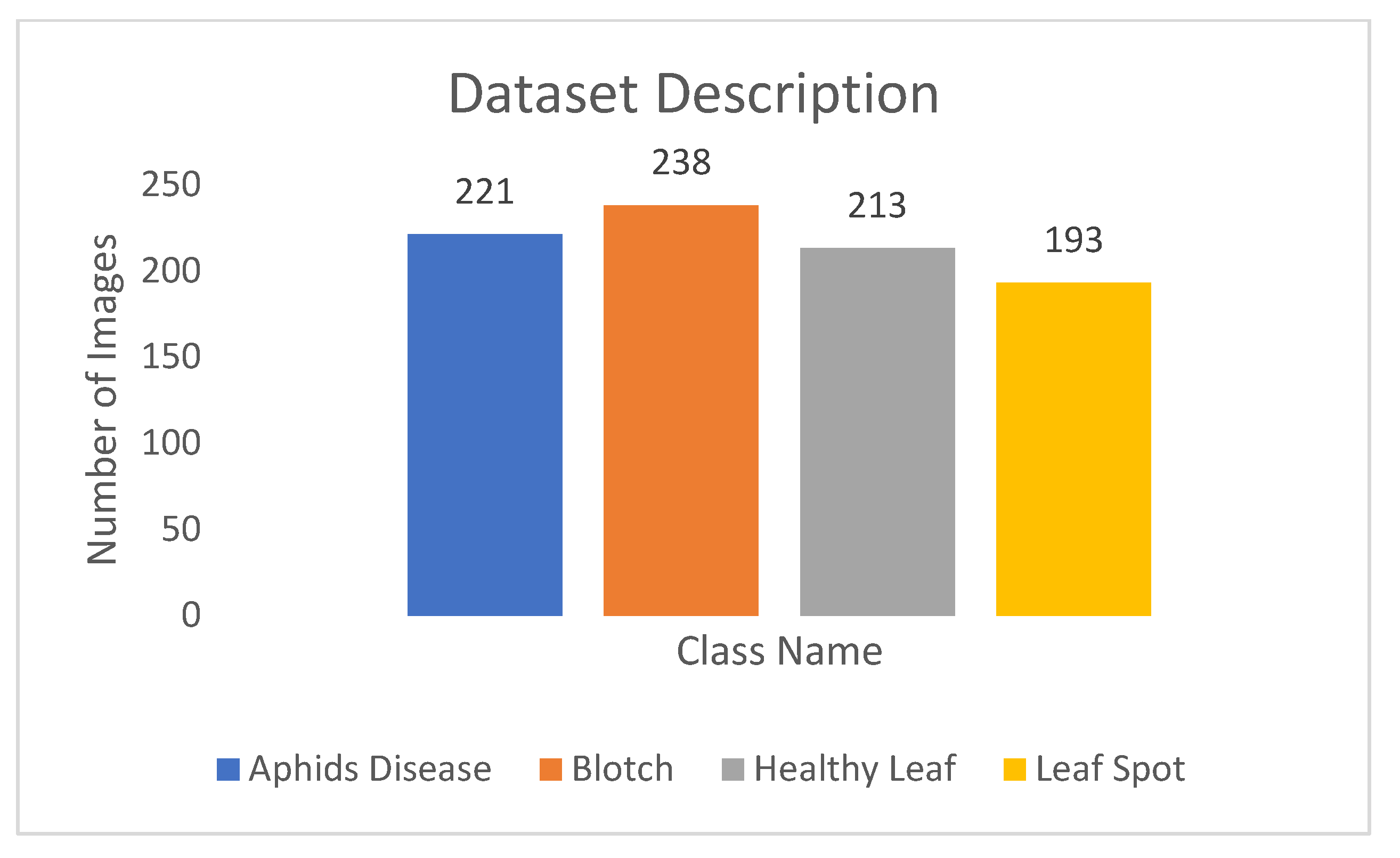
Figure 3: Distribution of images among classes of turmeric leaf disease.

3.2 Preprocessing

The preprocessing pipeline for turmeric leaf disease classification involves several crucial steps to ensure optimal model performance, as shown in Fig. 4. Initially, images are loaded from the dataset, which consists of four classes: Aphids Disease, Blotch, Leaf Spot, and Healthy Leaf.

After that, to maintain uniformity, images have been resized to 224 × 224 pixels, as the earlier images had different dimensions. I′=Resize(I,224,224)(1) where I is the original image and I′ is the resized image. Then, normalization is performed using per-image standardization, where each pixel value is normalized by subtracting the image mean and dividing by the image standard deviation, resulting in a zero mean and unit variance, as illustrated in Eq. (2). Normalization improves to promote convergence in training. Inorm=I−μσ(2) where I is the original image pixel values, μ is the mean pixel value of the image, and σ is the standard deviation of the image’s pixel values. After that, the dataset is split into three subsets: training, testing, and validation, with 80%, 10%, and 10%, respectively, ensuring an effective distribution for model evaluation as shown in Eqs. (3)–(5). The number of images in the training set is 693, and the number of images used for testing and validation is 86 each. Nval=validation_splitXN2=0.2XN2=0.1XN(3) LNtest=validation_splitXN2=0.2XN2=0.1XN(4) Ntest=validation_splitXN2=0.2XN2=0.1XN(5) where N is the total number of images in the dataset. For this study, N = 865, resulting in N t r a i n = 693, N v a l = 86 and N t e s t = 86. Then, data augmentation techniques are applied on training set, including random rotation as shown in Eq. (6), random zoom as shown in Eq. (7), random horizontal flipping as shown in Eq. (8), random brightness as shown in Eq. (9) and random translation as shown in Eq. (10) are employed to enhance dataset diversity and mitigate overfitting by artificially increasing the number of training samples. I′=Rotate(I,θ)(6) I′=Zoom(I,z)(7) I′=Flip(I,d)(8) I′=Brightness(I,β)(9) I′=Translate(I,tx,ty)(10) where θ is the rotation angle (in degrees), Z is the zoom factor, d is the flip direction, β refers to the brightness adjustment factor, and t x , t y are the horizontal and vertical translation offsets, respectively.

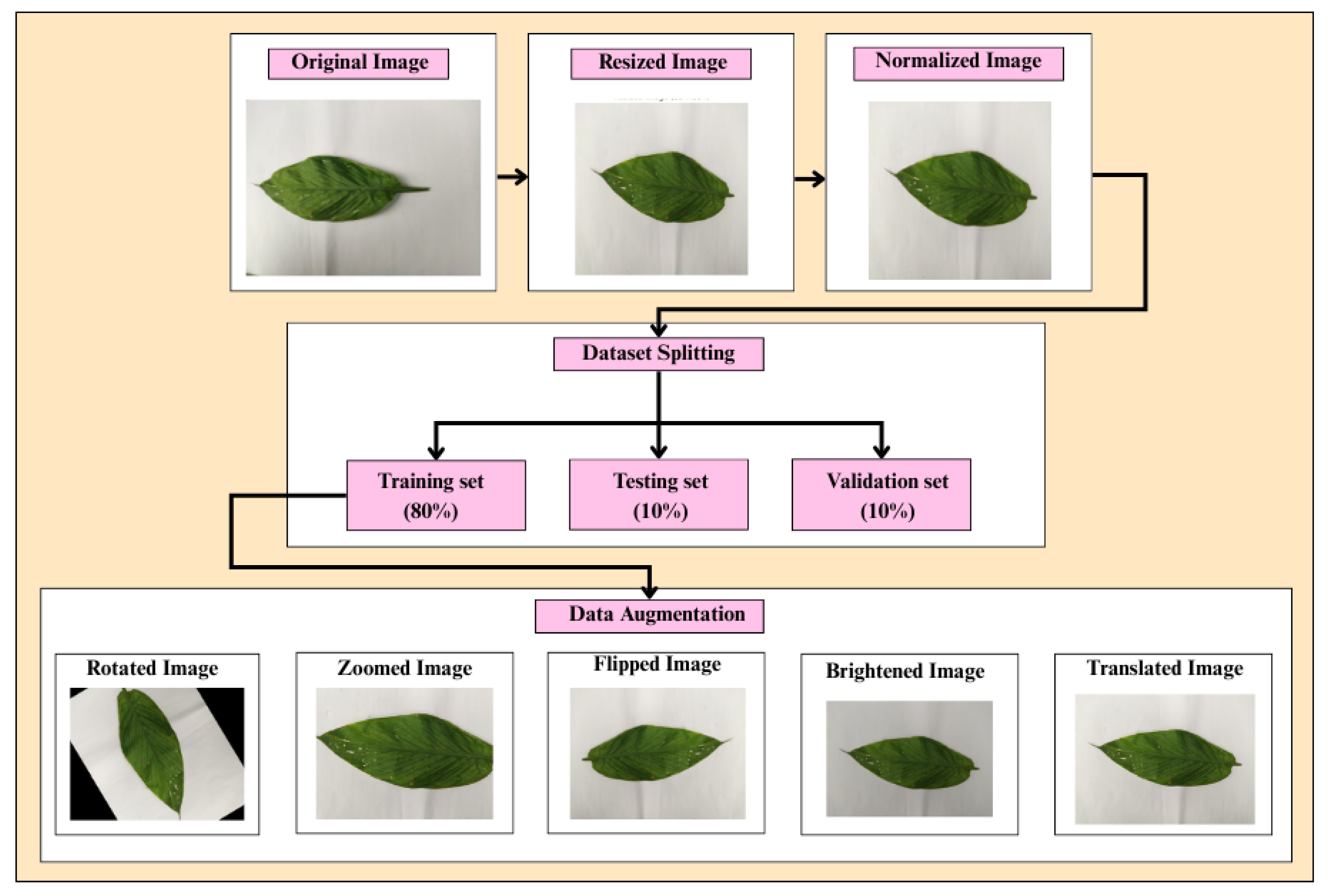
Figure 4: Flowchart for the preprocessing steps.

From a cybersecurity standpoint, the preprocessing pipeline and dataset handling are designed to ensure integrity and confidentiality of agricultural data. In real-world deployment, such systems can be enhanced with blockchain-based verification for dataset authenticity and access control mechanisms to prevent unauthorized modifications. Secure hash algorithms and cryptographically signed model checkpoints can further safeguard data and model integrity throughout the training lifecycle.

3.3 Selection of the Best Transfer Learning Model

DenseNet121 has been selected because it is an efficient model with good feature propagation and lower computation requirements compared to other deep models, as shown in Table 2. As opposed to regular deep networks, DenseNet121 incorporates dense connectivity where every layer gets feature maps from all the preceding layers. This architecture enhances the gradient flow, minimizes vanishing gradients, and facilitates feature reuse, improving performance with fewer parameters. DenseNet121 contains merely 8 million parameters, far fewer than VGG16 (138M) and ResNet50 (25.6M), yet it achieves comparable top-1 accuracy at 74.9%. Therefore, it is an excellent pick for computational cost without affecting the accuracy. Besides, its FLOPs (2.9 GFLOPs) are dramatically less than those of ResNet50 (4.1 GFLOPs) and InceptionV3 (5.7 GFLOPs), and therefore it can be deployed in actual applications, including edge and mobile devices.

Additionally, DenseNet121 is optimized for feature extraction in transfer learning, making it generalize effectively across various datasets with minimal training data. With these benefits, DenseNet121 is the best option for turmeric leaf disease classification, striking a balance between high accuracy, low parameter numbers, and computational efficiency over other deep learning models. Although Table 3 shows that EfficientNet-B0 achieves a slightly higher top-1 accuracy (77.1%) compared to DenseNet121 (74.9%) on the ImageNet benchmark, the choice of DenseNet121 as the primary backbone in this study was made based on practical performance, architectural compatibility, and feature connectivity considerations. EfficientNet-B0, despite being parameter-efficient, employs a compound scaling mechanism optimized for balanced depth, width, and resolution. However, it may underperform when fine-tuned on small, domain-specific datasets with limited image diversity, such as turmeric leaf images.

In contrast, DenseNet121’s dense connectivity pattern—where each layer receives feature maps from all preceding layers—enhances feature reuse, gradient flow, and stability during fine-tuning, which are crucial for medical and agricultural datasets characterized by subtle inter-class variations. Moreover, DenseNet121 integrates seamlessly with hierarchical and relational modules like the Swin Transformer and GNN, as it outputs a structured feature tensor (B, 1024, 7, 7) that can be readily reshaped into patch embeddings without extensive re-parameterization. Preliminary experiments also revealed that EfficientNet-B0, though computationally lightweight, produced less discriminative features for visually similar turmeric leaf classes, resulting in approximately 2–3% lower validation accuracy than DenseNet121 on the same dataset. Therefore, DenseNet121 was selected as the optimal trade-off between feature richness, stability, and integration flexibility, ensuring robust downstream performance in the proposed DenseSwinGNNNet architecture.

3.4 Proposed DenseSwinGNNNet Model

The proposed DenseSwinGNNNet architecture for classification of the turmeric leaf disease utilizes Swin Transformer and GNNs to improve feature learning and disease classification. The architecture shown in Fig. 5 is designed in a pipelined architecture, beginning with input images of turmeric leaves affected by various diseases. Preprocessing includes resizing, normalization, division of the dataset, and data augmentation, which are used to aid in the model’s generalization. The core of the model consists of two main components: Swin Transformer and GNN. The Swin Transformer begins with patch partitioning, whereby the input image is divided into patches of reduced size. These patches proceed through four hierarchical levels of Swin Transformer Blocks, which perform feature extraction based on self-attention while maintaining spatial relationships efficiently.

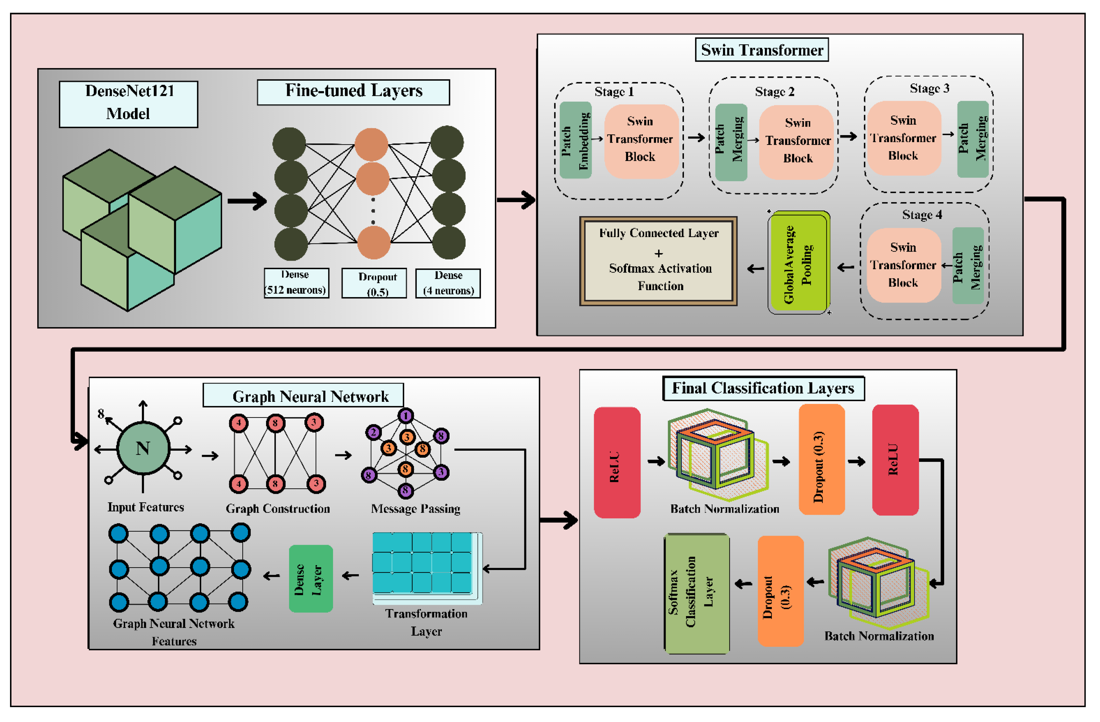
Figure 5: Architecture of proposed DenseSwinGNNNet.

Patch merging occurs in each of these steps to reduce resolution while enhancing feature representation. Global average pooling is carried out before feeding the extracted features to the classification network. GNN processes extracted deep features by building a graph representation of image features. The step of graph construction transforms the extracted features into nodes, with edges representing the connections between various regions of the image. The message-passing unit within the GNN updates feature embeddings by aggregating information from neighboring nodes, enabling the representation of intricate spatial and relational patterns in turmeric leaf diseases. A dense transformation layer further updates the feature representation before classification. The last classification layers utilize batch normalization, dropout (0.3 regularization), and ReLU activation functions to add learning stability. The output goes through a Softmax activation function that provides the probabilities for the four classes: Aphids Disease, Blotch, Leaf Spot, and Healthy Leaf. The output images indicate successful classification with varied forms of diseased and healthy leaves. By integrating Swin Transformer’s self-attention mechanism with the structured learning ability of Graph Neural Networks, DenseSwinGNNNet ensures highly discriminative feature learning, robust disease classification, and reduced misclassification risks. The dual approach enhances the accuracy and robustness of the model, achieving a promising deep learning solution for turmeric leaf disease diagnosis in precision farming.

3.4.1 Fine-Tuned DenseNet121 Model

The fine-tuned DenseNet121 model is based on a densely connected convolutional neural network architecture that seeks to maximize feature propagation and reuse. The model in Fig. 6 begins with a 7 × 7 convolution layer to extract low-level features, and then a 3 × 3 max-pooling layer to downsample the spatial dimensions while preserving essential patterns. The network consists of four Dense Blocks, each containing multiple convolutional layers (6, 12, 24, and 16 convolutional blocks, respectively). Each layer receives inputs from all the previous layers, promoting effective feature learning. Transition Layers between Dense Blocks are used to downsample using 1 × 1 convolutions and average pooling to achieve a balance between feature extraction and computational cost. After the final Dense Block, Global Average Pooling reduces the size of the feature map without sacrificing significant information. The fully connected layers consist of a dense layer of 512 units, a dropout layer (0.5 probability) to prevent overfitting, and a final dense layer of 4 units for the four turmeric leaf disease classes. It is fine-tuned to enhance classification accuracy using pretrained weights when fitted to the turmeric leaf disease dataset. The model balances computational complexity, feature reuse, and generalization well, making it highly suitable for image classification.

Figure 6: Architecture of fine-tuned DenseNet121.

3.4.2 Swin Transformer

Swin Transformer is a deep learning model that can process high-resolution images efficiently by capturing both local and global context information. In contrast to traditional Vision Transformers that perform self-attention on the whole image in quadratic computational complexity, the Swin Transformer introduces window-based attention for linear complexity while retaining strong feature extraction capacity. The architecture has a hierarchical pattern that increasingly fuses patches and improves representations, making it very effective for image classification problems, such as the detection of turmeric leaf disease.

The initial step in the Swin Transformer pipeline shown in Fig. 7 is patch partitioning, where the input image is divided into small, non-overlapping patches. Partitioning the image in this way allows the model to process it in a structured manner. The patches are embedded into a high-dimensional space by a linear embedding layer, transforming the raw pixel values into feature vectors that the transformer layers can process.

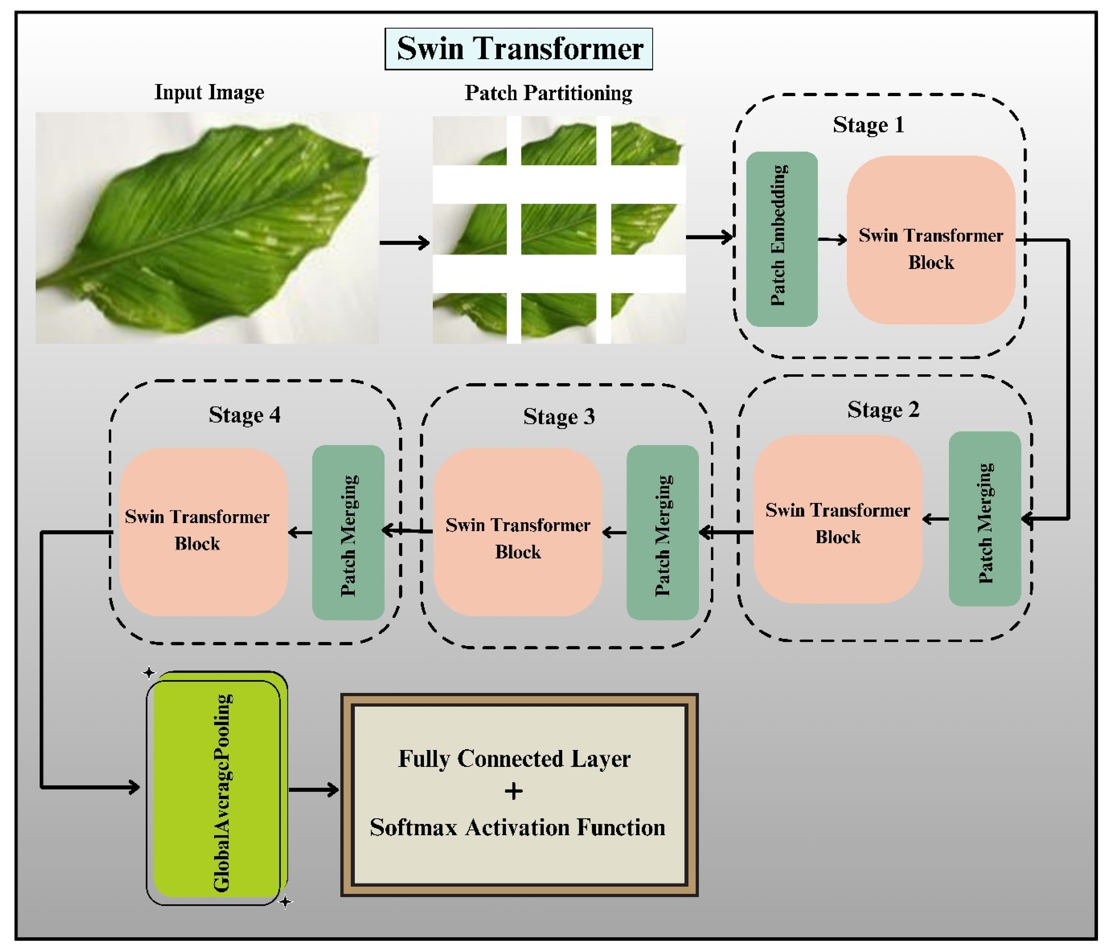
Figure 7: Architecture of swin transformer.

Mathematically, if an input image X of size H X W X C (height, width, and channels) is divided into patches of size P X P, the number of patches N is represented by Eq. (11):

Each patch is then projected into a feature space of dimension D, forming the initial feature representation in Eq. (12): Z0=f(X)(12) where f(.) represents the patch embedding function, instead of computing self-attention over the whole space, Swin Transformer adopts Window-Based Multi-Head Self-Attention (W-MSA). The process divides the feature map into non-overlapping windows and computes self-attention for each window separately, reducing computational complexity. The attention mechanism employs the regular scaled dot-product attention formula as presented in Eq. (13): AttentionQ,K,V=softmaxQKTdkV(13) where Q, K, V ∈ RMxd represent the query, key, and value matrices for each window of size M, and dk is the dimension of the key vector. The softmax operation ensures that the attention scores are normalized across all tokens within a window. To provide cross-window interaction without compromising computational efficiency, the Swin Transformer proposes shifted window attention. Between alternating layers, window partitioning is shifted by a constant offset, allowing information to propagate across adjacent regions. This technique is expressed in Eqs. (14) and (15): Z^l= W-MSALNZl−1+Zl−1(14) Zl=MLPLNz^l+Z^l(15) where W-MSA refers to windowed multi-head self-attention, LN is layer normalization and multi-layer perceptron (MLP) with a non-linear activation. These steps facilitate hierarchical learning of features, with lower layers learning fine-grained patterns and deeper ones learning more abstract representations.

The Swin Transformer operates on images in several stages, with each stage consisting of a Swin Transformer Block followed by patch merging. At every stage, the spatial resolution of the feature map decreases, while the feature dimension increases, much like how convolutional neural networks downsample images through pooling. The patch merging operation is mathematically defined in Eq. (16): Z′=Concat(Z1,Z2,Z3,Z4)Wp(16) where Z 1 , Z 2 , Z 3 , Z 4 are feature representations of neighbouring patches, and W p is a learnable weight matrix that projects the concatenated features into a new space. After hierarchical feature extraction, the final feature map undergoes global average pooling (GAP) to condense the information into a fixed-size vector, as shown in Eq. (17): ZGAP=1N∑i=1NZi(17) where N is the number of spatial locations in the feature map, as shown in Eq. (18). This vector is then transmitted through a fully connected layer and a softmax activation function for classification. y^=softmax(WZGAP+b)(18) where W and b are learnable parameters of the fully connected layer, and y ^ represents the predicted class probabilities. By integrating the Swin Transformer into the proposed model, it maximizes feature representation by extracting both fine-grained details and distant dependencies in images of turmeric leaf diseases. Its hierarchy of processing image data, while computationally efficient, makes the Swin Transformer a strong member in deep-learning models for classifying images.

3.4.3 Graphical Neural Network

A Graph Neural Network is a type of model in deep learning that has been designed specifically to manage and process graph-structured data. In contrast with usual neural networks used for Euclidean data, such as images and sequences, GNNs easily capture the relationships between objects in the form of nodes (vertices) and edges, formulating an organized framework. GNNs have found extensive applications in tasks like social network analysis, molecular property prediction, and medical diagnosis because they can represent very intricate dependencies among data points.

The structure of a GNN is of a systematic pipeline, as illustrated in Fig. 8. The core building blocks are feature extraction, graph construction, message passing, feature transformation, and dense classification layers. All of these are responsible for encoding and learning good representations from input features.

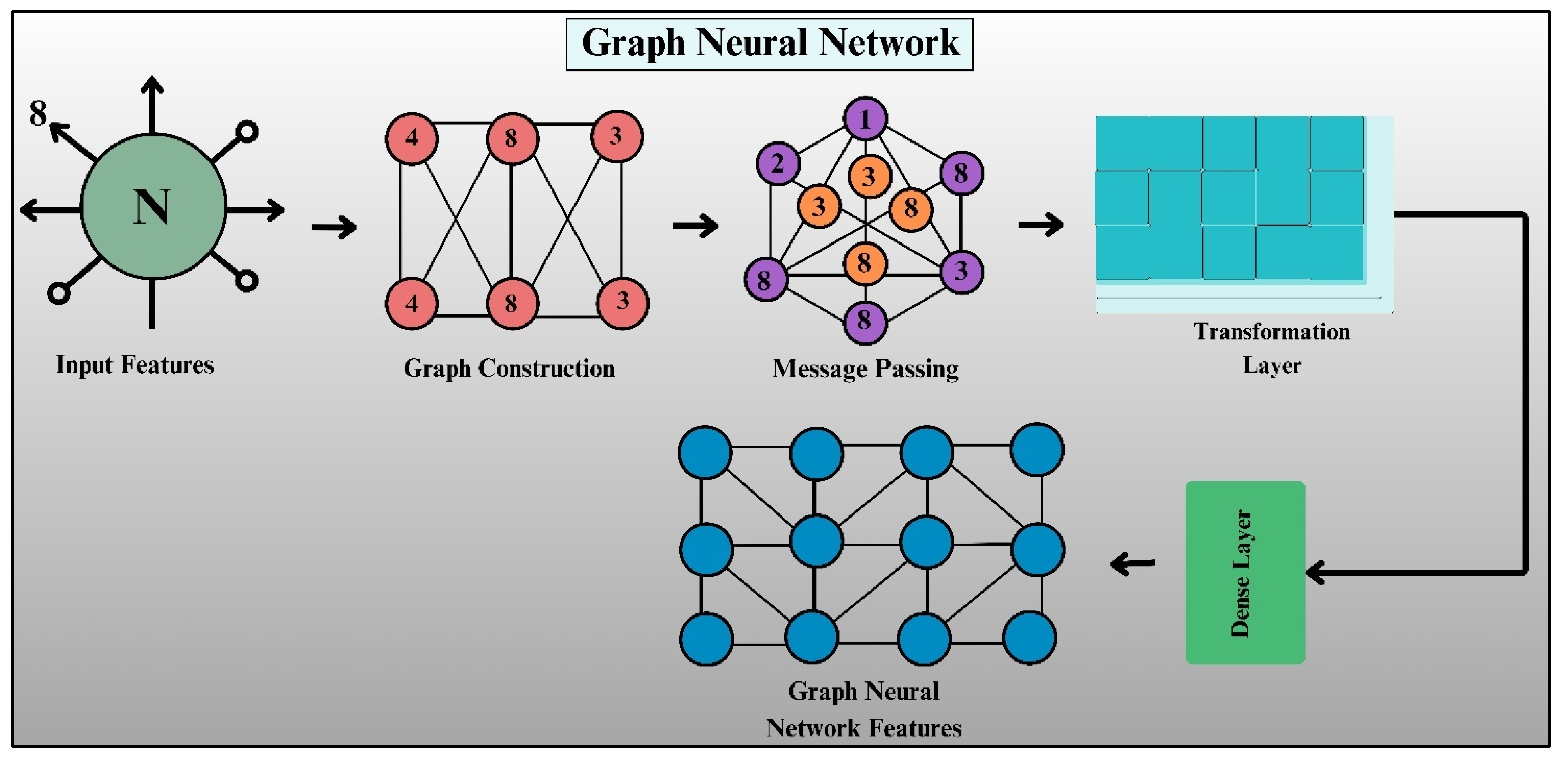
Figure 8: Architecture of graph neural network.

The initial process of GNN is extracting the input features of an entity (node). Every node comes with a feature vector that embraces its attributes. Let X denote the set of the input features, and each node v has a feature vector hv, denoted in Eq. (19): hv(0)=xv,v∈V(19) where h v ( 0 ) denotes the initial representation of the node, and V is the set of all nodes in the graph. These input features serve as the foundation for subsequent learning and representation updates. Once features are extracted, a graph is constructed by defining the connections (edges) between nodes. The relationships between nodes are represented using an adjacency matrix A, where each entry A i j Indicates the presence (or weight) of an edge between nodes i and j as shown in Eq. (20):

This adjacency matrix serves as the foundation for information propagation in the GNN. In weighted graphs, the values of A i j can be real numbers indicating the strength of connections. Message passing, in which a node repeatedly accumulates data from its neighbours to update its own representation, is the fundamental learning mechanism of GNNs. This is accomplished by combining transformation and neighbourhood aggregation. Eq. (21) is used to calculate a node v’s updated feature representation at layer l: hv(l)=σWl∑uϵNv1Nvhul−1+Blhvl−1(21) where h v ( l ) is the updated feature representation of node v at layer l, N(v) represents the neighbouring nodes of v, W l and B l are trainable weight matrices, σ is a non-linear activation function, h u l − 1 represents the feature vectors of neighbouring nodes from the previous layer. This equation ensures that each node receives information from its local neighbourhood, refining its feature representation iteratively. After multiple layers of message passing, each node learns a refined representation that captures its contextual relationships. The entire graph can be described using a feature matrix H ( l ) , which stacks all node representations at layer l. Using matrix notation, the feature update rule can be rewritten as shown in Eq. (22): H(l)=σA~Hl−1Wl(22) where, H ( l ) is the feature matrix of all nodes at layer l, A ~ is the normalized adjacency matrix ensuring stable training, W l is the learnable weight matrix. This formulation allows efficient propagation of node features throughout the graph, making GNNs highly effective in capturing relational structures. Once the GNN has processed the node features, a transformation layer is applied to restructure the learned representations into a more compact format. This transformation layer helps refine the output for improved classification.

Finally, the transformed features are passed through a dense layer, which performs the final classification based on the learned node representations. This step ensures that the extracted features are accurately mapped to their respective categories.

The incorporation of GNNs into the classification model addresses the disparity between global reasoning and local feature extraction. Unlike fully connected layers, which process feature dimensions individually, the GNN layer enables the explicit modeling of relationships between various components of features. This characteristic comes in handy for disease classification, where minute differences in texture, colour, and structure must be understood collectively. By utilizing the graph-based learning paradigm, the model effectively captures both contextual and spatial dependencies, resulting in stronger and more interpretable predictions.

In the proposed DenseSwinGNNNet architecture, the GNN module operates on feature embeddings derived from the Swin Transformer. After hierarchical attention processing, the final output feature map from the Swin Transformer, with dimensions [B, 16, 768], is used to construct a graph. In this graph, each patch embedding represents a node, and the spatial or contextual relationships among patches define the edges. The adjacency matrix A ∈ ℝn×n (where n = 16 nodes) is generated based on 8-connected spatial neighborhood criteria, meaning that each node is connected to its immediate surrounding patches. To enhance relational awareness, edge weights are computed using cosine similarity between patch feature vectors, ensuring that visually or semantically similar regions have stronger connections. This weighted adjacency matrix allows the GNN to aggregate features from both spatially and contextually relevant nodes during the message-passing process. The message-passing operation follows the standard update rule shown in Eq. (23): H(l+1)=σ(A¯H(l)W(l))(23) where H(l) denotes node embeddings at layer l, A ¯ is the normalized adjacency matrix, W(l) represents trainable weights, and σ is the ReLU activation. Two GNN layers were implemented, each followed by batch normalization and dropout (rate = 0.3) to improve stability and prevent overfitting. This design enables the GNN to effectively capture spatial correlations and inter-patch dependencies, enriching the learned feature space before final classification. The explicit graph construction, based on spatial proximity and feature similarity, not only ensures interpretability but also allows other researchers to replicate the framework using similar transformer-based feature embeddings.

3.4.4 Final Classification Layer

The final classification layer in the proposed model is significant for projecting the learned feature representations onto the actual class labels, as shown in Fig. 9. After the feature extraction and transformation processes, where the Swin Transformer and GNN blocks operate on the input data, the obtained features pass through a dense layer for the final classification. This is the last layer that sums up all the information obtained through extraction and then assigns probabilities to each class with a softmax activation. Mathematically, let X represent the feature vector output from the last GNN layer, where X ∈ R d is a d-dimensional feature representation. The classification layer applies a fully connected transformation, which is defined in Eq. (24): Z=WX+b(24) where W ∈ R C X d is the weight matrix, b ∈ R C is the bias term, and C represents the number of output classes. The transformed feature vector Z is then passed through a softmax activation function to obtain the final class probabilities as represented in Eq. (25): PyiX=eZi∑j=1CeZj(25) where P y i X represents the probability of class i, ensuring that all class probabilities sum to 1. By transforming the raw class scores into comprehensible probabilities, the softmax function enables the model to forecast the most probable class for the supplied input.

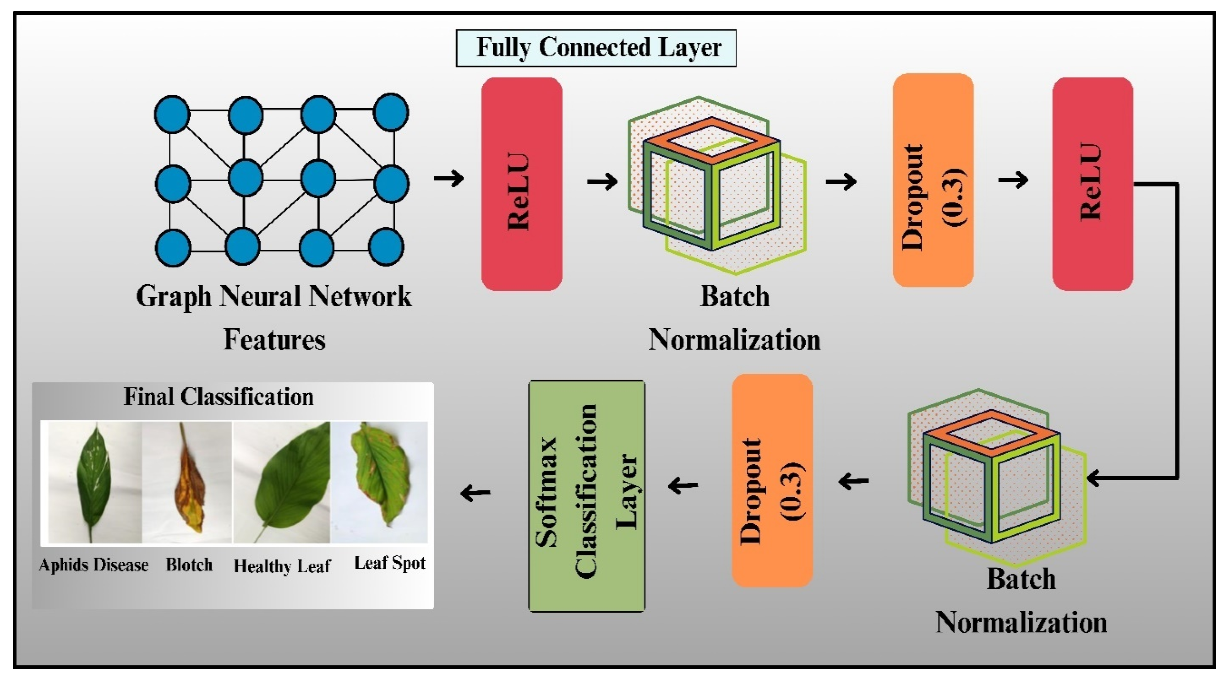
Figure 9: Architecture of final classification layers.

To improve the strength of the classification step, dropout regularization is applied before the final classification layer. Dropout randomly disables some neurons during training to prevent overfitting and ensure the model can generalize well to new, unseen data. The output from the dropout layer is then fed to batch normalization, which normalizes the activations and makes the training stable.

The whole process of classification is optimized with the sparse categorical cross-entropy loss function, as shown in Eqs. (26) and 27: H(l)=σA~Hl−1Wl(26) L=−∑i=1CyilogP(yi|X)(27) where y i represents the actual class label in one-hot representation. This loss function computes the difference between the predicted probabilities and true labels, helping the optimization process reduce classification errors. Optimization is carried out using an adaptive learning rate optimizer like AdamW, which adapts the weight updates during run-time to improve convergence rates and model performance.

4 Results

The result section provides a descriptive analysis of the constructed DenseSwinGNNNet model for turmeric leaf disease classification. The section begins with a descriptive performance analysis, comparing the proposed model with the best model selection architectures: DenseNet121 and DenseNet121 with Swin Transformer. Various performance parameters, such as accuracy, precision, recall, and F1-score, are analyzed to measure the strength of classification. An optimizer analysis is also discussed to determine the best optimization technique. To make model evaluation transparent, it is highlighted that all final quantitative outcomes reported in this section, such as the accuracy, precision, recall, F1-score, and Area Under the Curve (AUC) values calculated in the analysis based on the classification parameters table and the visual analyses through the confusion matrix displayed in figures, were extracted solely from the held-out 10% test set. This part of the dataset was completely unseen during the training and validation processes and was reserved solely for the final evaluation. This separation ensures that the reported performance metrics reflect the actual generalization capability of the suggested DenseSwinGNNNet model on unseen data, with no overlap or information leakage between the training, validation, and testing phases.

4.1 Experimental Setup

The envisioned DenseSwinGNNNet model was deployed using the PyTorch deep learning framework (version 1.13.1) with CUDA 11.6 for GPU acceleration. Model training was run with a batch size of 32, which gave an adequate trade-off between memory usage and gradient stability. Training was done for 30 epochs, a configuration established empirically to achieve convergence without overfitting. The Adam optimizer was implemented for its adaptive learning rate adjustment and convergence speed properties, with the initial learning rate set at 0.001. The use of this optimizer, coupled with the comparably small learning rate, facilitated smooth updating throughout training for all the network elements. Every training epoch took around 30 s on the utilized hardware setup, making the overall training time almost 1.25 h.

Regarding model complexity, DenseSwinGNNNet contains around 25.3 million trainable parameters, indicating the depth and capability of the combined architecture involving DenseNet, Swin Transformer, and Graph Neural Network elements. While possessing significant representational capability, the computational expense of the framework under consideration remains low, with each forward pass making 5.8 GFLOPs of computations. These computational features demonstrate that the framework under consideration has achieved a trade-off between efficiency and accuracy, supporting deployment in research and real-world agricultural monitoring applications. The specific configuration settings are reported, by presenting a clear overview of the experimental setup to ensure reproducibility and enable comparison with current methods documented in the literature.

4.2 Result Analysis of DenseNet121 Model

The training and validation plots of the DenseNet121 model used for classifying turmeric leaf disease, shown in Fig. 10, offer insight into how the model learns during training. Training is conducted with the Adagrad optimizer over 30 epochs, using a learning rate parameter of 0.0001 to ensure adaptive learning rate adjustment for convergence stability. The training and validation accuracy plot in Fig. 10a shows a steady increase in training accuracy over 0.95, while validation accuracy remains constant at around 0.85. This indicates that the model learns quickly but experiences minimal overfitting, as evidenced by the increasing gap between the training and validation curves. The graph of training and validation loss in Fig. 10b reveals a general drop in both losses. The training loss plummets at the start and then levels off, while the validation loss drops slightly before leveling off, supporting the mild overfitting. The precision graph in Fig. 10c reveals that training precision approaches 0.99, while validation precision levels off at approximately 0.90, reflecting high positive class detection but small misclassifications. The recall plots in Fig. 10d show that training recall increases towards 98%, while validation recall oscillates between 0.85 and 0.90. This suggests the model picks up most diseased and healthy leaves but has some trouble with false negatives. The F1-score plot in Fig. 10e follows recall and precision patterns, with training F1-scores approaching 98%, whereas validation F1-scores increase before leveling off just below 90%, indicating a balance between precision and recall.

Figure 10: Graphical analysis of DenseNet121 model based on training and validation, (a) Accuracy, (b) Loss, (c) Precision, (d) Recall, and (e) F1-score.

The confusion matrix in Fig. 11 illustrates the DenseNet121 model’s classification performance in separating four tea leaf categories: Aphids Disease, Blotch, Healthy Leaf, and Leaf Spot. The diagonal elements are correctly classified samples, whereas the off-diagonal elements are the misclassifications. The model has good discriminative power, correctly classifying 21 out of 22 Aphid Disease samples, 22 out of 24 Blotch samples, 15 out of 19 Healthy Leaf samples, and 20 out of 21 Leaf Spot samples. There are some misclassifications, notably one Aphid Disease image classified as Healthy Leaf and three Healthy Leaf samples predicted to be Leaf Spot, suggesting a visual similarity between the two classes. Overall, the DenseNet121 model has a high accuracy rate, effectively capturing complex visual patterns and textural changes in both diseased and healthy leaf specimens. The slight differences show possible visual feature overlap, which could be further reduced by using high-level feature enhancement or attention mechanisms. This robust confusion matrix result demonstrates the model’s aptitude for automated disease diagnosis in precision agriculture and presents an effective and reliable method for early detection and classification of tea leaf diseases.

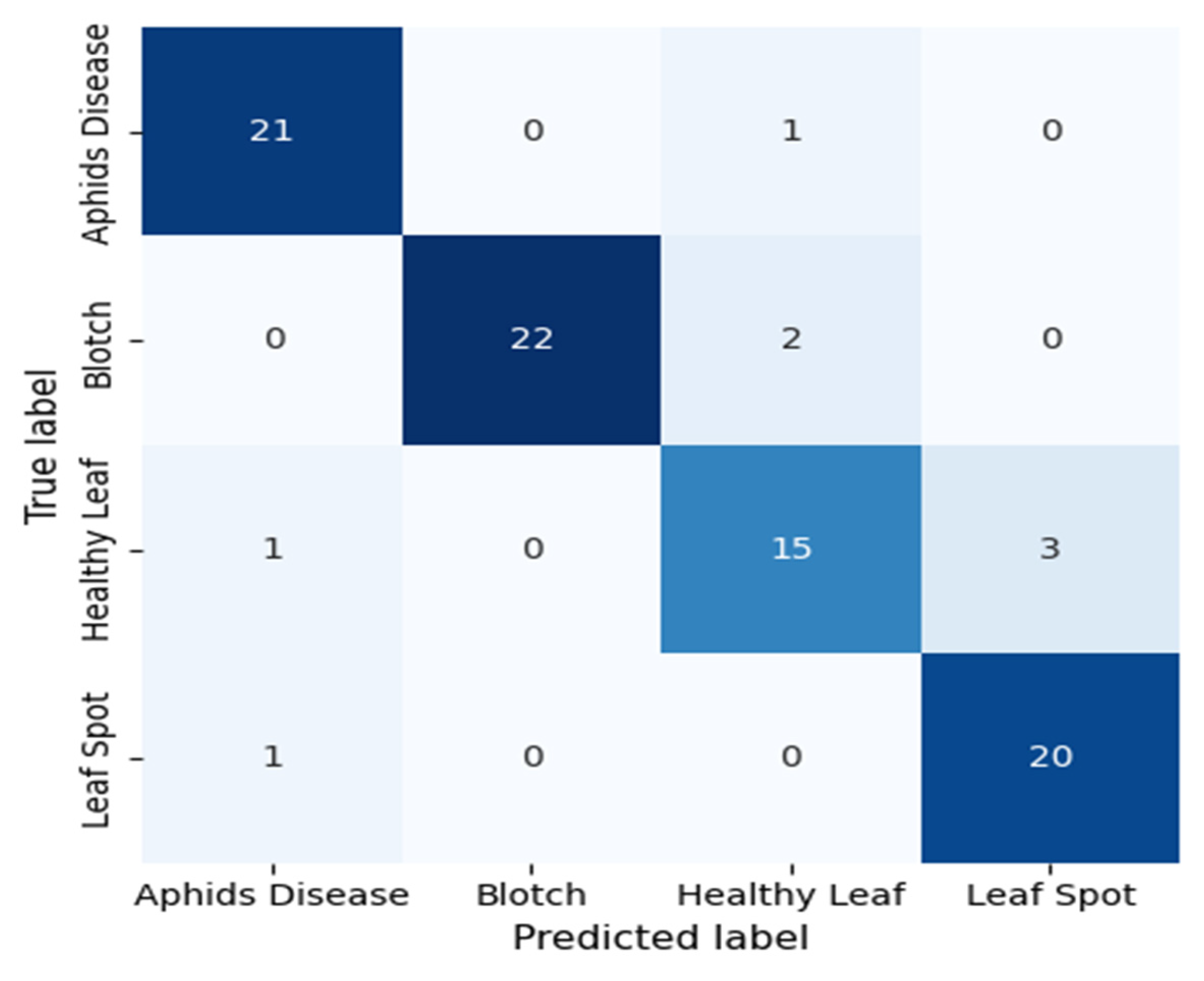
Figure 11: Confusion matrix of the proposed DenseNet121 model evaluated on the held-out 10% test set, illustrating correct and misclassified samples for the four turmeric leaf disease classes.

The performance of the model depicted in Table 4 clearly illustrates its high proficiency in correctly classifying different tea leaf conditions. It resulted in a precision of 0.91, a recall of 0.95, and an F1-score of 0.93 for Aphids Disease, which reflects a very dependable performance with fewer false predictions. For the Blotch class, the model achieved maximum precision (1.00) with a recall of 0.91, indicating that all instances of Blotch predicted were accurate, but a negligible number of actual cases were omitted. The Healthy Leaf class exhibited relatively lower values (precision 0.83, recall 0.78, F1-score 0.81), indicating moderate complexity in distinguishing healthy from diseased ones due to minute textural and color similarities. Conversely, Leaf Spot has a well-balanced performance with a recall of 0.87 and a precision of 0.95, which is indicative of the model’s effectiveness in recognizing this type of disease. Generally, the DenseNet121 model demonstrates strong classification power across all classes, achieving very high accuracy in recognizing diseased leaves. The slightly lower scores on the Healthy Leaf class represent an area of potential improvement, likely due to increased feature extraction or fine-tuning of class-specific features. These findings confirm the model’s applicability to real-world use in automated plant disease detection systems.

The ROC curve for the classification of turmeric leaf diseases with DenseNet121, as shown in Fig. 12, illustrates the model’s diagnostic power for four classes. The AUC values represent the performance of the classifier. The Healthy Leaf class achieved the highest AUC of 0.96, demonstrating an excellent balance between sensitivity and specificity. The model is capable of differentiating healthy leaves from diseased leaves. The Blotch class was next with an AUC of 0.94, indicating a very high true positive rate and very low false positives, further assuring the reliability of the model in identifying Blotch-infected leaves. The Leaf Spot class resulted in an AUC of 0.89, indicating good classification performance but with relatively higher false positive rates compared to Blotch and Healthy Leaf. The Aphids Disease class achieved an AUC of 0.88, indicating the model’s decent discriminative capability between Aphids Disease and other classes. However, there is potential for improvement, possibly due to the visual resemblance between Aphid Disease and other leaf diseases. The DenseNet121 model consistently demonstrates high discriminative capability, as all AUC values are greater than 0.85, highlighting its strong performance in classifying turmeric leaf diseases. The ROC curves also show a significant gap between the Healthy Leaf class and the rest, reflecting the model’s improved ability to identify healthy samples, which is essential for reducing false alarms in actual agricultural environments. The slightly lower AUC for Aphids Disease suggests the need for additional feature extraction layers or hyperparameter fine-tuning to enhance classification accuracy.

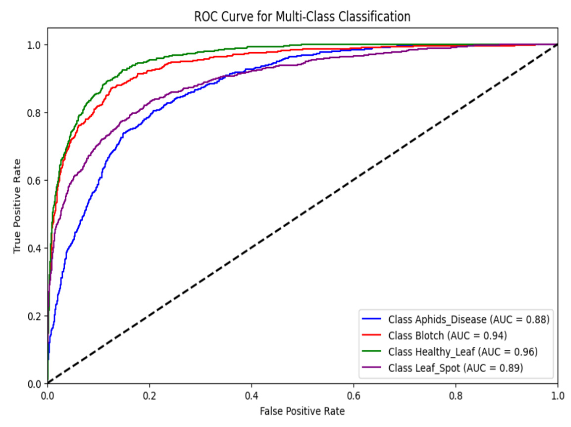
Figure 12: Analysis of DenseNet121 model based on ROC curve.

4.3 Result Analysis of DenseNet121 with Swin Transformer

The performance of the DenseNet121 model with Swin Transformer for turmeric leaf disease classification is evaluated using different training and validation metrics, as shown in Fig. 13. The model is optimized with the Adagrad optimizer using 30 epochs and a learning rate of 0.0001, enabling adaptive learning rate adjustment to enhance convergence. The accuracy plots of Fig. 13a reveal a smooth rise, with the training and validation accuracy curves converging after about 10 epochs. This reflects successful learning with little overfitting, as the validation curve closely matches the training curve. The loss plots in Fig. 13b reflect a descent trend, with the validation loss leveling off after about 15 epochs. Small fluctuations in validation loss indicate minor overfitting, which can be countered using regularization methods. The graphs of precision in Fig. 13c show a consistent increase, with the validation precision stabilizing after 10 epochs, indicating excellent generalization capability. The recall plots in Fig. 13d also follow the same trend, showing optimal performance within the first 10 epochs, which indicates that the model can detect diseased leaves with minimal false negatives. Finally, the graphs of F1-scores in Fig. 13e, a balance between precision and recall, indicate a pattern of stabilization beyond 10 epochs, affirming the model’s stability. A slight fluctuation in validation loss and accuracy supports the need for a bit more fine-tuning to improve classification further. All these results establish the efficacy of the DenseNet121 with the Swin Transformer method for the accurate classification of turmeric leaf diseases.

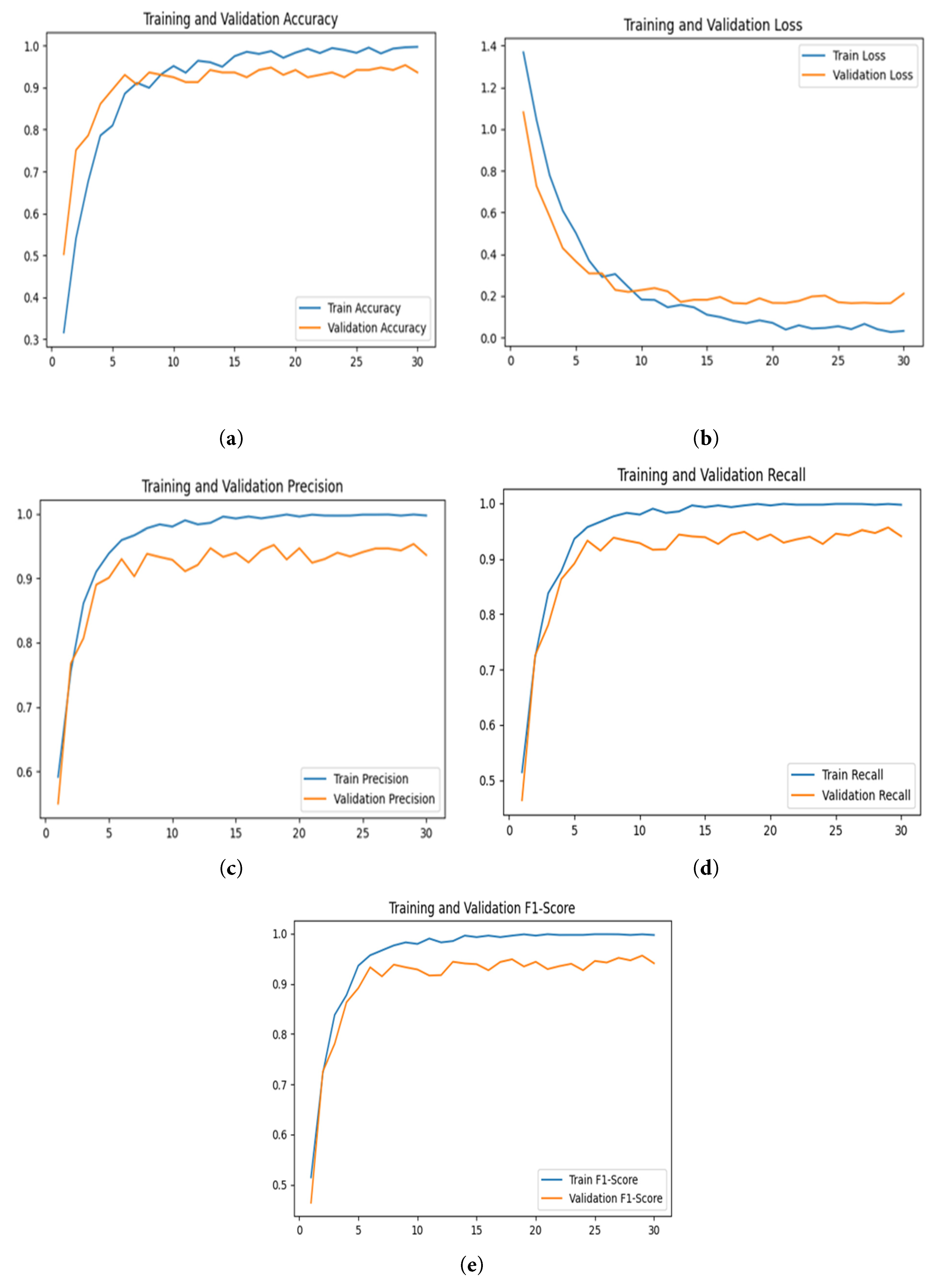
Figure 13: Graphical Analysis of DenseNet121 and Swin Transformer model based on Training and Validation (a) Accuracy, (b) Loss, (c) Precision, (d) Recall, and (e) F1-Score.

The confusion matrix shown in Fig. 14 indicates the relative classification performance of the DenseNet121 and Swin Transformer models on four tea leaf classes: Aphids Disease, Blotch, Healthy Leaf, and Leaf Spot. The two models are both excellent discriminators, achieving very high true positive rates across all classes and few misclassifications. For Aphids Disease, 21 out of 22 were well classified, one was misclassified as Leaf Spot, indicating the high sensitivity and robustness of the model. For Blotch, most samples (21 out of 24) were accurately predicted, with little confusion between Aphids Disease and Healthy Leaf, indicating minor overlaps in visual texture. The Healthy Leaf class had almost flawless classification, with all 19 correctly classified, highlighting the models’ sensitivity to the differentiation between healthy and diseased patterns. For Leaf Spot, 20 of the 21 instances were correctly identified, further confirming the models’ accuracy. Overall, the confusion matrix shows both DenseNet121 and Swin Transformer accurately capturing complex spatial and colour characteristics. Yet, the Swin Transformer achieves a slight improvement in coping with inter-class similarities as a result of its self-attention mechanism, whereas DenseNet121 provides effective feature reuse with dense connections. Overall, these findings highlight the high accuracy, generalizability, and robustness of both models in plant disease classification.

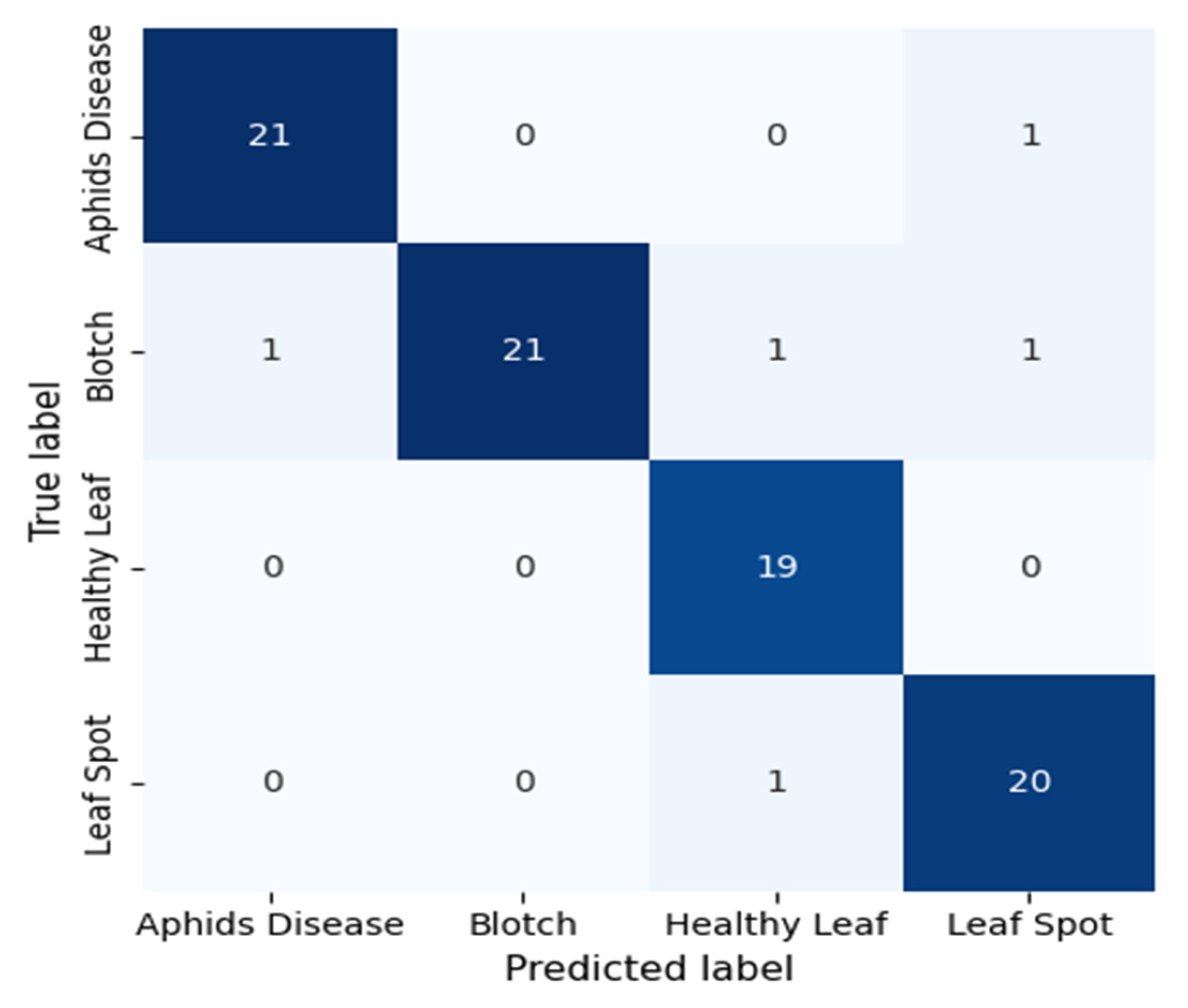
Figure 14: Confusion matrix of the proposed DenseNet121 and Swin transformer model evaluated on the held-out 10% test set, illustrating correct and misclassified samples for the four turmeric leaf disease classes.

The analysis of the DenseNet121 and Swin Transformer models’ performance, based on the classification metrics presented in Table 5, emphasizes their robust and reliable ability to classify various tea leaf conditions with high precision and consistency. For Aphids Disease, both models achieved a balanced precision and recall of 0.95, resulting in an F1-score of 0.95, which reflects highly accurate and consistent predictions with zero false negatives or positives. The Blotch class achieved complete precision (1.00) and a recall of 0.87, indicating that all Blotch predictions were correct. However, some true cases were not identified, possibly due to their visual resemblance to other infected leaves. The Healthy Leaf class also performed remarkably well, achieving a precision of 0.90, a recall of 1.00, and an F1-score of 0.95, indicating the models’ capacity to identify healthy samples correctly with zero misclassification. For Leaf Spot, the models demonstrated a strong balance with 0.90 precision and 0.95 recall, indicating strong detection ability. In total, DenseNet121 and Swin Transformer both performed well across all classes, with the Swin Transformer performing slightly better than DenseNet121 because of its self-attention mechanism that further improves global feature comprehension. The metrics as a whole confirm the robustness, generalization capability, and applicability of the models for effective automated plant disease diagnosis.

ROC curve of the fine-tuned model for the classification of turmeric leaf disease from Fig. 15 clearly indicates the discriminative ability of the model for all four classes, i.e., Aphids Disease, Blotch, Healthy Leaf, and Leaf Spot. AUC values of each class indicate the model’s capability to discriminate between positive and negative examples. Aphid disease had an AUC of 0.88 with excellent discrimination between true positives and negatives. Blotch had an AUC of 0.85, indicating the relatively high precision of the model, but with slightly more feature space overlap than Aphids Disease. The AUC was adjusted to 0.89 for Healthy Leaf, indicating the model’s good ability to differentiate healthy from diseased leaves, a very crucial feature in precision agriculture. Leaf Spot had an AUC of 0.82, the lowest of all classes, indicating a moderate level of confusion with other diseases due to the possible visual similarity of leaf patterns. ROC curves for all classes climb well above the diagonal random guess line, which signifies that the model is significantly better than random probability. The steep initial bends for Aphids Disease and Healthy Leaf reflect high sensitivity at low false positive rates, which is a good property for reducing misclassification in practice. The comparatively less flat leaf spot bend shows potential for improvement, possibly with more data or additional fine-tuning.

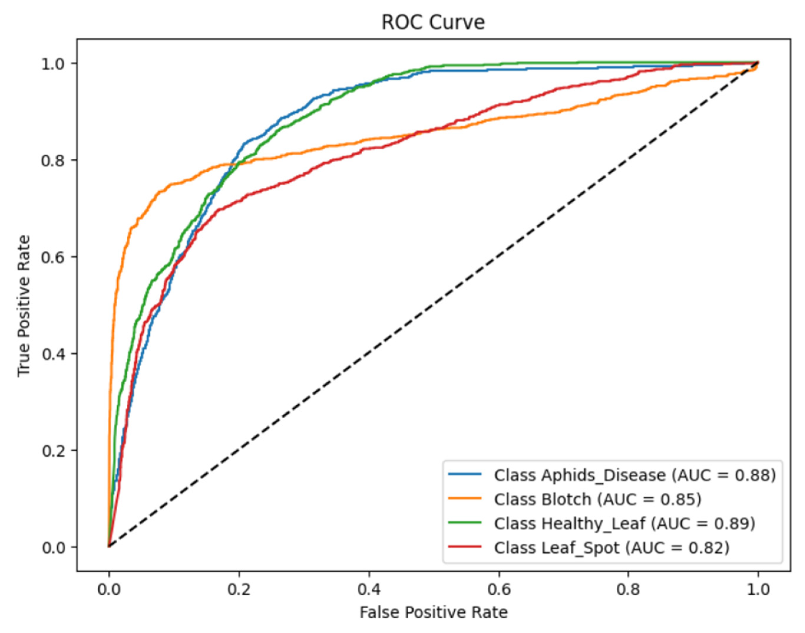
Figure 15: Analysis of DenseNet121 and Swin transformer model based on the ROC curve.

4.4 Result Analysis of Proposed DenseSwinGNNNet Model (DenseNet121, Swin Transformer, and Graph Neural Network)

The training and validation performance metrics of the proposed model for turmeric leaf disease classification are graphically represented in Fig. 16, with results plotted over 30 epochs. The model is trained with the Adagrad optimizer with a learning rate of 0.0001, with adaptive learning rate adjustment for stable convergence. The Training and Validation Accuracy graph in Fig. 16a illustrates steadily improving accuracy curves for both sets. These curves initially rise steeply during the earlier epochs before gradually leveling off, eventually converging to 0.90, which marks the strong learning and generalizing capabilities of the model. The plot of Training and Validation Loss in Fig. 16b shows a continuous decline in both losses, with the validation loss remaining slightly less than the training loss, indicating that the model is learning effectively without notable overfitting. The Training and Validation Precision plot in Fig. 16c shows a steep rise in early epochs, with both precision values exceeding 95%, demonstrating the model’s ability to identify positive cases and reduce false positives accurately. Likewise, the Training and Validation Recall plot in Fig. 16d is similar, with recall values above 0.90, affirming the model’s high sensitivity in identifying diseased and healthy leaves correctly. The Training and Validation F1-Score graph in Fig. 16e shows a gradual increase in both values, reaching close to 0.95, indicating well-balanced performance between recall and precision. The proximity of the training and validation curves for all the metrics also ensures that the proposed model exhibits stable generalization, rendering it highly efficient in classifying turmeric leaf disease.

Figure 16: Graphical analysis of proposed DenseSwinGNNNet model based on training and validation. (a) Accuracy, (b) Loss, (c) Precision, (d) Recall, and (e) F1-score.

The confusion matrix in Fig. 17 shows the classification accuracy of the presented DenseSwinGNNNet model on four tea leaf classes: Aphids Disease, Blotch, Healthy Leaf, and Leaf Spot. The model demonstrates outstanding accuracy and robustness, performing near-perfect classification on all classes with very few misclassifications. In particular, 21 out of 22 samples for Aphids Disease were accurately classified, while one was mistakenly classified as Leaf Spot, reflecting high discriminative ability and sensitivity. Similarly, the Blotch class exhibits excellent performance, correctly predicting 23 out of 24 cases, with only one slight confusion in the case of Aphids Disease. The Healthy Leaf class exhibited perfect classification, with all 18 samples correctly identified, indicating the model’s high ability to distinguish healthy leaves from infected ones. The Leaf Spot class also performed perfectly, with all 21 cases being properly identified, indicating the model’s strength in recognizing disease-pattern-specific features.

On the whole, the DenseSwinGNNNet model exhibits excellent feature learning by incorporating DenseNet’s hierarchical feature reuse, Swin Transformer’s global attention mechanism, and GNN’s relational reasoning. This synergy of combined strengths facilitates effective spatial-contextual awareness with minimum inter-class confusion. The confusion matrix verifies that DenseSwinGNNNet exhibits excellent generalization and robustness, rendering it highly effective for precision-based leaf disease detection and agricultural automation.

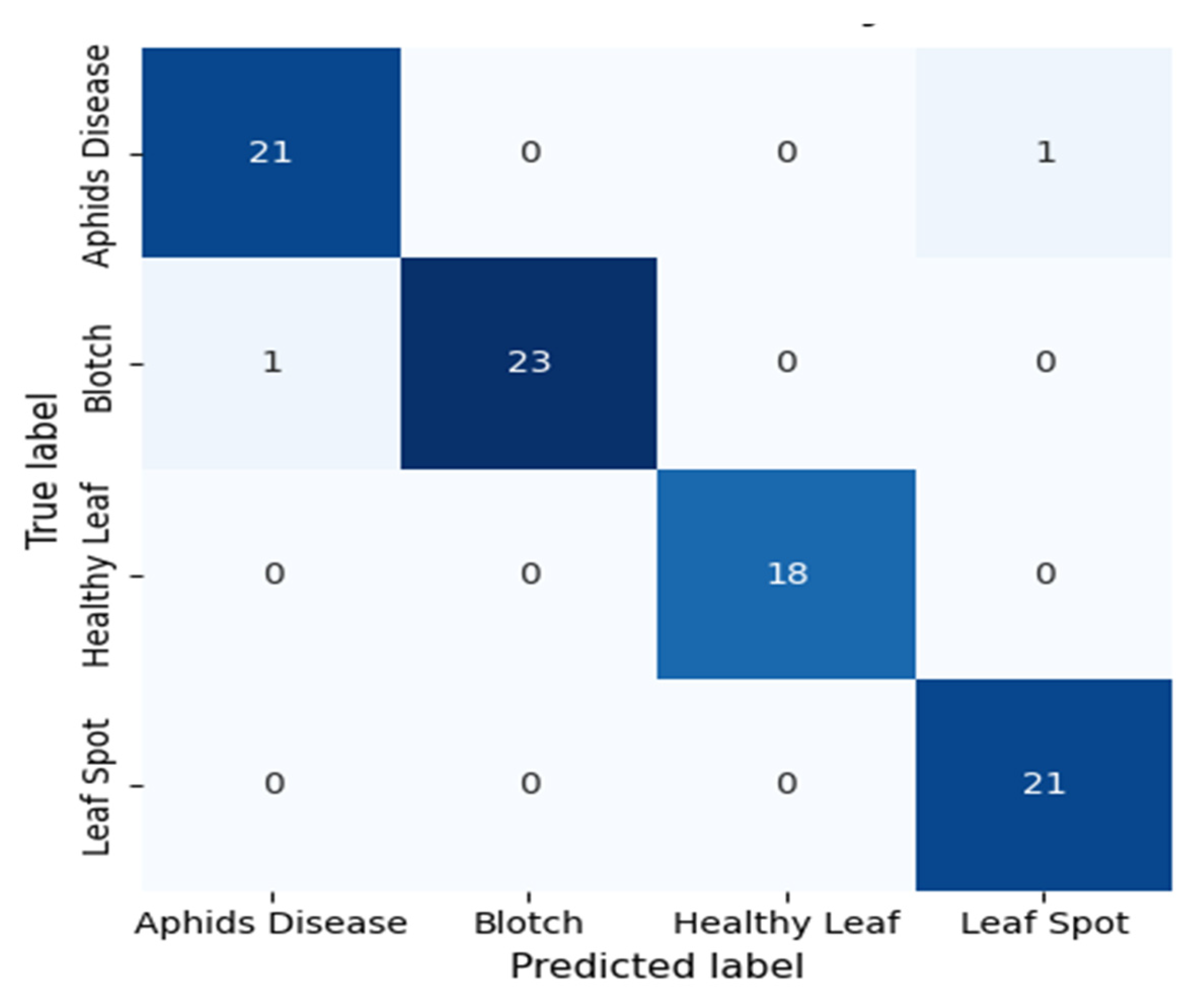
Figure 17: Confusion matrix of the DenseSwinGNNNet model evaluated on the held-out 10% test set, illustrating correct and misclassified samples for the four turmeric leaf disease classes.

The classification performance assessment of the developed DenseSwinGNNNet model, as shown in Table 6, confirms its exemplary capability to effectively detect and classify tea leaf diseases with great precision, recall, and F1-scores for all classes. For the Aphids Disease class, the model has a well-balanced precision, recall, and F1-score of 95% which indicates its high predictive dependability and low misclassifications. The Blotch class achieved perfect accuracy (100%) and a recall of 95%, with an F1-score of 97%. This means that all the predicted instances were correct, and a few actual samples were left behind. Notably, the Healthy Leaf class achieved perfect accuracy (100% precision, recall, and F1-score), validating the model’s ability to identify healthy leaves as opposed to the diseased ones with unqualified accuracy. Likewise, the Leaf Spot class exhibited an accuracy of 95% and a recall of 100%, providing an F1-score of 97%. This highlights the model’s strength in identifying and accurately classifying even fine disease symptoms. These regular and high values on all evaluation metrics confirm that DenseSwinGNNNet convincingly integrates dense connectivity, self-attention models, and graph-based spatial reasoning to obtain superior feature representation and contextual understanding. Therefore, the model exhibits outstanding generalization, stability, and reliability, making it very apt for practical agricultural disease detection use cases.

The ROC curve of the suggested model for classifying turmeric leaf disease is presented in Fig. 18, illustrating the model’s discriminative power among the four classes. AUC values represent the capacity of the model to distinguish among classes, with Aphids Disease at 0.97, Blotch at 0.98, Healthy Leaf at 0.99, and Leaf Spot at 0.97. These close to 1.0 AUC values for all these indicate that the model has an exceptionally good sensitivity (true positive rate) and specificity trade-off, making it least likely to misclassify. The Healthy Leaf class shows the best AUC, which means the model effectively discriminates the healthy from the pathological samples. Aphid disease and Leaf Spot classes with AUCs of 0.97 are representative of the model’s ability to classify these diseases with minimal misclassification. The Blotch class also displays a high AUC of 0.98, once more representing the model’s power. The sharp rise of the curves towards the top-left corner of the plot confirms that the model achieves high true positive rates even at low false positive rates. The slight variations between the curves indicate some degree of class overlap, possibly due to the visual resemblance between diseased and healthy leaves. However, the high AUC values confirm that the model performs these tasks exceptionally well.

Figure 18: Analysis of proposed DenseSwinGNNNet model based on ROC curve.

4.5 Optimizer Analysis for Proposed DenseSwinGNNNet Model

Optimizer analysis of the suggested DenseSwinGNNNet model compares the effects of various optimization algorithms—Adagrad, RMSprop, and Adam—on classification accuracy, based on average precision, recall, F1-score, and accuracy, as shown in Table 7. Adagrad optimizer provides 95.2% precision, 95.5% recall, and 95.7% F1-score with a general accuracy of 94%, reflecting effective learning but comparatively lower generalization than other optimizers. The RMSprop optimizer significantly enhances performance, achieving 98.5% precision, 98.2% recall, 98.7% F1-score, and 98% accuracy, reflecting greater optimization and training stability. Nonetheless, the Adam optimizer performs the best among them, achieving 99.5% accuracy across all measurements and an average accuracy of 98.71%, reflecting its excellence in tackling the complex feature distributions of turmeric leaf disease classification. The consistent improvement in performance from Adagrad to RMSprop and subsequently to Adam indicates that adaptive learning rate techniques considerably improve feature learning and convergence stability of the model. Adam’s high performance, due to its adaptive moment estimation, provides optimal gradient updates, minimizing misclassification rates. Therefore, Adam is the optimal optimizer for DenseSwinGNNNet, achieving the most accurate and consistent classification outcomes, making it the perfect choice for implementing turmeric leaf disease detection in precision farming.

4.6 Result Analysis for the Proposed DenseSwinGNNNet Model with Adam Optimizer

The performance of the proposed DenseSwinGNNNet model for classifying turmeric leaf disease is extensively analyzed using various performance metrics, as shown in Fig. 19. The model is trained for 30 epochs using the Adam optimizer with a learning rate of 0.0001, and the learning rate can be adjusted adaptively to improve convergence. The training and validation accuracy graph of Fig. 19a shows a consistent rise, with accuracy improving steadily throughout epochs before eventually attaining 99%, indicating the model’s strong ability to learn and excellent generalization on real-world data. The slightest gap between training and validation accuracy ensures minimal overfitting, making the model very reliable for real-world use. The plots of training and validation loss in Fig. 19b have a consistent downward trend, indicating the model’s effectiveness in reducing classification errors. The lack of divergence in the loss curves confirms that the model is not subject to extreme overfitting or underfitting. The precision curve in Fig. 19c shows a very high precision of over 95%, which implies that false-positive misclassifications are negligible and the model is particularly suited for identifying diseased leaves. Also, the recall plot in Fig. 19d verifies that the model accurately classifies both diseased and non-diseased leaves, achieving a recall of over 90% and keeping false negatives very low. The F1-score plot of Fig. 19e has a similar pattern, with percentages above 94%, indicating a good balance between precision and recall, avoiding model bias towards either metric. All these results provide evidence of the efficacy of the proposed model as a high-performing method for detecting turmeric leaf disease. It can be used in precision agriculture as an early detection tool for disease and crop monitoring.

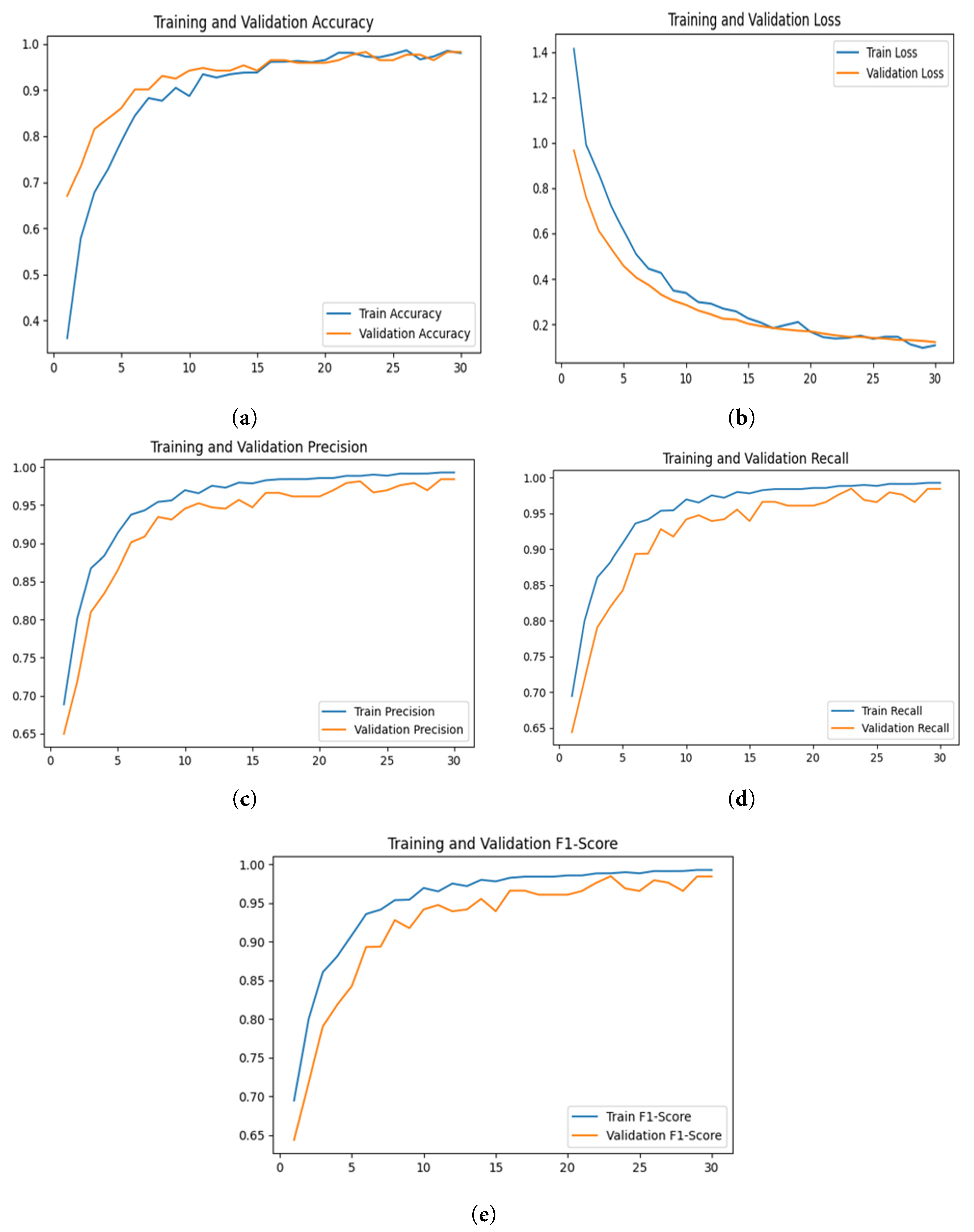
Figure 19: Graphical analysis of the proposed DenseSwinGNNNet model with Adam optimizer based on training and validation. (a) Accuracy, (b) Loss, (c) Precision, (d) Recall, and (e) F1-score.

The confusion matrix depicted in Fig. 20 shows the classification performance of the suggested DenseSwinGNNNet model, trained using the Adam optimizer, demonstrating its high accuracy and stability across four classes: Aphids Disease, Blotch, Healthy Leaf, and Leaf Spot. The model classifies almost all the samples from each class with near-perfect accuracy. For Aphids Disease, 21 out of 22 samples were accurately classified, with only one slight misclassification as Blotch, reflecting the model’s high sensitivity. The Blotch class shows perfect identification, with all 24 samples correctly predicted, reflecting the optimizer’s strength in adjusting learning parameters for precise convergence. In the same vein, both Healthy Leaf and Leaf Spot classes recorded immaculate recognition, with all 19 and 21 samples, respectively, being correctly predicted and no misclassifications. This stable performance indicates the model’s strong feature extraction and improved learning ability with the incorporation of dense connectivity, transformer-based attention, and graph-based reasoning. The application of the Adam optimizer also helped with better gradient stability and faster convergence, minimizing overfitting and enabling smooth optimization. In totality, the confusion matrix verifies that DenseSwinGNNNet with the Adam optimizer holds superior generalization and classification performance, hence being a resourceful and trustworthy framework for smart agricultural disease diagnosis and precision crop monitoring.

Figure 20: Confusion matrix of the DenseSwinGNNNet model with Adam optimizer evaluated on the held-out 10% test set, illustrating correct and misclassified samples for the four turmeric leaf disease classes.

The performance test of the optimized DenseSwinGNNNet model, using the Adam optimizer as presented in Table 8, exhibits impressive classification ability across all categories of tea leaves, with near-perfect precision, recall, and F1-scores. For the Aphids Disease class, the model achieved 100% precision, 99% recall, and an F1-score of 98%, reflecting highly reliable predictions with only one minor incorrect classification. The Blotch class attained 98% precision and 100% recall with an F1-score of 99%, which indicates the model’s capability to identify all actual Blotch samples without false positives. The Healthy Leaf and Leaf Spot classes attained a perfect score of 100% precision, recall, and F1-score, affirming the model’s strength in accurately identifying both healthy and diseased samples. The 99.7% generalization and learning stability reflect the powerful capabilities of the Adam optimizer, which efficiently improves gradient convergence and avoids overfitting. DenseNet’s feature reuse, Swin Transformer’s self-attention for global context, and GNN’s relational learning, combined, enable DenseSwinGNNNet to identify intricate spatial and textural information with higher accuracy. These findings together confirm that the Adam-optimized DenseSwinGNNNet model achieves top-notch performance and is highly efficient and reliable for automatic plant disease detection and precision agriculture use.

The ROC curve of the designed DenseSwinGNNNet model for the turmeric leaf disease classification, as illustrated in Fig. 21, clearly depicts the enhanced discriminative ability of the model for four classes. The ROC curve graphically represents the true positive rate vs. the false positive rate for each class, providing a global measure of how well the model can differentiate between diseased and healthy leaves. The AUC scores for all four classes are 0.99, which is very close to perfect classification power. The high value of AUC clearly demonstrates that the model effectively discriminates among the four classes with minimal misclassification. The sharp slope of the curves towards the top-left corner indicates that the model has high recall with minimal false positives. The improved classification result stems from the analysis conducted using the Adam optimizer on the presented model, which enables effective decision-making. The AUC scores validate the robustness of the model in practical applications where high sensitivity is crucial for accurately detecting diseased turmeric leaves with few false alarms. The fact that different classes’ ROC curves are so close to one another indicates an evenly balanced model with no strong bias towards any particular class, which also verifies its generalization capability. The outcome of the ROC curve validates the precision of the model developed to apply in precision agriculture as an effective method for early detection and categorization of leaf turmeric disease, with the potential for improved crop management and yield increase.

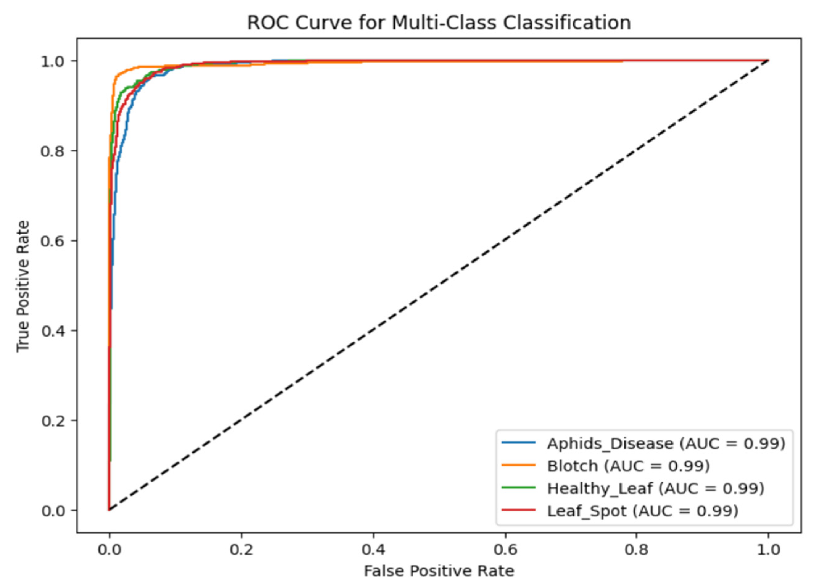
Figure 21: Analysis of the proposed DenseSwinGNNNet model with Adam optimizer based on ROC curve.

4.7 Five-Fold Cross-Validation Results

The five-fold cross-validation results shown in Table 9 also prove the robustness and generalization power of the introduced DenseSwinGNNNet model. The model performed consistently high classification performance in all five folds, with an accuracy between 99.2% to 99.6% and an average mean accuracy of 99.4% ± 0.2%. Correspondingly, the precision, recall, and F1-score metrics were extremely consistent with average values of 99.5%, 99.3%, and 99.4%, respectively, and minimal standard deviation over folds. This reinforces that the model’s performance does not hinge on any fixed data split and that it stays in high discriminative capacity under different training–testing partitions. The small variance across the folds suggests good generalization and robustness, effectively eliminating overfitting or performance inflation due to an advantageous division of data. These results provide strong empirical support for DenseSwinGNNNet’s robust learning mechanism, which consistently achieves high accuracy and resilience across various test scenarios, thereby enhancing the credibility of its reported 99.7% classification accuracy.

Beyond its classification accuracy, the proposed model exhibits potential for secure deployment under adversarially resilient configurations. Integrating adversarial training and differential privacy mechanisms can enhance model robustness and mitigate risks from malicious perturbations or data inference attacks. These measures ensure that the model’s decisions remain stable and reliable even in the presence of noisy or manipulated data.

5 Ablation Analysis

The ablation study presented in Table 10 demonstrates the model’s improved performance with the progressive addition of various architectural elements, highlighting the efficiency of the developed DenseSwinGNNNet model. The baseline DenseNet121 model achieved an average precision of 90.5%, a recall of 90.2%, an F1-score of 90.2%, and an overall accuracy of 91.0%. Its robust feature extraction ability via dense connectivity is evident, but it lacks contextual information. When the Swin Transformer was combined with DenseNet121, performance was significantly enhanced. The average precision, recall, and F1-score increased to 93.7%, 93.5%, and 93.5%, respectively, while accuracy reached up to 94.0%. This improvement is due to the Swin Transformer’s hierarchical attention mechanism, which captures local and global dependencies, enhancing feature representation. Lastly, the Proposed DenseSwinGNNNet model, which incorporates GNNs for learning relationships, performed spectacularly, achieving 99.5% precision, recall, and F1-score, and 99.7% accuracy, indicating nearly perfect classification. Adding GNN modules allows effective modeling of relationships between classes as well as spatial correlations among leaf features, resulting in better discrimination and resilience. In summary, the ablation study effectively confirms that each architectural improvement—dense connections, Transformer-based attention, and GNN relational learning—makes a synergistic contribution toward achieving state-of-the-art performance in plant disease classification.

6 State-of-the-Art Analysis

Previous studies on turmeric leaf disease detection, summarized in Table 11, reveal a gradual evolution from traditional machine learning to deep hybrid architectures. Early models such as VGG16 and VGG19 [19] achieved accuracies between 93–97% on manually collected datasets but were limited to basic convolutional feature extraction without hierarchical or contextual understanding. Classical machine learning approaches using Logistic Regression, KNN, and SVM [16] achieved around 92% accuracy but relied heavily on handcrafted features, restricting adaptability to complex field images.

In contrast, the proposed DenseSwinGNNNet integrates DenseNet121, Swin Transformer, and GNN in a unified, end-to-end framework that jointly learns local, global, and relational features. This design enables deeper spatial reasoning and stronger generalization, achieving an impressive 99.7% accuracy on the turmeric leaf disease dataset. The model’s performance was further validated through five-fold cross-validation and significance testing (p < 0.05), confirming its robustness. Other works, including CNN and InceptionV3-based models [4], and DenseNet201 with machine learning classifiers [5], demonstrated strong performance but were constrained by the simplicity of the dataset or non-leaf applications. Ensemble methods like SVM, Random Forest, and XGBoost [14] reached 93% accuracy yet lacked spatial feature integration. In contrast, the proposed DenseSwinGNNNet framework integrates DenseNet121, Swin Transformer, and GNN in an end-to-end architecture, combining convolutional, attention-based, and relational learning to achieve 99.7% accuracy with superior generalization, interpretability, and scalability over prior state-of-the-art models.

The performance comparison summarized in Table 11 involves studies conducted on diverse datasets collected under different environmental and imaging conditions. Therefore, the reported accuracy metrics should not be viewed as direct measures of superiority. The comparison primarily highlights the architectural evolution and methodological innovations within the field, rather than absolute performance ranking. Despite this variability, the proposed DenseSwinGNNNet demonstrates consistently high results and robust cross-validation performance, underscoring its strong generalization capability and potential scalability to broader agricultural disease classification tasks.

7 Conclusion

In this study, the proposed DenseSwinGNNNet model successfully combines DenseNet121, Swin Transformer, and GNN to attain a strong and accurate solution to disease classification of turmeric leaf. The enhanced performance of the model, with a general accuracy rate of 99.7% and consistently high precision, recall, and F1-score values of 99.5%, respectively, confirms its strength in classifying Aphids Disease, Blotch, Leaf Spot, and Healthy Leaf. The hybrid architecture leverages the feature extraction capability of DenseNet121, the hierarchical spatial pattern recognition of Swin Transformer, and the modeling of complex feature relationships by GNN, all of which enhance the model’s generalization and classification abilities. Low reported misclassifications in the confusion matrix and high AUC scores also support the credibility of the model. The entire preprocessing pipeline of the research and strategic data augmentation ensured effective training and validation to avoid the risk of overfitting. By enabling accurate and early leaf disease detection, the DenseSwinGNNNet model is a valuable tool in precision agriculture, allowing farmers to embrace timely disease control and stem crop loss. Subsequent research could explore real-time deployment of the model on edge computing devices to facilitate feasible use in field disease detection and monitoring. The work represented herein is part of the grand effort to incorporate AI-based solutions into sustainable agricultural practices, aiming to enhance food security and farmers’ economic stability.

References

1. Subramanian M , Gantait S , Jaafar JN , Ismail MF , Sinniah UR . Micropropagation of white turmeric (Curcuma zedoaria (Christm.) Roscoe) and establishment of adventitious root culture for the production of phytochemicals. Ind Crops Prod. 2025; 223: 120101. doi:10.1016/j.indcrop.2024.120101. [Google Scholar] [CrossRef]
2. Albattah W , Javed A , Nawaz M , Masood M , Albahli S . Artificial intelligence-based drone system for multiclass plant disease detection using an improved efficient convolutional neural network. Front Plant Sci. 2022; 13: 808380. doi:10.3389/fpls.2022.808380. [Google Scholar] [CrossRef]
3. Lekbangpong S , Ratanachai A . Technology Transfer needs assessment for turmeric farmers in Paphayom District, Phatthalung Province: prodution, problems and needs of farmers for technology transfer to do turmeric production in Paphayom District, Phatthalung Province. ASEAN J Sci Technol Rep. 2024; 28( 1): e254806. doi:10.55164/ajstr.v28i1.254806. [Google Scholar] [CrossRef]
4. Chathurya C , Sachdeva D , Arora M . Real-time turmeric leaf identification and classification using advanced deep learning models: initiative to smart agriculture. In: Hassanien AE , Anand S , Jaiswal A , Kumar P , editors. Innovative computing and communications. Singapore: Springer Nature; 2024. p. 657– 69. doi:10.1007/978-981-97-3817-5_46. [Google Scholar] [CrossRef]
5. Siam AKMFK , Nirob MAS , Bishshash P , Assaduzzaman M , Ghosh A , Noori SRH . A data-driven approach to turmeric disease detection: dataset for plant condition classification. Data Brief. 2025; 59: 111435. doi:10.1016/j.dib.2025.111435. [Google Scholar] [CrossRef]
6. Selvaraj R , Geetha Devasena MS . A novel attention based vision transformer optimized with hybrid optimization algorithm for turmeric leaf disease detection. Sci Rep. 2025; 15( 1): 17238. doi:10.1038/s41598-025-02185-7. [Google Scholar] [CrossRef]
7. Devisurya V , Devi Priya R , Anitha N . Early detection of major diseases in turmeric plant using improved deep learning algorithm. Bull Pol Acad Sci Tech Sci. 2022; 70( 2): 140689. doi:10.24425/bpasts.2022.140689. [Google Scholar] [CrossRef]
8. Vinayarani G , Prakash HS . Growth promoting rhizospheric and endophytic bacteria from Curcuma longa L. as biocontrol agents against rhizome rot and leaf blight diseases. Plant Pathol J. 2018; 34( 3): 218– 35. doi:10.5423/PPJ.OA.11.2017.0225. [Google Scholar] [CrossRef]
9. Singh G , Al-Huqail AA , Almogren A , Kaur S , Joshi K , Singh A , et al. Enhanced leaf disease segmentation using U-Net architecture for precision agriculture: a deep learning approach. Food Sci Nutr. 2025; 13( 7): e70594. doi:10.1002/fsn3.70594. [Google Scholar] [CrossRef]
10. Sharma R , Sharma A , Hariharan S , Mahajan S . Implementing convolutional neural networks and AdaBoost for varied turmeric discrimination in India. In: Proceedings of the 2024 IEEE International Conference on Information Technology, Electronics and Intelligent Communication Systems (ICITEICS); 2024 Jun 28–29; Bangalore, India. p. 1– 5. doi:10.1109/ICITEICS61368.2024.10625183. [Google Scholar] [CrossRef]
11. Mervin Paul Raj M , Vijayakumar J . Turmeric farm monitoring and automation using deep learning and fuzzy logic on raspberry Pi: a low-cost and energy efficient solution. In: Proceedings of the 2024 Fourth International Conference on Advances in Electrical, Computing, Communication and Sustainable Technologies (ICAECT); 2024 Jan 11–12; Bhilai, India. p. 1– 8. doi:10.1109/ICAECT60202.2024.10469659. [Google Scholar] [CrossRef]
12. Lanjewar MG , Asolkar SS , Parab JS . Hybrid methods for detection of starch in adulterated turmeric from colour images. Multimed Tools Appl. 2024; 83( 25): 65789– 814. doi:10.1007/s11042-024-18195-y. [Google Scholar] [CrossRef]
13. Selvaraj R , Geetha Devasena MS , Satheesh T , Sathishkumar C . AI for smart agriculture–a deep learning based turmeric leaf disease detection. In: Proceedings of the 2024 9th International Conference on Communication and Electronics Systems (ICCES); 2024 Dec 16–18; Coimbatore, India. p. 1491– 5. doi:10.1109/ICCES63552.2024.10859805. [Google Scholar] [CrossRef]
14. Tanwar V , Anand V , Chauhan R , Rawat RS , Kumar GR . Enhanced classification of turmeric leaf disease severity levels using an optimized hybrid deep learning model: LevelPrecisionRecallF1-scoreAccuracy. In: Proceedings of the 2024 International Conference on E-mobility, Power Control and Smart Systems (ICEMPS); 2024 Apr 18–20; Thiruvananthapuram, India. p. 1– 5. doi:10.1109/ICEMPS60684.2024.10559345. [Google Scholar] [CrossRef]
15. Lanjewar MG , Parate RK , Wakodikar R , Parab JS . Detection of starch in turmeric using machine learning methods. In: Kumar S , Sharma H , Balachandran K , Kim JH , Bansal JC , editors. Third congress on intelligent systems. Singapore: Springer Nature; 2023. p. 117– 26. doi:10.1007/978-981-19-9379-4_10. [Google Scholar] [CrossRef]
16. Senthil Pandi S , Kumar P , Salman Latheef TA . Projection of plant leaf disease using support vector machine algorithm. In: Proceedings of the 2023 International Conference on Recent Advances in Science and Engineering Technology (ICRASET); 2023 Nov 23–24; B. G. Nagara, India. p. 1– 6. doi:10.1109/icraset59632.2023.10419981. [Google Scholar] [CrossRef]
17. Nawaz M , Nazir T , Khan MA , Rajinikanth V , Kadry S . Plant disease classification using VGG-19 based faster-RCNN. In: Singh M , Tyagi V , Gupta PK , Flusser J , Ören T , editors. Advances in computing and data sciences. Cham, Switzerland: Springer Nature; 2023. p. 277– 89. doi:10.1007/978-3-031-37940-6_23. [Google Scholar] [CrossRef]
18. Velmurugan S , Ramdinesh Reddy K , Rahul SG , Vardhan S , Subitha D , Vignesh SK . A comparative computational analysis of VGG16 and VGG19 in prediction of turmeric plant disease. In: Proceedings of the 2022 8th International Conference on Advanced Computing and Communication Systems (ICACCS); 2022 Mar 25–26; Coimbatore, India. p. 130– 4. doi:10.1109/icaccs54159.2022.9784970. [Google Scholar] [CrossRef]
19. Janani V , Siva Mangai NM . Analysis and classification of rhizome rot disease for turmeric plant using artificial intelligence. In: Proceedings of the 2022 International Conference on Sustainable Computing and Data Communication Systems (ICSCDS); 2022 Apr 7–9; Erode, India. p. 411– 4. doi:10.1109/icscds53736.2022.9760884. [Google Scholar] [CrossRef]
20. Mendeley Data . Turmeric Plant Disease Dataset [Dataset]. 2020 [cited 2025 Aug 15]. Available from: https://data.mendeley.com/datasets/jtttfbx342/1 [Google Scholar]
Cite This Article
Copyright © 2025 The Author(s). Published by Tech Science Press.
This work is licensed under a Creative Commons Attribution 4.0 International License , which permits unrestricted use, distribution, and reproduction in any medium, provided the original work is properly cited.
Downloads
Citation Tools