Modeling and Estimating Soybean Leaf Area Index and Biomass Using Machine Learning Based on Unmanned Aerial Vehicle-Captured Multispectral Images

1  Introduction

Estimating crop biophysical parameters such as leaf area index (LAI) and biomass played a vital role in precision agriculture and crop management. Traditionally, field-based LAI sampling and measurements are proven to be challenging and time-consuming. Direct methods, such as leaf collection and area measurement, are not only labor-intensive but also destructive. Similarly, traditional field-based crop biomass measurement entails destructive, laborious and time-consuming procedures. Remote sensing (RS) emerges as a promising indirect solution for reducing crop management cost and improving crop management practices. Utilizing RS for LAI and biomass estimation offers efficiency and effectiveness compared to conventional direct methods. In recent years, Satellite RS has been used for estimating LAI and biomass [1]. However, for field-scale crop study of LAI and biomass estimations RS from unmanned aerial vehicles (UAVs) is more suitable [2–11] and biomass [12–14] for precision crop management. UAV RS data provides high-resolution spatial, spectral, and temporal data at a relatively low cost [12].

Leaves play a crucial role in crops, impacting photosynthesis, growth, and yield. LAI, defined as the ratio of one-sided leaf area to the ground area, is an important agroecological factor and serves as a measure of crop growth. LAI helps the quantification of sunlight interception by plants, directly affecting photosynthesis and evapotranspiration, thus serving as a fundamental indicator of crop growth [8]. It holds significance in influencing crop production and assessing crop growth status [2]. Furthermore, LAI proves valuable in detecting prolonged water stress, estimating biomass, and identifying crop growth stages [10]. Crop biomass is another important agroecological factor also which is defined as the total amount of organic matter produced by a crop during its growth cycle, encompassing all plant materials, including stems, leaves, roots, and any harvested portions like grains or fruits, to indicate crop growth status and physiological conditions [12]. It is used to assess crop health status, nutrient supply and necessity of agricultural management practices [14].

Various crops exhibit distinct patterns in the relationships among LAI, biomass, and Vegetation Indices (VIs). For instance, rice demonstrated a less significant correlation between LAI and VIs throughout its growth stages due to differing canopy spectra and structure [2]. In contrast, peanut LAI displayed a strong correlation with VIs derived from UAVs [3]. Sunflower LAI exhibited a notable correlation with UAV-derived NDVI (Normalized Difference Vegetation Index) [4]. Additionally, UAV-captured RGB images proved effective in estimating LAI for winter wheat [5]. Maize LAI estimation utilized multimodal data derived from UAVs [7]. Cumulative VIs demonstrated enhanced performance in corn LAI estimation [11]. Furthermore, crop biomass was estimated using VIs derived from UAVs. For instance, soybean biomass was estimated using VIs within a weighted canopy volume model, considered simple yet effective [12]. Rice biomass was also measured using UAV-derived VIs at various growth stages [13]. A combination of VIs and plant height was employed to estimate barley biomass [14]. Alternative satellite sensors, such as RapidEye multispectral data, were also utilized for estimating LAI and biomass in soybean and corn [11].

For crop growth and yield monitoring, there are several VIs derived from UAV or satellite-captured multispectral data. For instance, 14 VIs were applied to soybean yield estimation studies, which showed a reliable estimation ability [15]. Also, an overview of 20 VIs based on the visible near-infrared spectrum was reported and extensively used for monitoring vegetation conditions, such as health, growth levels, productivity, water and nutrients stress [16]. Moreover, canopy reflectance could differ between crops of different canopy structures even when they have the same canopy chlorophyll content [17]. Therefore, accuracy in measuring LAI is an important factor in indirect methods. Recently, UAV derived 3D-point cloud-based method applied for LAI mapping, which will reduce the necessity of ground-based measurement [18].

Estimation of biomass from VIs also varied based on sensors. In a study, satellite imagery-derived VIs were used to estimate wheat yield and biomass [19]. Based on the crop types the VIs also showed different patterns of biomass estimation. For pasture biomass estimation, Atmospherically Resistant Vegetation Index (ARVI) showed most reliability [20]. Biomass estimation on rangeland showed that grazed sites were correlated to VIs, but ungrazed sites had no significant relation [21]. For barley biomass, the combination of plant height with VIs showed good correlation [22]. In pasture biomass estimation, Modified Normalized Difference Vegetation Index (MNDVI), Simple Ratio (SR) and Transformed Vegetation Index (TVI) were used and compared with NDVI [23].

Machine learning (ML) algorithms played a pivotal role in estimating crop LAI and biomass. For instance, the optimal regression method was used to forecast peanut LAI [3], and a regression-based approach was employed to determine sunflower LAI using UAV-derived NDVI [4]. Univariate and multivariate regression models were applied to ascertain LAI in winter wheat along with deep neural networks [4–7]. The regression models for LAI estimation using Cubist and Random Forests (RF) methods with VIs derived from Landsat 8 imagery were proposed [24], and the XGBoost modeling method, combined with competitive adaptive reweighed sampling and successive projections (CARS-SPA) algorithm, demonstrated efficiency in winter wheat LAI estimation [25]. Feature selection and three ML algorithms—RF, backpropagation neural network (BPNN), and K-nearest neighbor (KNN) were also utilized for LAI estimation [26]. Linear regression (LR), BPNN, and RF were applied to digital images from UAV platforms equipped with complementary metal-oxide-semiconductor (CMOS) image sensors for maize LAI estimation [8]. Simple LR, Multiple Linear Regression (MLR), RF, XGBoost, Support Vector Machine (SVM), and BPNN were employed for soybean LAI measurement from hyperspectral, multispectral and LiDAR data acquired on UAVs [27]. WorldView-2 satellite imagery proved effective for estimating LAI of grasslands and forests using ML models such as BPNN, RF, and SVM [28]. Deep learning (DL) fused with RGB images was used to estimate rice LAI [6], and Landsat satellite imagery with 30 m resolution was applied for LAI estimation [29]. These ML models were also utilized for crop biomass estimation. For seasonal corn biomass estimation, RF, SVM, artificial neural network (ANN), and XGBoost showed efficiency [30]. Automated machine learning (AutoML) technology was applied for crop biomass estimation [31], and RF, SVR, ANN, and partial least squares (PLS) were utilized for oats [32] and maize [33] biomass estimations. Canola, corn, and soybean biomass were monitored using SVR and ANN models [34]. Additionally, biomass estimation for other crops such as rice [35], wheat [36], and potato [37] was conducted using ML models. ML is part of artificial intelligence, which is capable of modeling the process without the need to assume the form of the model to “outperform” regular statistical approaches. However, it is noted that the statistical regression approaches still work well in some cases, instead of using ML approaches with computing complexity. An example is shown in the work of Lao et al. [38] in which the retrieval of chlorophyll content for vegetation communities under different inundation frequencies performed well using simple linear regression and partial least squares based on the VIs extracted from UAV images and field canopy chlorophyll, leaf chlorophyll and LAI measurements.

Soybeans are a leguminous crop that has a growth cycle of 120 to 150 days. The growth stages are classified into vegetative and reproductive. Therefore, we explored some previously reported VIs to study soybean biophysical parameters. We have closely monitored the reproductive stages to measure soybean LAI and biomass condition from RS method. In this study, we adopted widely used ML approaches, i.e., LR, RF, and SVM. These methods were easily applicable and reliable. This study will help to identify and summarize the useful VIs to estimate soybean LAI and biomass in reproductive phases. This study will add information for agricultural crop management through RS to benefit the national economy from agricultural production.

2  Experimental Design and Methodology

2.1 Study Site

The study site was located near Pontotoc, MS, USA in the farm of the Pontotoc Ridge-Flatwoods Branch Experiment Station (34.2478831°N, 88.998673°W) of Mississippi Agricultural and Forestry Experiment Station (MAFES) (Fig. 1). It is situated in the humid subtropical climate zone. The temperature ranges between 30–35°C during day and 20–23°C at night during the summer period. The monthly average precipitation often ranges from about 4 to 5 inches (approximately 100 to 130 mm) in the summer.

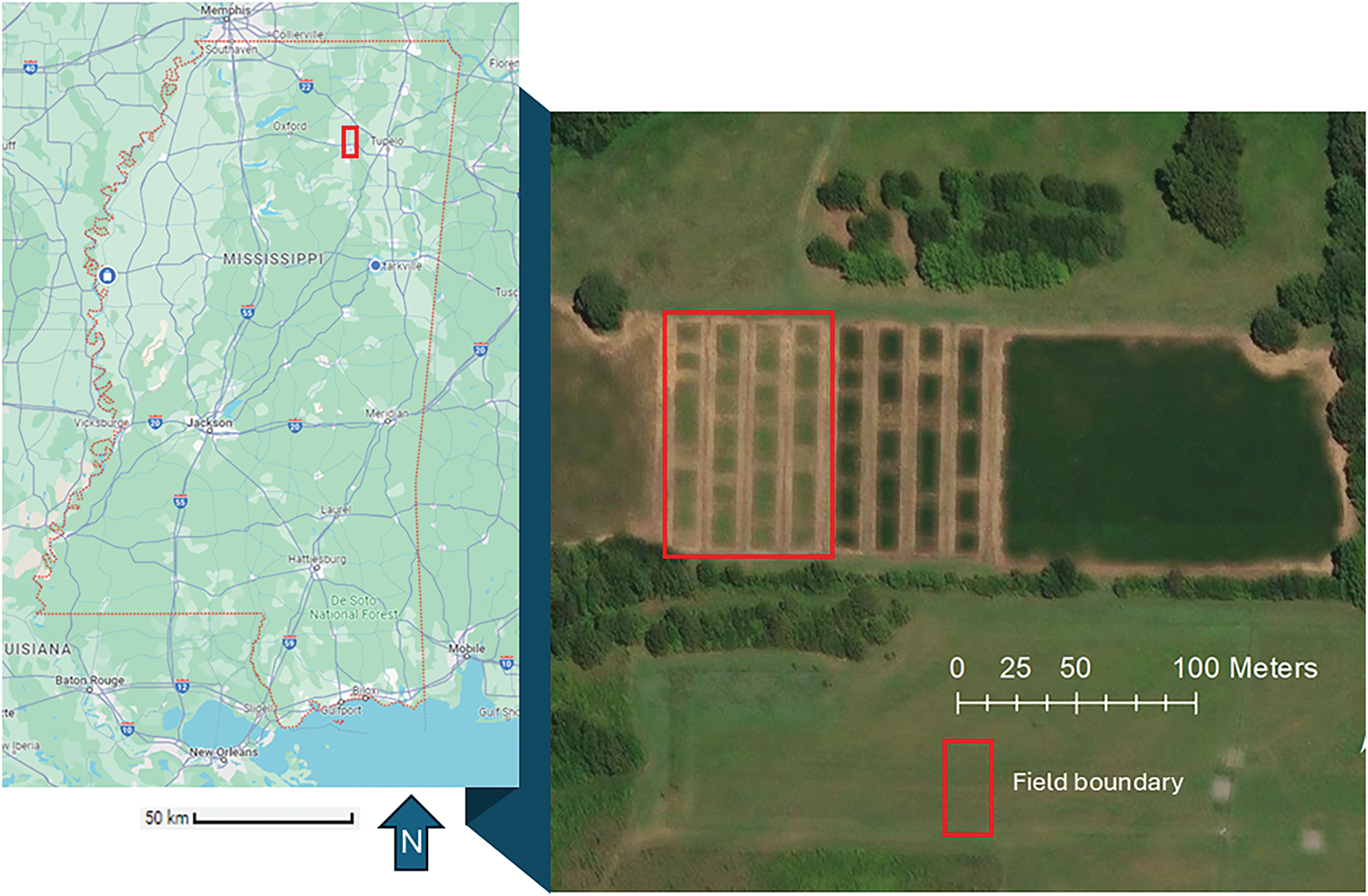
Figure 1: The soybean experiment field in the study site

2.2 Field Experiment and Data Collection

The experiment was conducted in the 2022 soybean growth season (April–September). We monitored soybean biophysical parameters, including LAI and biomass, focusing on the reproductive stages.

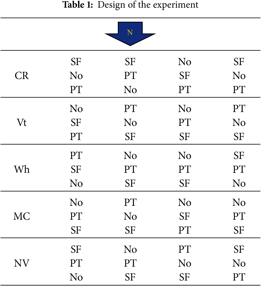
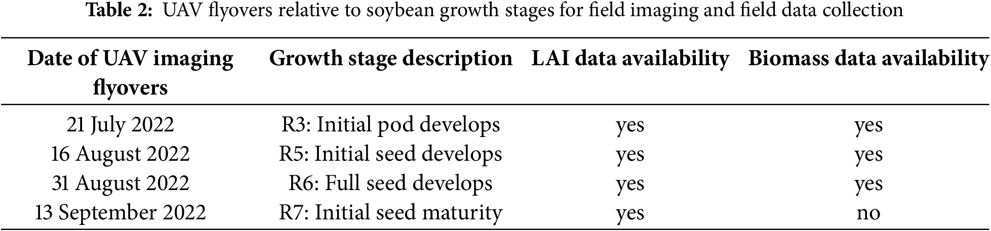
The experiment was designed to include five cover crops (CR: Cereal Rye, Vt: Vetch, Wh: Wheat, MC: Mustard plus Cereal Rye, and NV: native vegetation) planted in the fall of 2021 and three fertilizer treatments (SF: Synthetic Fertilizer, Pt: Poultry Litter, and No: None) applied before planting the soybean in a full factorial combination. The cover crops were planted to main plots and terminated two weeks before planting soybean in the spring of 2022. This experiment followed a randomized block design, which is shown in Table 1. The size of each plot was 6.1 m by 9.1 m. The synthetic fertilizer treatments were recommended based on standard soil test: 125 kg ha−1 (kilogram per hectare) of Phosphorous (P), 45 kg ha−1 of K (Potassium), 22.4 kg ha−1 of S (Sulphur), and 4.5 kg ha−1 of Zn (Zinc). Poultry litter (PL) at 4500 kg ha−1 was used as a substitute for synthetic fertilizers. The soybean was not irrigated. Table 2 shows the critical reproductive stages with biophysical parameters examined with UAV imaging.

2.3 UAV Imaging

UAV imaging data were collected with five flyovers at different reproductive stages of soybean growth (Fig. 2). The UAV images were acquired using a DJI Phantom 4 quadcopter with a built-in multispectral camera (DJI, Shenzhen, China). On the UAV, the camera was mounted on a gimble with a −90° to +30° tilt controllable range, with six 1/2.9″ 2.08 MP CMOS sensors with a 1600 × 1300 image size and 62.7° field of view. The sensors included one broadband RGB sensor for visible light imaging and five multispectral narrowband monochrome sensors for blue band (B)—450 nm ± 16 nm, green band (G)—560 nm ± 16 nm, red band (R)—650 nm ± 16 nm, red edge band (RE)—730 nm ± 16 nm, and near-infrared band (NIR)—840 nm ± 26 nm). Image radiometric calibration was conducted for converting the images from digital counts to percent reflectance by imaging a calibrated panel with nominal reflectance prior to and after each flight. The camera operation was synchronized for global positioning coordinates with the global navigation satellite system (GNSS; GPS + GLONASS + Galileo) built-in on the UAV. The UAV flights were conducted between 10:30 a.m. and 12:00 p.m. to avoid cloud shadows, as weather permitted in clear days, with a flight altitude of 50 m above the canopy surface to acquire high-resolution (~4 cm/pixel) images along the progress of the soybean’s growth. The flight altitude was consistent at 30 m and 80% frontal overlap and 70% side overlap were set for consecutive imaging. Flight routes were preset using the mission planning tool of Pix4DCapture software (Pix4D, Lausanne, Switzerland). After flight, the images were downloaded to the computer to conduct the pre-processing of the multispectral images using Pix4Dmapper (Pix4D, Lausanne, Switzerland) for orthomosaiking with radiometric and geometric calibrations.

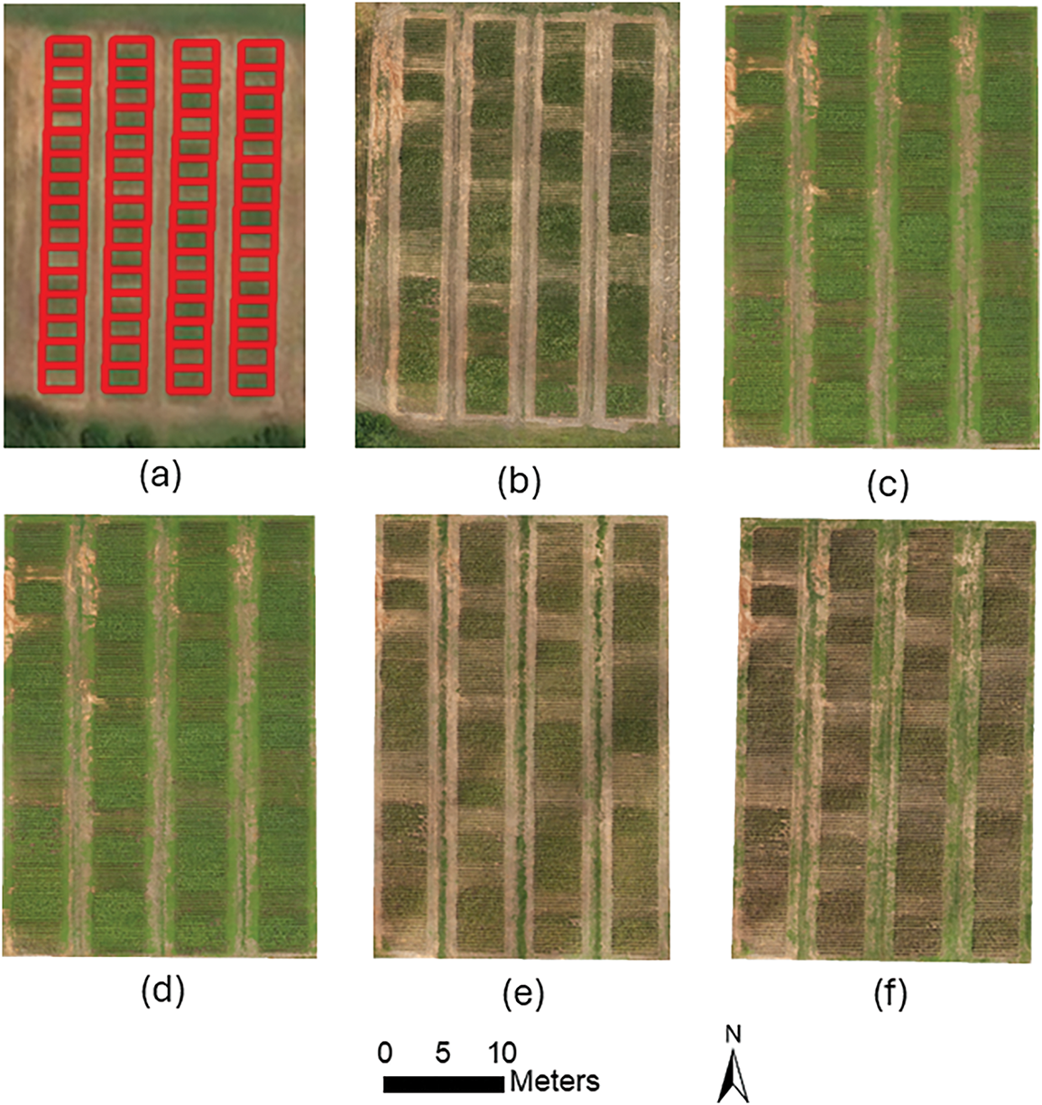
Figure 2: (a) Experimental plot boundary, and the UAV-derived RGB images of the soybean field plot at different reproductive stages, (b) R3: initial pod develops, (c) R4: full pod develops, (d) R5: initial seed develops, (e) R6: full seed develops, and (f) R7: initial maturity

2.4 Vegetation Indices and Biophysical Parameters

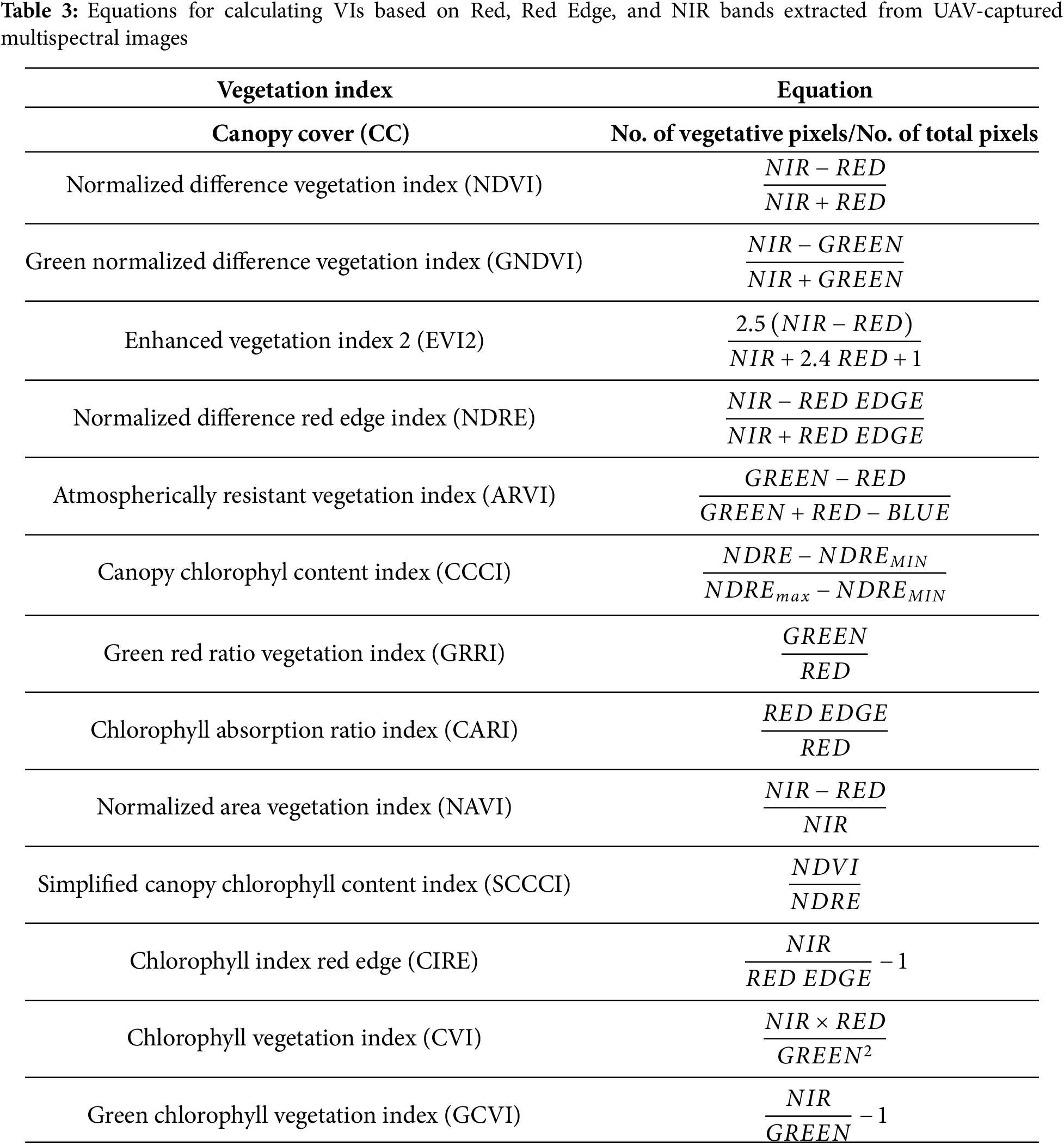
In this study, we made fourteen VIs from collected UAV multispectral images, followed by Shammi et al. [15]. These VIs include canopy cover (CC), normalized difference vegetation index (NDVI), green normalized difference vegetation index (GNDVI), enhanced vegetation index 2 (EVI2), normalized difference red edge index (NDRE), atmospherically resistant vegetation index (ARVI), canopy chlorophyl content index (CCCI), green red ratio vegetation index (GRRI), chlorophyll absorption ratio index (CARI), normalized area vegetation index (NAVI), simplified canopy chlorophyll content index (SCCCI), chlorophyll index red edge (CIRE), chlorophyll vegetation index (CVI), and green chlorophyll vegetation index (GCVI). The mathematical equations of these VIs are included in Table 3.

A Python program was developed with the function to segment vegetation from background for each experimental plot confined by the polygon in the ArcGIS shapefile through thresholding of NDVI values formed by the extracted multispectral band data from the images.

Soybean LAI and biomass were measured in the field at different reproductive growth stages (Table 2). The LAI-2200 plant canopy analyzer (LI-COR Environmental. Lincoln, NE, USA) was used to measure LAI at each plot. This device is a passive sensor used to compute LAI among variety of other canopy structure attributes from radiation measurements above and below canopy. It integrates a fish-eye optical sensor with five silicon detectors arranged in circular rings that sample radiation above and below the canopy at five zenith angles simultaneously. The biomass was determined by the dry weight of five plants collected from each plot dehydrated by an oven to evaporate all moisture from the plants. LAI was measured at R3, R5, R6, and R7 stages and biomass was measured at R3, R5, and R6 stages as shown in Table 2. No other LAI and biomass data were collected due to labor and cost limitations.

2.5 Data Modeling and Evaluation

2.5.1 ML Models

Three commonly used models including linear regression (LR) [4,5,27,28], support vector machine (SVM) [29,32,34,35], and random forest (RF) [24,26–29,32,34,35] were applied for machine learning in this study to evaluate soybean LAI and biomass estimations at the field scale.

LR defines the linear relationship between dependent (responsive) and independent (casual) variables [8]. After testing the data normality using residual analysis, the linear regression method estimates the slope and the intercept of a linear equation to fit the data. SVM enables an optimal hyperplane to minimize the difference between estimated and observed values. It is formed based on structural risk minimization principle and statistical modeling [32]. The Gaussian kernel has been used to map the raw input data to high-dimensional data space. RF is an ensemble machine learning model where many decision trees (DTs) are developed and integrated for accurate classification or estimation results [8]. In this study, we have built 50 independent trees and combined them in a Bagging manner.

The performance of these models, Eqs. (1) and (2) below, is measured by the coefficient of determination (R2) and the Root Mean Square Error (RMSE):

R2=1−SSESST=1−∑(y−y^)2∑(y−y¯)2 (1)

RMSE=∑i=1n(yi^−yi)2n (2)

where y^ is the estimated parameter value, y is the measured parameter value, y¯ is the average parameter value, n is the number of samples, SSE is the sum square error, SST is the total sum square. Both evaluation metrics are widely used in regression analysis to measure model performance. R2, or known as the coefficient of determination, indicates the proportion of variance in the dependent variable explained by the model, ranging from 0 to 1. RMSE measures the average magnitude of errors between predicted and actual values, with lower values indicating better fit. While both indicate how well a model fits the data, R2 focuses on explained variance, while RMSE focuses on prediction accuracy of all regression models for LAI and Biomass estimation in this study.

2.5.2 Leave-One-Out Cross Validation

We used a leave-one-out cross-validation (LOO-CV) method to evaluate the performance of the three regression models: linear regression, SVM regression, and random forest regression. LOO-CV has the advantage of using every data point for both training and testing, making the most out of limited datasets [39]. Unlike methods such as k-fold (k > 1) cross-validation [40], where the data is divided into larger subsets, LOO-CV ensures that every sample is tested exactly once. This makes the evaluation highly accurate and less biased, particularly useful for small datasets where data scarcity is an issue. Specifically, for a dataset with n samples, LOO-CV trains a model on (n − 1) samples and then tests the trained model on the remaining single sample. This process is repeated n times, with each sample serving as the test point once. The final performance metric is obtained by averaging the errors across all test cases. This LOO-CV method ensures a robust estimate of model performance by maximizing the use of available data while avoiding overfitting, as each sample is both a training and test case at different points in the process [41].

We had a limited number of samples in about 60 experimental plots with multiple days of image acquisitions with UAV flyover imaging. So, we used one-leave out cross validation, i.e., the training data will include some samples from the same plot as the test sample, to deal with the limited samples.

3  Results

3.1 Data Exploration and Analysis

3.1.1 LAI and Biomass Estimations

We have explored the ranges of LAI (m2/m2) (Fig. 3a). The range in R3, R5, R6, and R7 stages are 0.5–3.1 (m2/m2), 0.1–4.9 (m2/m2), 1–4 (m2/m2), and 0.8–3.2 (m2/m2), respectively. The maximum LAI observed in R5 stage and the minimum in R7 stage.

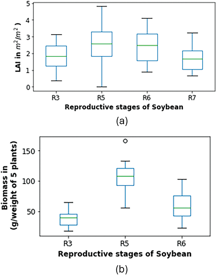
Figure 3: (a) Ranges of LAI at different reproductive stages, i.e., R3, R5, R6, and R7; (b) Ranges of biomass at different reproductive stages, i.e., R3, R5, and R6

The biomass is observed and plotted in Fig. 3b. The ranges of biomass in R3, R5, and R6 stages are about 5–65 (g/weight of 5 plants), 50–175 (g/weight of 5 plants), and 10–110 (g/weight of 5 plants), respectively. The maximum biomass is observed in R5 stage and minimum in R3 stage.

3.1.2 VIs

We have plotted the normalized values of VIs at different reproductive stages, i.e., R3 (Fig. 4a), R5 (Fig. 4b), R6 (Fig. 4c), and R7 (Fig. 4d), respectively. Here, we observe the median values and extent of VIs at the different soybean growth stages.

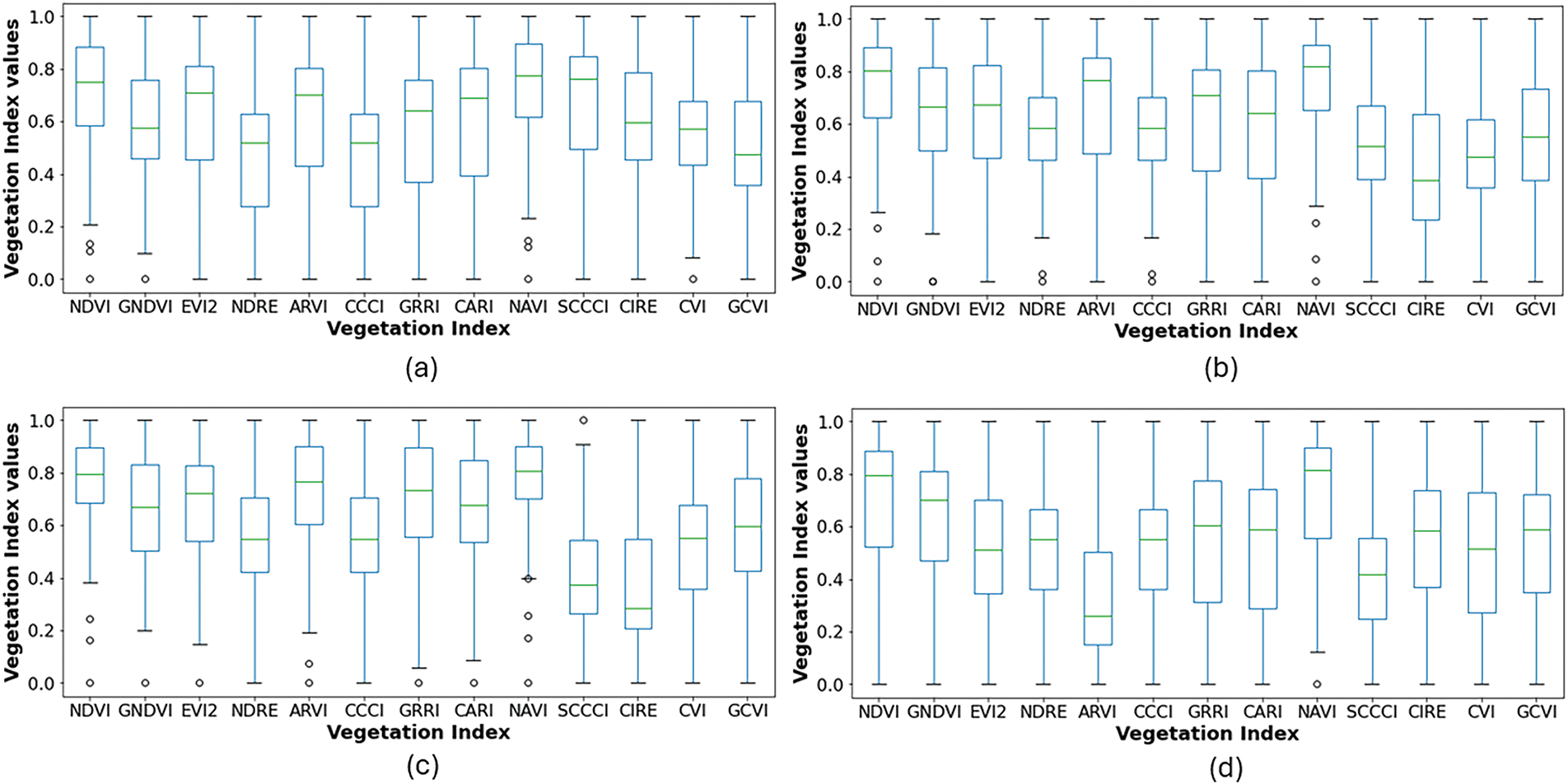
Figure 4: Normalized values of VIs at different reproductive stages, i.e., (a) R3, (b) R5, (c) R6, and (d) R7

3.2 LAI Estimation ML Modeling

According to the ML modeling of LAI, different VIs showed different levels of R2 and RMSE at different reproductive stages. This pattern is plotted in Fig. 5a,b. In R3 stage, CC, NDVI, EVI2, ARVI, GRRI, CARI, NAVI, SCCCI, CIRE showed better estimation ability in all ML models which had R2 about 0.6–0.8 and the RMSE found within 0.2–0.4 (m2/m2). In R5 stage, CC, NDVI, ARVI, GRRI, CARI, NAVI showed about 0.4–0.6 reliability, and RMSE between 0.6 to 0.8 (m2/m2).

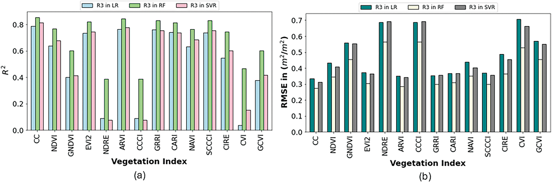
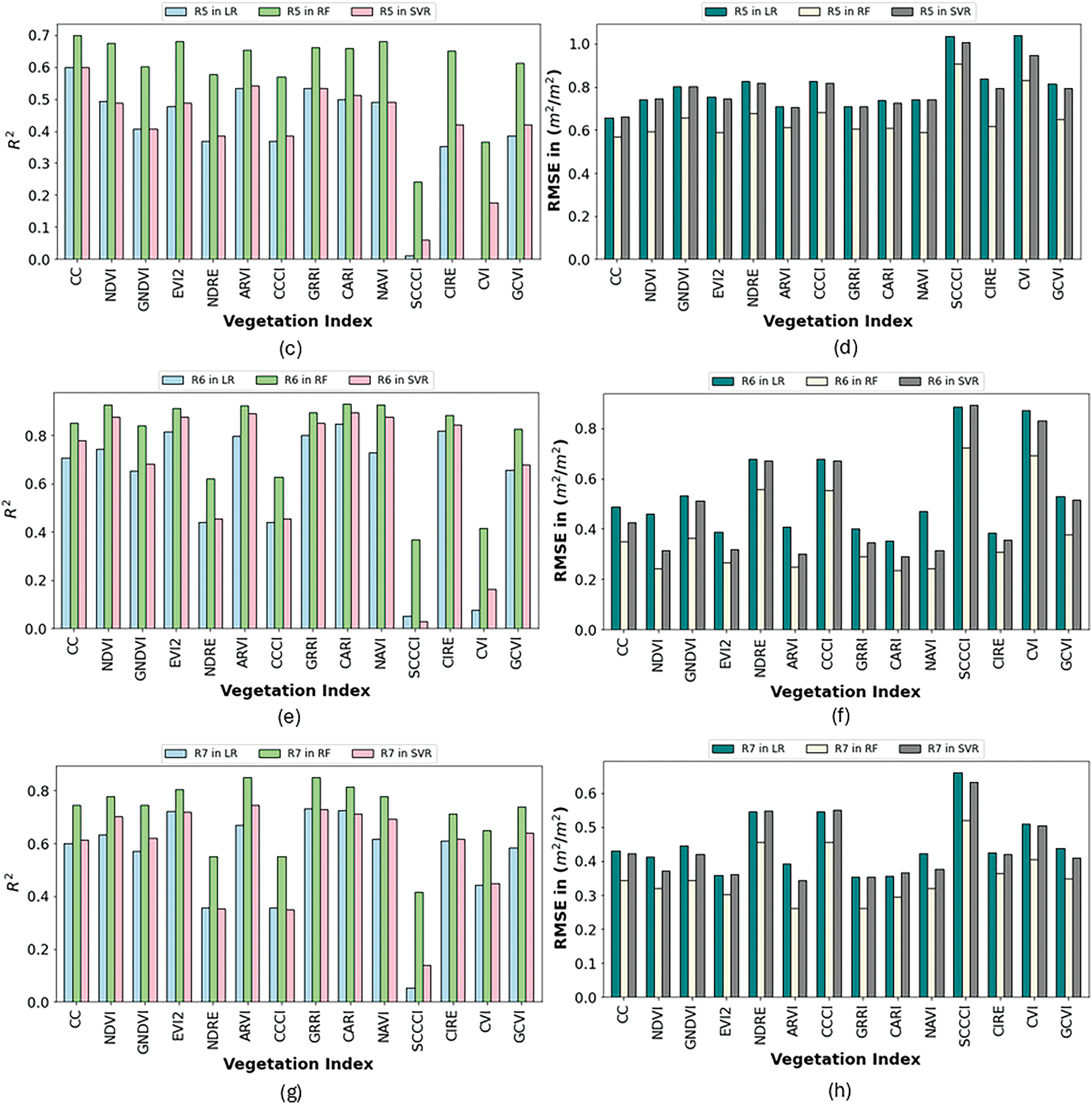
Figure 5: R2 values and RMSE values for R3 stage in (a,b), R5 in (c,d), R6 in (e,f), and R7 in (g,h), respectively, from LAI estimation modeling

In R6 stage, CC, NDVI, EVI2, ARVI, GRRI, CARI, NAVI, CIRE showed better estimation ability where R2 is around 0.8 or above and RMSE is within a range of 0.3 to 0.4 (m2/m2). The R7 stage, EVI2, ARVI, GRRI, CARI, and GCVI showed about R2 at 0.6–0.75 for estimation ability.

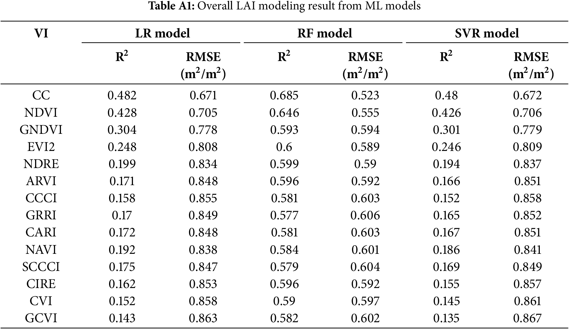
Among the ML models showed consistency in forecasting LAI. Besides, some VIs, i.e., NDRE, CCCI, SCCCI, CVI showed lowest reliability in estimating LAI. Therefore, we also modelled the total reproductive stages using ML models. The results are mentioned in Appendix A Table A1. We found the best estimation ability in RF models with an R2 of 0.5–0.68 and RMSE of 0.52–0.60 (m2/m2). However, the LR and SVR model showed about similar R2 (0.42–0.48) from CC, and NDVI indexes. Overall, the similarity of estimation results observed in both LR and SVR models and best estimation in RF models.

3.3 Biomass Estimation ML Modeling

From ML modeling of crop biomass, the values of R2 and RMSE at different reproductive stages are shown in Fig. 6.

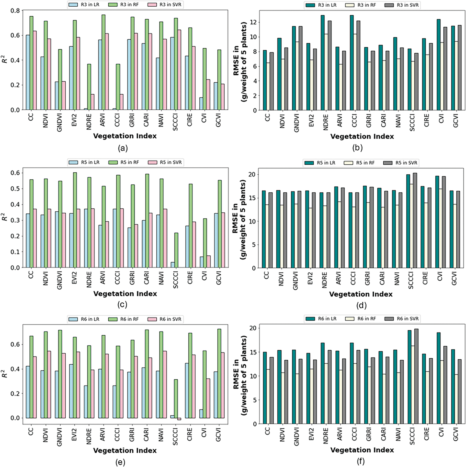
Figure 6: R2 values and RMSE values for R3 stage in (a,b), R5 in (c,d), and R6 in (e,f), respectively, from biomass estimation modeling

At R3 stage, CC, EVI2, ARVI, GRRI, CARI, and SCCCI showed better estimation ability in all ML models, which had an R2 of about 0.6–0.7 and an RMSE found within 6–8 (g/weight of 5 plants). The RF model showed better estimation ability.

At R5 stage, EVI2, ARVI, GRRI, CARI, NAVI, CIRE, and GCVI showed an R2 of about 0.5–0.6 for estimation, and an RMSE within the range of 10 to 15 (g/weight of 5 plants). At R6 stage, CC, EVI2, ARVI, GRRI, CARI, NAVI, CIRE and GCVI showed an R2 between 0.4 to 0.5 for estimation ability where RMSE is within a range of 12 to 15 (g/weight of 5 plants).

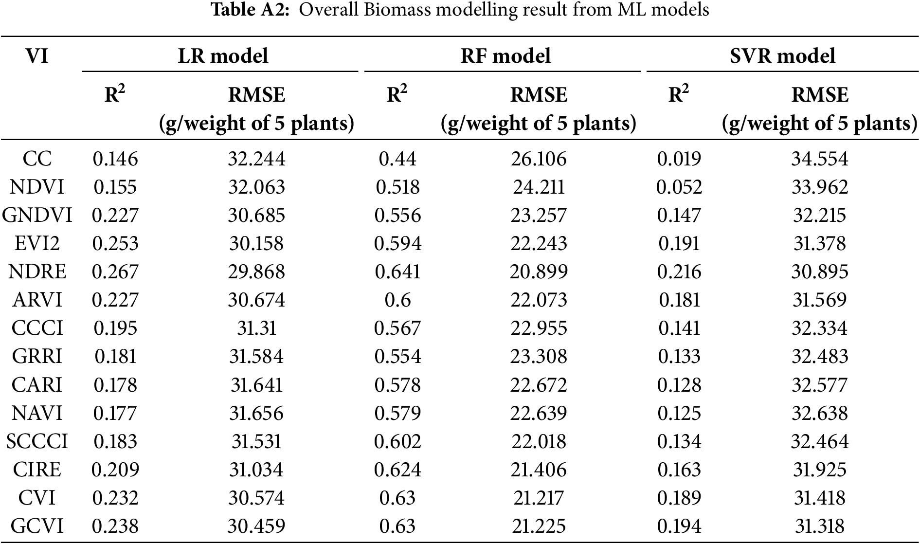
Among the ML models showed consistency in forecasting crop biomass. Also, some VIs, i.e., NDRE, CCCI, and CVI showed lowest reliability in estimating crop biomass. Besides the total reproductive stages modeled by ML models mentioned in Appendix A Table A2. In the LR models, we found that GNDVI, EVI2, NDRE, CIRE, and CVI showed an R2 between 0.20 to 0.27 for estimation whereas in SVR models, EVI2, NDRE, CIRE, CVI, and GCVI showed an R2 of about 0.18–0.22 for estimation. However, the RF models showed an R2 of about 0.44–0.63 for estimation with an RMSE of 20–26 (g/weight of 5 plants). It is considered that RF model estimates crop biomass better than other models.

3.4 Cross-Validated LAI Estimation Modeling

From the cross-validated LAI estimation model by using the fourteen VIs, the levels of R2 and RMSE at different reproductive stages are shown in Fig. 7a,b.

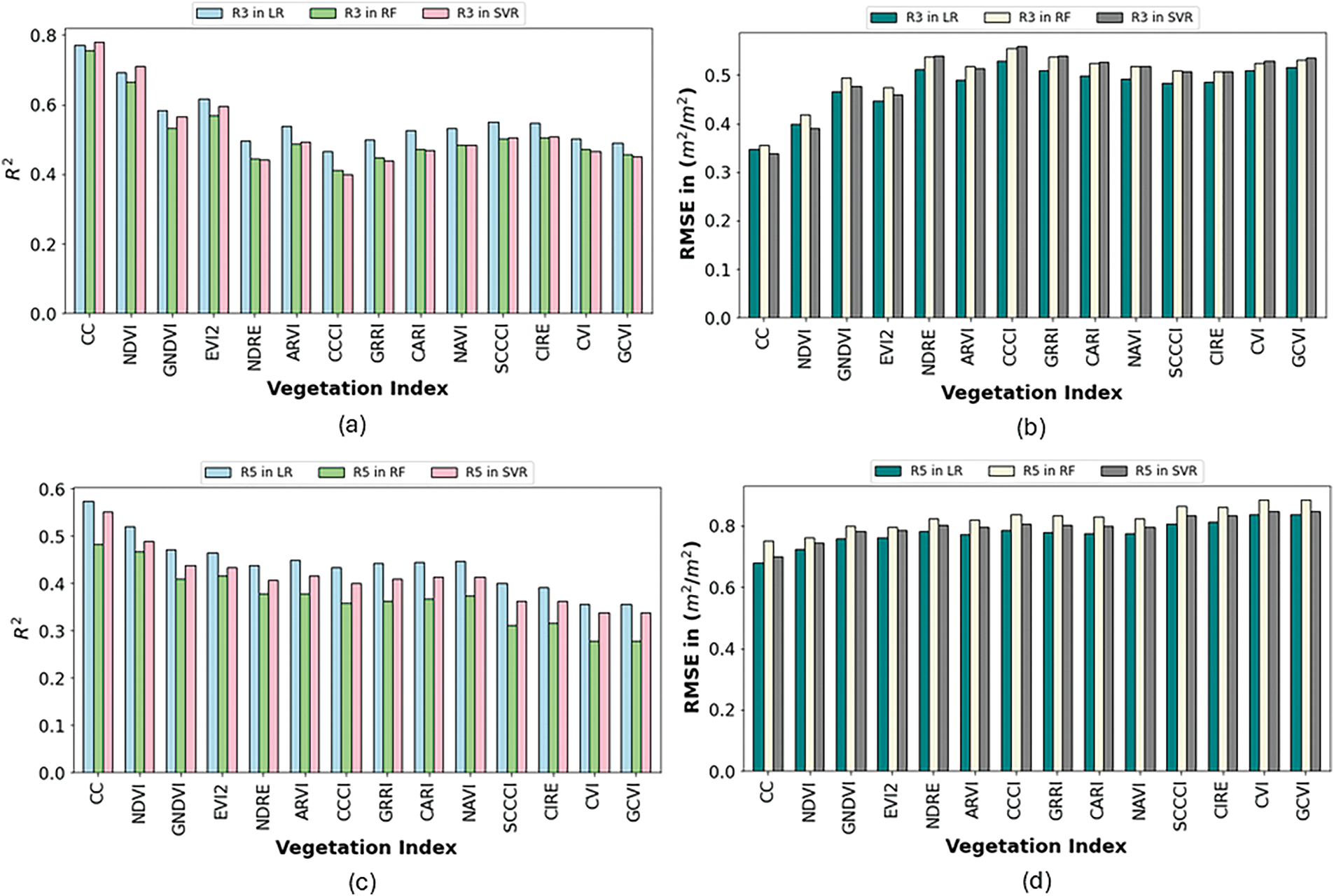
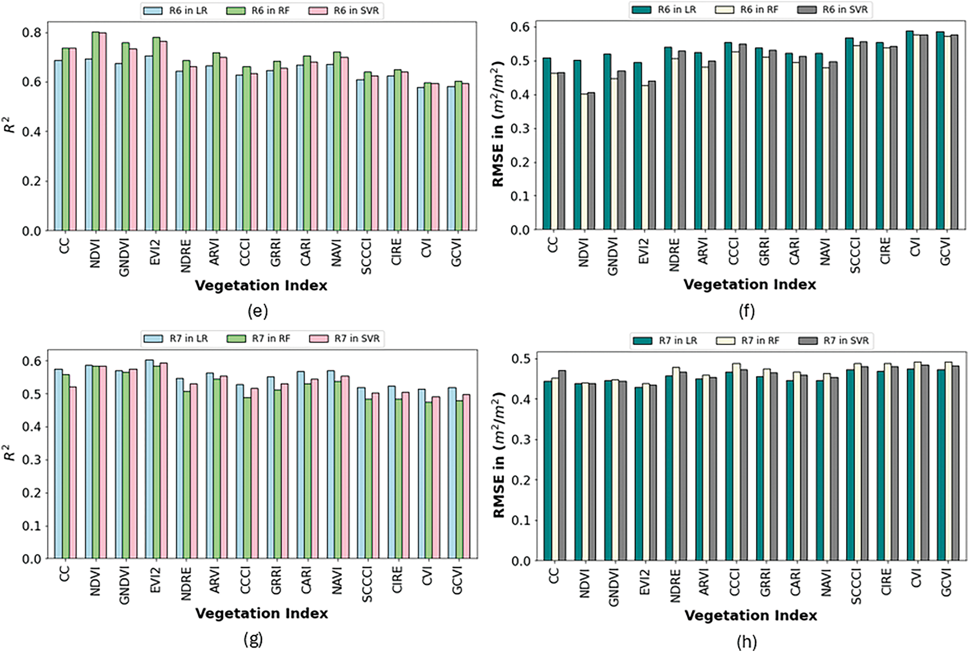
Figure 7: R2 values and RMSE values for R3 stage in (a,b), R5 in (c,d), R6 in (e,f), and R7 in (g,h), respectively, from LAI cross validated estimation modeling

In R3 stage, CC, NDVI, and EVI2 showed better estimation ability in all ML models, which had an R2 of about 0.6–0.8 and the RMSE was found within 0.2–0.4 (m2/m2). In R5 stage, all VIs, showed an R2 of about 0.4–0.6, and RMSE between 0.6 to 0.8 (m2/m2). In R6 stage, CC, NDVI, GNDVI, EVI2, ARVI, GRRI, CARI, NAVI, and CIRE showed an R2 of about 0.7–0.8 estimation ability where RMSE is within a range of 0.4–0.5 (m2/m2). The R7 stage, CC, NDVI, ARVI, GRRI, CARI, and NAVI showed an R2 of about 0.55–0.65 with an RMSE of 0.4–0.6 (m2/m2). Overall, R6 stage showed the best time for LAI estimation from VIs.

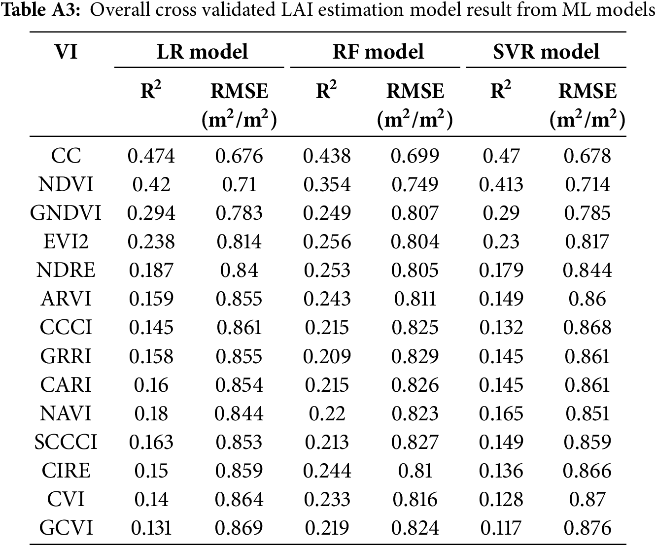
Besides, the modeling of the total reproductive stages of LAI is mentioned in Appendix A Table A3. We found the estimation ability in RF models with an R2 of 0.25–0.44 and RMSE of 0.65–0.85 (m2/m2). The SVR model showed an R2 of about 0.23–0.47 from CC, NDVI, GNDVI, EVI2 indexes, whereas the RMSE are within the range of 0.6–0.8 (m2/m2). Similar results were observed in LR cross-validated models.

3.5 Cross-Validated Biomass Estimation Modeling

From cross-validated ML modeling of crop biomass, the values of R2 and RMSE at different reproductive stages are shown in Fig. 8a,b. In R3 stage, CC, NDVI, GNDVI, EVI2, ARVI, GRRI, SCCCI and CIRE showed better estimation ability in all ML models, which had an R2 of about 0.35–0.60 and the RMSE was found within 7–8 (g/weight of 5 plants). However, both in R5 and R6 stages, all models showed R2 of about 0.3–0.4 and RMSE of about 15–18 (g/weight of 5 plants).

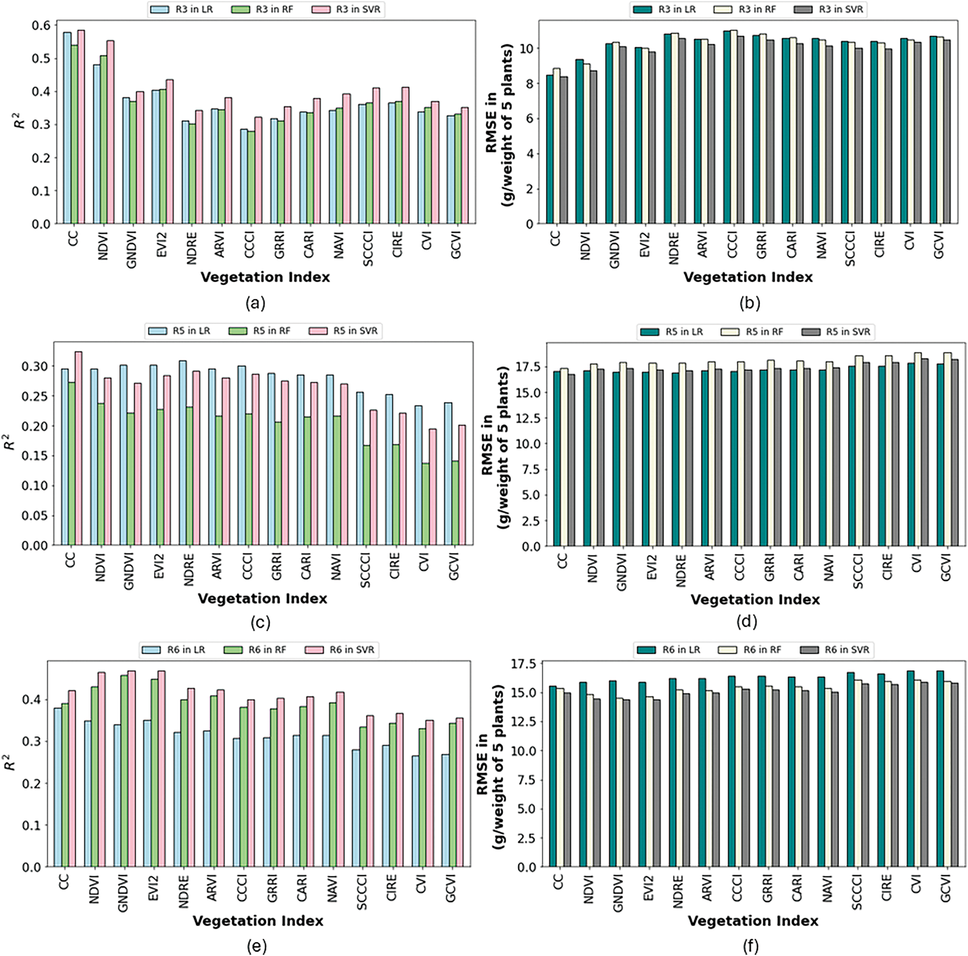
Figure 8: R2 values and RMSE values for R3 stage in (a,b), R5 in (c,d), and R6 (e,f), respectively, from biomass cross validated estimation modeling

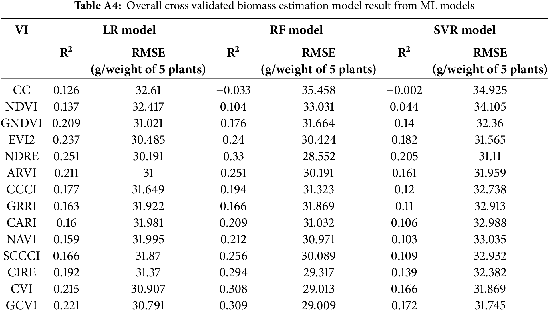
In addition, the total reproductive stages cross-validated modeling result is mentioned in Appendix A Table A4. We found the best estimation ability in cross-validated RF models, which had R2 about 0.1–0.31 and RMSE of 28–35 (g/weight of 5 plants). Similar results were observed in LR and SVR cross-validated models.

In LR models, we found that GNDVI, EVI2, NDRE, CVI and GCVI showed 0.20 to 0.25 estimation ability y whereas in SVR models, GNDVI, EVI2, NDRE, ARVI, CVI, and GCVI showed R2 about 0.14–0.21 estimation ability. Both models showed an RMSE range of about 31–35 (g/weight of 5 plants).

4  Discussion

With the development of modern agricultural systems, UAVs are widely applied in precision agriculture to monitor crop growth, bio-physical conditions, and yield. Soybean is a major crop in the United States and significantly contributes to the overall agricultural productivity. Application of UAV technology in soybean cultivation and management may reduce cost and labor and thereby contribute to the national economy.

It is reported that RS-based LAI estimation produces high errors during the crop reproductive stage due to canopy closure [10]. In this study, we precisely monitored soybean reproductive phases by estimating LAI and biomass. We developed ML approaches (i.e., LR, RF, SVR) to model LAI and biomass with VIs from UAV multispectral RS. Some researchers recommended that NDVI made LR model best suitable for LAI estimation [9]. We also found RF model is best suitable for LAI and biomass estimations compared to the LR and SVR models. LAI and biomass are complex, non-linear functions of spectral data, i.e., VIs. RF model can handle this complex non-linear relationship. It is an ensemble of decision trees, each trained on a random subset of data and features. This reduces variance and overfitting, leading to robust and accurate predictions, especially with noisy remote sensing data. RF model can work effectively without needing to eliminate correlated features or reduce dimensionality. RF can perform reasonably well even with small training datasets, unlike deep learning models. We also studied the changes of LAI and biomass during the growth season and reported the best phases to estimate these parameters from ML approaches.

Only a few studies monitored soybean growth phases by estimating plant biophysical parameters [9,42,43]. In this study, we have explored 14 VIs to determine the potential VIs for better growth estimates from the ML models. Some VIs, i.e., CC, NDVI, EVI2, ARVI, GRRI are mentionable for estimating these parameters for this studied crop. Others reported that NDVI and GNDVI are insensitive to crop type for LAI and biomass estimation [11].

We report that, for soybean crops, LAI is best estimated at R6 stage, whereas biomass is best estimated at R3 stage. Previous studies showed LAI was better estimatable at seed-filling (R5–R6) than at pod developing stage (R3–R4) [9]. In this study, we analyzed the sensitivity at each of the stages of LAI and Biomass, which is plotted in Figs. 6 and 7. We used R-2 (R-square) value to represent sensitivity. However, the cause of this different sensitivity could be because differences in spectral reflectance due to factors such as leaf chlorophyll content, leaf water content, and surface roughness can affect index values at different stages. Besides, Changes in the spectral properties due to senescence, disease, or stress can alter the relationship between the indices and actual LAI or biomass. The other factors could be canopying structure differences which include leaf angle distribution, canopy height, and density, influences how light interacts with vegetation. Different canopy structures can lead to variations in index values even if LAI or biomass remains constant. The other factors, like background impacts, the sensor types, and the climatic factors could also be responsible for this sensitivity difference.

One of the major impacts of this VI sensitivity variation can lead to reduced precision in LAI and biomass estimations, as changes in index values may not directly correlate with changes in these parameters. This also causes variability in estimations over time and space, complicating efforts to monitor and compare vegetation health and productivity across regions or seasons. High sensitivity to soil reflectance or atmospheric conditions can also lead to misinterpretation of vegetative index data, resulting in inaccurate assessments of plant health and productivity. Besides errors in the models used to predict LAI and biomass from vegetative indices can arise due to unaccounted variability, impacting the reliability of these predictions.

To mitigate VI sensitivity impacts, it is essential to develop more robust models that account for these sensitivities, use multi-spectral and hyperspectral data to improve accuracy, and employ advanced machine learning techniques to better understand and predict vegetation characteristics. Additionally, field validation and calibration remain crucial for ensuring the reliability of remote sensing-based estimations.

Overall, the results of this study will be helpful for monitoring soybean growth at reproductive phases which is a critical period for getting the most production. This research will aid the necessary information to national crop management.

5  Conclusion

This study monitored soybean reproductive phases using UAV-derived VIs to estimate LAI and biomass. These are major biophysical parameters for determining soybean growth conditions and productivity. We found the R6 stage is the best period for soybean LAI estimation, and the R3 stage for biomass estimation. The RF model outdated the LR and SVR model performance for the estimation of LAI and crop biomass. The leave-one-out cross-validation also strengthened the results. The use of VI index for estimating LAI and Biomass will reduce crop destruction and enhance production. The results of this study will be helpful for the proper management of soybean crops and production in farm fields, promoting improved agricultural crop management nationwide.

Acknowledgement: Not applicable.

Funding Statement: This research was supported in part by a postdoctoral research fellow appointment to the Agricultural Research Service (ARS) Research Participation Program administered by the Oak Ridge Institute for Science and Education (ORISE) through an interagency agreement between the U.S. Department of Energy (DOE) and the U.S. Department of Agriculture (USDA). ORISE is managed by Oak Ridge Associated Universities (ORAU) under DOE contract number DE-SC0014664. All opinions expressed in this paper are the author’s and do not necessarily reflect the policies and views of USDA, DOE, or ORAU/ORISE.

Author Contributions: Conceptualization: Sadia Alam Shammi and Yanbo Huang; methodology: Sadia Alam Shammi and Yanbo Huang; software, Weiwei Xie; validation: Sadia Alam Shammi, Yanbo Huang and Weiwei Xie; formal analysis: Sadia Alam Shammi and Weiwei Xie; investigation: Yanbo Huang; resources: Yanbo Huang; data curation: Weiwei Xie and Mark Shankle; writing—original draft preparation: Sadia Alam Shammi and Yanbo Huang; writing—review and editing: Sadia Alam Shammi, Yanbo Huang, Gary Feng, Haile Tewolde, Xin Zhang and Johnie Jenkins; visualization: Sadia Alam Shammi; supervision: Yanbo Huang; project administration: Yanbo Huang; funding acquisition: Yanbo Huang, Gary Feng, Haile Tewolde, Xin Zhang and Johnie Jenkins. All authors reviewed the results and approved the final version of the manuscript.

Availability of Data and Materials: The data presented in this article are publicly available in [usda-project-soybean-biomass-LAI] at [https://github.com/sadiashammi/usda-project-soybean-biomass-LAI (accessed on 24 August 2025)].

Ethics Approval: Not applicable.

Conflicts of Interest: The authors declare no conflicts of interest to report regarding the present study.

Appendix A

References

1. Dong T, Liu J, Qian B, He L, Liu J, Wang R, et al. Estimating crop biomass using leaf area index derived from Landsat 8 and Sentinel-2 data. ISPRS J Photogramm Remote Sens. 2020;168:236–50. doi:10.1016/j.isprsjprs.2020.08.003. [Google Scholar] [CrossRef]

2. Gong Y, Yang K, Lin Z, Fang S, Wu X, Zhu R, et al. Remote estimation of leaf area index (LAI) with unmanned aerial vehicle (UAV) imaging for different rice cultivars throughout the entire growing season. Plant Methods. 2021;17(1):88. doi:10.1186/s13007-021-00789-4. [Google Scholar] [CrossRef]

3. Qiao D, Yang J, Bai B, Li G, Wang J, Li Z, et al. Non-destructive monitoring of peanut leaf area index by combing uav spectral and textural characteristics. Remote Sens. 2024;16(12):2182. doi:10.3390/rs16122182. [Google Scholar] [CrossRef]

4. Tunca E, Köksal ES, Çetin S, Ekiz NM, Balde H. Yield and leaf area index estimations for sunflower plants using unmanned aerial vehicle images. Env Monit Assess. 2018;190(11):682. doi:10.1007/s10661-018-7064-x. [Google Scholar] [CrossRef]

5. Li H, Yan X, Su P, Su Y, Li J, Xu Z, et al. Estimation of winter wheat LAI based on color indices and texture features of RGB images taken by UAV. J Sci Food Agric. 2025;105(1):189–200. [Google Scholar]

6. Yamaguchi T, Tanaka Y, Imachi Y, Yamashita M, Katsura K. Feasibility of combining deep learning and RGB images obtained by unmanned aerial vehicle for leaf area index estimation in rice. Remote Sens. 2020;13(1):84. doi:10.3390/rs13010084. [Google Scholar] [CrossRef]

7. Liu S, Jin X, Nie C, Wang S, Yu X, Cheng M, et al. Estimating leaf area index using unmanned aerial vehicle data: shallow vs. deep machine learning algorithms. Plant Physiol. 2021;187(3):1551–76. doi:10.1093/plphys/kiab322. [Google Scholar] [CrossRef]

8. Du L, Yang H, Song X, Wei N, Yu C, Wang W, et al. Estimating leaf area index of maize using UAV-based digital imagery and machine learning methods. Sci Rep. 2022;12(1):15937. doi:10.1038/s41598-022-20299-0. [Google Scholar] [CrossRef]

9. Gao L, Yang G, Wang B, Yu H, Xu B, Feng H. Soybean leaf area index retrieval with UAV (unmanned aerial vehicle) remote sensing imagery. Chin J Eco-Agric. 2015;23(7):868–76. doi:10.13930/j.cnki.cjea.150018. [Google Scholar] [CrossRef]

10. Raj R, Walker JP, Pingale R, Nandan R, Naik B, Jagarlapudi A. Leaf area index estimation using top-of-canopy airborne RGB images. Int J Appl Earth Obs Geoinf. 2021;96(8–10):102282. doi:10.1016/j.jag.2020.102282. [Google Scholar] [CrossRef]

11. Kross A, McNairn H, Lapen D, Sunohara M, Champagne C. Assessment of RapidEye vegetation indices for estimation of leaf area index and biomass in corn and soybean crops. Int J Appl Earth Obs Geoinf. 2015;34:235–48. doi:10.1016/j.jag.2014.08.002. [Google Scholar] [CrossRef]

12. Maimaitijiang M, Sagan V, Sidike P, Maimaitiyiming M, Hartling S, Peterson KT, et al. Vegetation index weighted canopy volume model (CVMVI) for soybean biomass estimation from unmanned aerial system-based RGB imagery. ISPRS J Photogramm Remote Sens. 2019;151:27–41. doi:10.1016/j.isprsjprs.2019.03.003. [Google Scholar] [CrossRef]

13. Devia CA, Rojas JP, Petro E, Martinez C, Mondragon IF, Patiño D, et al. High-throughput biomass estimation in rice crops using UAV multispectral imagery. J Intell Robot Syst. 2019;96(3):573–89. doi:10.1007/s10846-019-01001-5. [Google Scholar] [CrossRef]

14. Bendig J, Yu K, Aasen H, Bolten A, Bennertz S, Broscheit J, et al. Combining UAV-based plant height from crop surface models, visible, and near infrared vegetation indices for biomass monitoring in barley. Int J Appl Earth Obs Geoinf. 2015;39:79–87. doi:10.1016/j.jag.2015.02.012. [Google Scholar] [CrossRef]

15. Shammi SA, Huang Y, Feng G, Tewolde H, Zhang X, Jenkins J, et al. Application of UAV multispectral imaging to monitor soybean growth with yield prediction through machine learning. Agronomy. 2024;14(4):672. doi:10.3390/agronomy14040672. [Google Scholar] [CrossRef]

16. Silleos NG, Alexandridis TK, Gitas IZ, Perakis K. Vegetation indices: advances made in biomass estimation and vegetation monitoring in the last 30 years. Geocarto Int. 2006;21(4):21–8. doi:10.1080/10106040608542399. [Google Scholar] [CrossRef]

17. Simic Milas A, Romanko M, Reil P, Abeysinghe T, Marambe A. The importance of leaf area index in mapping chlorophyll content of corn under different agricultural treatments using UAV images. Int J Remote Sens. 2018;39(15–16):5415–31. doi:10.1080/01431161.2018.1455244. [Google Scholar] [CrossRef]

18. Yang J, Xing M, Tan Q, Shang J, Song Y, Ni X, et al. Estimating effective leaf area index of winter wheat based on UAV point cloud data. Drones. 2023;7(5):299. doi:10.3390/drones7050299. [Google Scholar] [CrossRef]

19. Campos I, Gonzalez-Gomez L, Villodre J, Calera M, Campoy J, Jiménez N, et al. Mapping within-field variability in wheat yield and biomass using remote sensing vegetation indices. Precision Agric. 2019;20(2):214–36. doi:10.1007/s11119-018-9596-z. [Google Scholar] [CrossRef]

20. Bayaraa B, Hirano A, Purevtseren M, Vandansambuu B, Damdin B, Natsagdorj E. Applicability of different vegetation indices for pasture biomass estimation in the north-central region of Mongolia. Geocarto Int. 2022;37(25):7415–30. doi:10.1080/10106049.2021.1974956. [Google Scholar] [CrossRef]

21. Todd SW, Hoffer RM, Milchunas DG. Biomass estimation on grazed and ungrazed rangelands using spectral indices. Int J Remote Sens. 1998;19(3):427–38. doi:10.1080/014311698216071. [Google Scholar] [CrossRef]

22. Tilly N, Aasen H, Bareth G. Fusion of plant height and vegetation indices for the estimation of barley biomass. Remote Sens. 2015;7(9):11449–80. doi:10.3390/rs70911449. [Google Scholar] [CrossRef]

23. Mutanga O, Skidmore AK. Narrow band vegetation indices overcome the saturation problem in biomass estimation. Int J Remote Sens. 2004;25(19):3999–4014. doi:10.1080/01431160310001654923. [Google Scholar] [CrossRef]

24. Houborg R, McCabe MF. A hybrid training approach for leaf area index estimation via Cubist and random forests machine-learning. ISPRS J Photogramm Remote Sens. 2018;135:173–88. doi:10.1016/j.isprsjprs.2017.10.004. [Google Scholar] [CrossRef]

25. Zhang J, Cheng T, Guo W, Xu X, Qiao H, Xie Y, et al. Leaf area index estimation model for UAV image hyperspectral data based on wavelength variable selection and machine learning methods. Plant Methods. 2021;17(1):49. doi:10.1186/s13007-021-00750-5. [Google Scholar] [CrossRef]

26. Härkönen S, Lehtonen A, Manninen T, Tuominen S, Peltoniemi M. Estimating forest leaf area index using satellite images: comparison of k-NN based Landsat-NFI LAI with MODIS-RSR based LAI product for Finland. Boreal Environ Res. 2015;20(2):181–95. Available from: http://hdl.handle.net/10138/165218. [Google Scholar]

27. Zhang Y, Yang Y, Zhang Q, Duan R, Liu J, Qin Y, et al. Toward multi-stage phenotyping of soybean with multimodal UAV sensor data: a comparison of machine learning approaches for leaf area index estimation. Remote Sens. 2022;15(1):7. doi:10.3390/rs15010007. [Google Scholar] [CrossRef]

28. Zhu Y, Liu K, Liu L, Myint SW, Wang S, Liu H, et al. Exploring the potential of worldview-2 red-edge band-based vegetation indices for estimation of mangrove leaf area index with machine learning algorithms. Remote Sens. 2017;9(10):1060. doi:10.3390/rs9101060. [Google Scholar] [CrossRef]

29. Kang Y, Ozdogan M, Gao F, Anderson MC, White WA, Yang Y, et al. A data-driven approach to estimate leaf area index for Landsat images over the contiguous US. Remote Sens Environ. 2021;258:112383. doi:10.1016/j.rse.2021.112383. [Google Scholar] [CrossRef]

30. Geng L, Che T, Ma M, Tan J, Wang H. Corn biomass estimation by integrating remote sensing and long-term observation data based on machine learning techniques. Remote Sens. 2021;13(12):2352. doi:10.3390/rs13122352. [Google Scholar] [CrossRef]

31. Li KY, Sampaio de Lima R, Burnside NG, Vahtmäe E, Kutser T, Sepp K, et al. Toward automated machine learning-based hyperspectral image analysis in crop yield and biomass estimation. Remote Sens. 2022;14(5):1114. doi:10.3390/rs14051114. [Google Scholar] [CrossRef]

32. Sharma P, Leigh L, Chang J, Maimaitijiang M, Caffé M. Above-ground biomass estimation in oats using UAV remote sensing and machine learning. Sensors. 2022;22(2):601. doi:10.3390/s22020601. [Google Scholar] [CrossRef]

33. Han L, Yang G, Dai H, Xu B, Yang H, Feng H, et al. Modeling maize above-ground biomass based on machine learning approaches using UAV remote-sensing data. Plant Methods. 2019;15(1):10. doi:10.1186/s13007-019-0394-z. [Google Scholar] [CrossRef]

34. Reisi Gahrouei O, McNairn H, Hosseini M, Homayouni S. Estimation of crop biomass and leaf area index from multitemporal and multispectral imagery using machine learning approaches. Can J Remote Sens. 2020;46(1):84–99. doi:10.1080/07038992.2020.1740584. [Google Scholar] [CrossRef]

35. Mansaray LR, Kanu AS, Yang L, Huang J, Wang F. Evaluation of machine learning models for rice dry biomass estimation and mapping using quad-source optical imagery. GIScience Remote Sens. 2020;57(6):785–96. doi:10.1080/15481603.2020.1799546. [Google Scholar] [CrossRef]

36. Atkinson Amorim JG, Schreiber LV, de Souza MRQ, Negreiros M, Susin A, Bredemeier C, et al. Biomass estimation of spring wheat with machine learning methods using UAV-based multispectral imaging. Int J Remote Sens. 2022;43(13):4758–73. doi:10.1080/01431161.2022.2107882. [Google Scholar] [CrossRef]

37. Li B, Xu X, Zhang L, Han J, Bian C, Li G, et al. Above-ground biomass estimation and yield prediction in potato by using UAV-based RGB and hyperspectral imaging. ISPRS J Photogramm Remote Sens. 2020;162:161–72. doi:10.1016/j.isprsjprs.2020.02.013. [Google Scholar] [CrossRef]

38. Lao Z, Fu B, Wei Y, Deng T, He W, Yang Y, et al. Retrieval of chlorophyll content for vegetation communities under different inundation frequencies using UAV images and field measurements. Ecol Indic. 2024;158:111329. doi:10.1016/j.ecolind.2023.111329. [Google Scholar] [CrossRef]

39. Cawley GC. Leave-one-out cross-validation based model selection criteria for weighted LS-SVMs. In: Proceedings of the 2006 IEEE International Joint Conference on Neural Network Proceedings; 2006 Jul 16–21; Vancouver, BC, Canada. p. 1661–8. doi:10.1109/IJCNN.2006.246634. [Google Scholar] [CrossRef]

40. Gorriz JM, Segovia F, Ramirez J, Ortiz A, Suckling J. Is K-fold cross validation the best model selection method for Machine Learning? arXiv:2401.16407. 2024. doi:10.48550/arxiv.2401.16407. [Google Scholar] [CrossRef]

41. Fu B, Lao Z, Liang Y, Sun J, He X, Deng T, et al. Evaluating optically and non-optically active water quality and its response relationship to hydro-meteorology using multi-source data in Poyang Lake, China. Ecol Indic. 2022;145:109675. doi:10.1016/j.ecolind.2022.109675. [Google Scholar] [CrossRef]

42. Freitas Moreira F, de Oliveira HR, Lopez MA, Abughali BJ, Gomes G, Cherkauer KA, et al. High-Throughput phenotyping and random regression models reveal temporal genetic control of soybean biomass production. Front Plant Sci. 2021;12:715983. doi:10.3389/fpls.2021.715983. [Google Scholar] [CrossRef]

43. Da H, Li Y, Xu L, Wang S, Hu L, Hu Z, et al. Advancing soybean biomass estimation through multi-source UAV data fusion and machine learning algorithms. Smart Agric Technol. 2025;10:100778. doi:10.1016/j.atech.2025.100778. [Google Scholar] [CrossRef]