Numerical Approach to Simulate the Effect of Corrosion Damage on the Natural Frequency of Reinforced Concrete Structures

1  Introduction

RC1 structures are designed to be durable and to withstand environmental conditions while resisting different static and dynamic loads [1]. In theory, RC structures are designed to have a long service life expectancy, however, in practice premature failure of structures can occur due to underlooked responses or unforeseen events. It has been known for decades that a leading cause of premature structural failure in RC is corrosion [2]. The deterioration in the existing reinforced concrete (RC) structures, specifically in chloride-containing environments, has been also referred as corrosion and represents an ongoing global problem [3]. When corrosion propagates, steel area is reduced and rust is formed causing tensile stress to be generated at the interface between the reinforced steel bars and the concrete due to volume expansion. Bond strength is consequently affected when general corrosion arises [4].

The damage caused by corrosion in the reinforcement alters the functional and dynamical properties of the reinforced concrete structure, namely natural frequency and damping [5]. The effect of corrosion damage on dynamic properties has been investigated in different experimental programs. A special emphasis on vibration-based methods using dynamic parameters, i.e., natural frequencies, mode shapes, and vibration time-domain responses is noticed in many attempts [6]. However, the effect of corrosion damage on damping is to be controversial with inconsistent trends recorded in different studies [7]. Therefore, this study considers only the relationship between natural frequency and corrosion damage.

Several structural problems are known to be magnified by corrosion attack altering the structural performance and the nonlinear response [8]. Therefore, quantifying the relationship between natural frequency and corrosion is essential to mitigate premature failure [9]. In addition, this relationship is considered attractive in non-destructive structural health monitoring settings where there have been multiple research attempts dealing with vibration-based structural damage detection [10]. Yet, many constraints arise in this field. They are mainly attributed to the limited available data, the complex nature of corrosion, and the involvement of multidisciplinary fields.

Many attempts have shed light on the powerfulness of using dynamic behavior alteration as a way to detect damage in structures. In their study, Zhang et al. [11] asserted that when the dynamic response of bridge structures is measured from vibration tests, it could be employed in the assessment of the structural health and safety conditions. Surprisingly, this technique has been revealed since early last decade when Mazurek et al. [12] assumed that the deterioration level of a structure is quantifiable using vibrational analysis.

Marc et al. [13] added that an enhanced opportunity to detect damage in reinforced concrete structures lies in the nonlinear dynamic signs. Mode shape changes and frequency response functions are studied and compared to be employed in damage detection [14]. Accordingly, Quy et al. pioneered an experimental study [15], on the minaret (24.25 m high) of Hacılar mosque where the dynamic system characteristics variation served as the leading mean to detect the cracks and their locations. Owolabi et al. [14] were among the first scientists to deal with frequency variation as a damage detector in reinforced concrete beams. In their study, they quantified the variations in the first three natural frequencies and their corresponding amplitudes in an attempt to present a damage detection scheme for RC beams.

Based on what is mentioned above, corrosion in steel bars is shown to cause perturbations in the structural integration of Reinforced Concrete (RC) elements. In terms of the mechanical properties, a clear and certain distraction of the load-deflection behavior is spotted. Such differences induce a modification in the dynamical behavior of the aforementioned elements too. As a result, the seismic behavior of RC elements and buildings is interrupted when corrosion enters the game.

The revealed alterations in the structural parameters are of high importance and should be regarded carefully as they influence the safety of occupants and users of the structure.

In this study, a numerical attempt to simulate the effect of corrosion damage on the variation of the natural frequency of the structure is presented. The approach relies on simulating the time history response of the structure using a modified Bouc-Wen model that incorporates the nonlinear effects of corrosion. Then, a modal analysis is utilized to assess the change in natural frequency [16]. Lastly, machine learning regression algorithms in MATLAB® (Regression Learner App) are employed to find the optimal relationship between input structural properties, including corrosion damage, and natural frequency. The presented framework is illustrated using thirteen RC multistory buildings. All the buildings are made of a cantilevered-column lateral resisting system and each building is subjected to seven different levels of corrosion. The results derived denote a promising quantitative relationship between corrosion damage and natural frequency variation of multistory building with cantilevered column lateral resisting system. They also serve as a reference for future investigations of other types of lateral resisting RC systems.

2  Numerical Modeling

A full numerical framework for simulating the behavior of corroded reinforced concrete buildings is presented in this study. The suggested approach relies on simulating the dynamic time history response of the corroded building, under dynamic loads, based on the Bouc-wen algorithm [17] and by modifying it to incorporate the effect of corrosion damage. Then, the response at different corrosion levels is fed into output-only model analysis algorithms to extract the variation in the natural frequency of the structure [18]. Finally, machine learning tools are employed to derive a quantitative relationship between natural frequency, corrosion damage and various structural parameters. For this study, the corrosion level represents the loss in cross-sectional area of steel bars. It is worth mentioning that the computer code for the numerical simulation was written on MATLAB ® version R2018a. OoMA toolbox and machine learning toolbox in MATLAB ® were utilized for output-only modal analysis and for regression analysis, respectively, as detailed in this section.

2.1 Time History Analysis

2.1.1 Hysteretic Model

Structures under dynamic loads are subjected to hysteretic behavior. However, under repeated cyclic loadings, there are continuous deformations and deterioration of the reinforced concrete structures [19]. Limited hysterical models are capable of accurately representing the deteriorating and non-linear hysteretic behavior of RC structures. This study employs the Bouc-wen model for this task as it has proven successful performance in different studies, [1] and [20] as examples. This model is known for its versatility and mathematical tractability which has made it popular in different engineering problems, including multi-degree of freedom systems [21]. It has also been utilized to analyze seismic excitation and dynamic response, to forecast the health of an RC structure, and to estimate the nonlinear behavior of the structure under low and high excitation, which is the case in this study. Moreover, Bouc-wen has gained experimental and numerical validation through the years.

The Bouc-wen model is a modification of the well-known equation of motion (Eq. (1)) that adds several control parameters to capture the non-linear hysterical performance of the system, as described below:

The equation of motion is:

My¨+Cy˙+RT=F(t) (1)

where M is the system mass, C is the damping,  RT is the system nonlinear restoring force, the over dots in  y(t)  variables show the derivatives with respect to time, then y¨ and  y˙ represent acceleration and velocity respectively and F(t) is the applied force. Moreover, this equation of motion is developed to correspond to model and the restoring force is expressed as:

RT=αkiy(t)+(1−α)kiz(t) (2)

where αkiy(t) represents the linear component, while (1−α)kiz(t)   is the hysteretic component; ki is the elastic stiffness of the system, α is the stiffness ratio and z(t) is the hysteretic displacement, which is differentiated to become:

z˙(t)=Ay˙(t)−(β|y˙||z(t)|n−1 z(t)+γy˙(t)|z(t)|n)  (3)

with the initial conditions z(0)=0 . The parameters  A. α.β.γ and n  control the shape of hysteresis loops.

The equation of motion according to the Bouc-Wen model is expressed:

My¨+Cy˙(t)+αKy(t)+(1−α)Kz(t)=−Mu¨g(t)  (4)

where u¨g represents the ground acceleration.

In the adopted numerical setup, the Runge Kutta integration is utilized to determine the system time history response. This integration method is most suitable for simulating long-term transformations for dynamical models governed by higher ordinary differential equations [22].

2.1.2 Alteration of Structural Properties

The corrosion mechanism is one of the main reasons for the alteration in structural properties. There are two different phenomena of corrosion: General corrosion in steel bars is uniform or localized corrosion that leads to pitting corrosion [23]. Once corrosion initiates along the reinforced steel bar, pitting corrosion occurs in localized sites. According to [24], the crucially pitting corrosion phenomenon induces local stress concentrations which highly impacts the fatigue life of structures. As the maximum pitting depth is considerably higher than uniform penetration, the ratio between pitting and uniform corrosion depths is taken as a mean value 5.65 to estimate the maximum pitting depth  p(t) [25].

After estimating the maximum pitting depth, the remaining area of the steel bar diameter is calculated as follows:

Dremaining= D0−p(t) (5)

%Alost= (1−Dremaining2D02)×100  (6)

where D0 is the initial bar diameter in mm, Dremaining is the bar diameter at any time t , p(t) is the pit depth from Eq. (2) and Alost  is the relative loss of area in percentages.

Eqs. (5) and (6) simulate the reduction in the cross-sectional of steel affecting the cracking and effective moments of inertia. Consequently, the stiffness (K) of the building, which is a main parameter in the elastic and inelastic behavior of the Bouc-wen model, is updated according to the different corrosion levels.

In this study, the proposed model in [26] is adopted. This model has been similarly approached in more recent studies, [27] and [28]. Thus, the prediction curve depicted in Eqs. (7) and (8) is believed to be representative of the actual bond strength behavior at different corrosion levels. It denotes the actual bond strength behavior, in which corrosion up to 2% depicts an increase in bond strength and decreases beyond 2% [26].

ub=16.87    for C0≤2.0 (7)

ub=24.7 C0−0.55  for C0>2.0 (8)

where ub is the bond strength,  C0 is the corrosion level in %.

2.1.3 Effect of Slippage

Slippage in the reinforcing bars exhibits a significant magnification under corrosion effects. This leads to reduced bond strength and therefore additional lateral deformation in the system due to rotational drift,  θs . The deformation of slippage may be as large as the flexural deformation [29] and is calculated as follows [30]:

θs=εsfsdb8ub(d−c)  for εs ≤ εy  (9)

where db is the tensile steel bar diameter, c is the depth of the neutral axis, fs is the stress in steel bars, εs is the actual strain of the tensile reinforcement at the column joint level,  εy being the yield strain of steel and d is the depth to tensile reinforcement from the top.

2.1.4 Total Drift

The Bouc-wen model, with the updated stiffness, is now utilized to determine the total time history displacement at each time step incorporating the effect of corrosion damage on the structural response [9]. This approach relies on modifying the initial Bouc-Wen parameters to account for the reduction in steel bars and the effect of slippage at each floor as per the equation below [31].

Consequently, the strain and stress at each floor level can be determined. Then the rotational slippage is computed according to the computed stress at each story level and the updated bond strength using Eq. (9). Δ2 is then computed using Eq. (11) and the total displacement is simulated by summing Δ1 and Δ2 according to Eq. (10).

Δtotal = Δ1 + Δ2 (10)

Δ2=θs×h  (11)

where Δtotal is the total drift resulting from the modified Bouc-Wen model, Δ1 is the drift value caused by the dynamic loads with updated parameters due to mass loss (elastic and inelastic stiffness), and Δ2 is the additional drift initiated by slippage.

2.2 Modal Analysis

Modal analysis establishes the dynamic properties of structural systems in the frequency domain which represents the analysis of mathematical functions or signals with respect to their frequency instead of time. It is known that a time-domain graph describes how a signal changes over time, whereas a frequency-domain the graph illustrates the number of signals lying within each given frequency band over a series of frequencies [7].

For this aim, two major mathematical programming processes are employed to detect the modal parameters of the structure: Input-Output Modal Analysis and Output-Only Modal Analysis.

An ideal modal analysis incorporates controlling and measuring the excitation to the system. However, in large-scale civil structures, such as buildings, it is not pertinent to apply controllable excitation to conduct the classical input–output modal test. This is also revealed in the measurement of the ambient excitation that may be caused by wind and earthquakes. For this reason, output-only identification methods are favorable in practice especially when only structural responses are available [32].

For this study, where total displacement values are accessible, the output-only modal analysis tool, namely Stochastic Subspace Identification (SSI), is used in the next stage.

2.2.1 Stochastic Subspace Identification (SSI )

The data-driven from the Stochastic Subspace Identification is looked at as the most effective tool among the other known identification techniques in the time domain. The input parametric model is matched to the raw times series data where its parameters are adjusted to change the way the model fits the data. The aim is to minimize the deviation between the predicted system response of the model and the measured system response (measurements) known as calibration. Overschee et al. [33] were the first to initiate the stochastic subspace identification algorithm (Data-SSI). Robust numerical techniques are implemented to identify the state space matrices such as QR-factorization, SVD2 and least squares. Being employed in several types of civil engineering structures, the SSI is considered as one of the strongest and most accurate system identifications in output only [34].

2.2.2 Machine Learning

Finding an algorithm that simulates the change of natural frequency with corrosion damage is useful in different fields, like data assimilation and health monitoring. As an example, a simple non-destructive measure of the natural frequency of a built structural element could lead to the detection of the level of corrosion inside its reinforcement. In addition, it is a computationally efficient approach that simplifies the complicated and multidisciplinary process of simulating modal behavior under corrosion damage. Though, involving all the above-described methods does not lead to a straightforward relationship between corrosion and variation of dynamic properties, however, the suggested numerical scheme can be utilized as a cheap alternative, to experimental programs, to export reliable data. Here comes the need to introduce a machine learning process, or regression learner, to deal with a large amount of data and variables present in this study. Therefore, combining the numerical approach that simulates dynamic response and a regression learner scheme, leads to an optimal numerical relation between corrosion damage and modal parameters for different structural configuration.

3  Numerical Application

To illustrate the suggested numerical framework, thirteen different building configurations, shown in Table 1, are utilized. Each building is investigated at eight different levels of corrosion damage: 0, 1.75, 3.5, 7.5, 10, 12.5, 17.5, and 22.5%. The common assumptions employed for modeling of these buildings are listed below:

1.    Cantilevered columns structural system: cantilevered column elements only for lateral resistance.

2.    Identical flat slabs, 15 cm thickness, with no beams in any direction.

3.    Concrete 28-day compressive strength, f’c = 35 MPa.

4.    Grade 60 reinforcing bars with yielding strength, fy = 413.7 MPa.

5.    All vertical elements are subjected to the same level of corrosion damage.

6.    Total mass contribution in the dynamic analysis at each floor is 95000 kg.

Three only parameters have been modified in each building case: the number of floors, the section of the columns, and the reinforcement ratio, ρ .

ρ=100×AsAg  (12)

where As represents the total reinforcement area in the column and Ag is the cross-section area of the column.

A uniform plan setup displayed in Fig. 1 is considered in each building, where 4 and 3 columns are placed in the X and Y directions, respectively. The center-to-center span length between each column equals five meters.

Figure 1: Plan view of the building

3.1 Lateral Load: Pulse

In the simulations, a pulse signal excitation at the top of the building is performed to initiate the dynamic response. In signal processing, a pulse has an amplitude that changes rapidly and momently from a baseline value to a higher or lower value succeeded by a direct return to the baseline value [35]. The characteristics of the pulse signal aid in identifying the frequency content of the system under the simulated various corrosion rates.

3.2 Numerical Results

3.2.1 Lateral Displacement

The total lateral displacement of the corroded RC buildings is obtained using the modified Bouc-Wen procedure. At each mode, the displacement values are derived before being processed using the SSI3. To illustrate the buildings’ total displacement, the response of a pulse excitation of building B8, at 0% and 12.5% corrosion levels is shown in Fig. 2. It is quite clear in both curves that there is a jump to reach maximum displacement after initial excitation, and then the displacement fades to zero due to the damping effect. The effect of corrosion damage is evident in the curve with 12.5% corrosion level, where the displacement has a higher peak and a higher period of oscillation (lower frequency) as compared to the uncorroded displacement response.

Figure 2: Total displacement in function of time spotted at two different corrosion levels for the same building under pulse excitation

3.2.2 Natural Frequency

The natural frequency is detected using Stochastic Subspace Identification. The displacement values derived using the Bouc-Wen procedure are treated for the first three modes of the three floors buildings, B1, B2, and B3 and for the first five modes for B3, B4, B5, B6, B7, B8, B9, B10, B11, B12, and B13. In each building case, under different corrosion levels, the natural frequency values are derived for each mode, by creating a stabilization diagram using the functions in the OoMA toolbox in MATLAB® to aid in the selection of stable poles and model order. The adopted stabilization criteria are 2% error in frequency, 5% error in damping and 98% confidence in mode shape vectors. The corrosion level 0 represents the control state of the building where no theoretical corrosion has been induced yet. The thirteen buildings are designated as BNx where N represents the number of the building, and x the theoretical corrosion level in percentage. For illustration, a sample of the results is presented in Fig. 3 for the 8th building.

Figure 3: Average Natural Frequencies detected at different corrosion levels for Building 8

For B80%, an increase in the natural frequency is remarked at each mode increment. It departs from 1.833 Hz at mode 1 and reaches 27.105 Hz at mode 5. Similar behavior of the natural frequency value is shown for each corrosion rate of the considered building. The finding above, derived from modified Bouc-Wen simulation and Modal analysis, can be linked to the basic formulation of the natural frequency equation which proportionally relates the mode number to the natural frequency.

fn=12n2πEImL4 

where fn is natural frequency, n is the mode number, E is the modulus of elasticity, I is the second moment of area, M is the mass per unit length and L is the span length.

It was noted that the drop in frequency is consistent among all the modes. For example, the frequency of all modes dropped by nearly 1.6% and 8.3% in B83.5% and B817.5%, respectively, from their initial value at the uncorroded state. This is reflected in Fig. 3 where the trend line of mode 5 shows a continuing decrease as the corrosion level increases.

Next, the change in frequency is documented in percentage (%), as the remaining frequency, in comparison to the initial frequency of the uncorroded state. For simplicity, the results of the first three modes are only presented in Table 2, and the results of mode 1 of all buildings in shown in Fig. 4 since a similar behavior of drop in frequency is remarked among all modes.

Figure 4: Frequency variation (%) with respect to the Corrosion level (%) at the first mode of each building under excitation load

In Fig. 4, the corrosion level is shown to affect the natural frequency for each of the considered building cases. A common variation trend is observed among all buildings, where the natural frequency variation increases with the increase of the corrosion level at all modes.

On the other hand, the results indicate that the impact of corrosion on the drop in frequency is altered by several parameters. Back to Table 2, buildings are grouped as G1, G2, G3, and G4 where each group has the same number of floors and column sections, namely stiffness, while only the steel ratio ρ is varied between the 3 building cases of each group (1%, 2% and 4%). This allows for further insight into the effect of ρ . It is worth noting that buildings B9 and B13 do not belong to any group since they have different floor numbers and/or column sections, thus they do not match the grouping criteria employed in this section. Their main purpose is to generalize and randomize the training data and the validation.

It is evident from Fig. 5 that the effect of corrosion is magnified as the steel ratio increases, resulting in a higher frequency variation at similar levels of corrosion. For example, in group G1, buildings are composed of 3 floors, and the columns’ section is 45 × 45 cm. When the columns reinforcement ratio, ρ , is set to be 1%, the natural frequency drops by 3.19% when 22.5% corrosion rate is applied in mode 3. However, the frequency variation is higher at 5.59% and 9.32% for the same corrosion level and mode number in buildings B2 and B3 respectively. This is also revealed in G2, G3, and G4, where a higher reinforcement ratio leads to a higher frequency variation when corrosion attacks the building.

Figure 5: Frequency variation of group G1 buildings at each corrosion level for the first three modes

Another finding can be spotted when investigating the effect of the remaining input variables. Although less significant, the dimensions of the building’s structural elements appear to impact the results. For example, buildings B4 and B7 have the same input variable with only variation in the columns section, however, the drop in frequency is slightly more revealed in the building where larger column sections exist. The average variation in frequency is higher by 6% in building B7 in comparison to building B4 at different corrosion levels, as expressed in Fig. 6.

Figure 6: Frequency variation vs. corrosion level (%) for buildings B4 and B7

The effect of column size can be also confirmed when comparing B9 with B12, where the building with a larger column section, B12, witnessed a higher frequency drop at all corrosion levels. The same conclusion can be drawn when comparing B6 with B8, the drop in frequency is consistently more significant in stiffer buildings for all levels of corrosion.

3.3 Regression Analysis and Machine Learning

The interpretation of the adopted numerical approach leads to consistent outcomes. This shed the light on the possibility of deriving a correlation between the different involved parameters that can be used as a cheaper and more practical alternative for full numerical modeling. For this aim, many classical and advanced statistical methods can be used. Using the analysis of results found in the previous section, three input parameters were selected as predictors for drop in frequency, dF (in %), expected when corrosion attacks the building. The parameters are column dimension h (in cm), steel ratio in columns ρ (in %), and the corrosion level in columns, CL (in %). It is confirmed afterward using p-values in regression analysis, that all these parameters are significant to simulate the drop in frequency.

In this study, the extracted data is processed with two different methods: First, using the simplest known regression technique, the Multivariate Linear Regression Analysis (MLRA), and then using the best fitting model in the machine learning toolbox in MATLAB®, known as the regression learner APP. 25% of data are not used in the model training process and are left out for model validation.

3.3.1 Multivariate Linear Regression Analysis (MLRA)

The widely used multivariate regression analysis is employed to merge all the results derived from the above-explained procedures. MLRA is noticeably similar to the simple linear regression model. Yet, it deals with multiple independent variables contributing to the dependent variable.

Based on an MLRA4, an equation to describe the statistical relationship between one or more predictor variables and the response variable is generated:

dF=−3.55+0.0161 h+1.032 ρ+0.341 CL  (14)

The R square value of the regression model was found to be 0.89, which means that 89% of the predicted values fit the regression analysis model. In other words, 89% of the dependent variables are explained by the independent variables ( h,ρ, and CL ) along with the assigned coefficients. Moreover, the p-value for all coefficients was found to be below 0.05, indicating that all these parameters can be assumed correlated to the drop in frequency. Although, these regression parameters, the R-square and the p-values, make this approach sound promising, when investigating the predicted response vs. the actual data, as presented in Fig. 3, anomalies of the MLRA model can be captured.

The 45° line in Fig. 7a serves as the reference line between the true response (simulated data) and the predicted response from the trained linear model. It is obvious from both graphs, (a) and (b), that the model is biased and is not providing proper prediction along the range of the response. This assures that multi-variate linear regression is not the best-fit model with an evident non-linear residual trend as shown in the graph and a high percentage of predicted error reaching up to 600%.

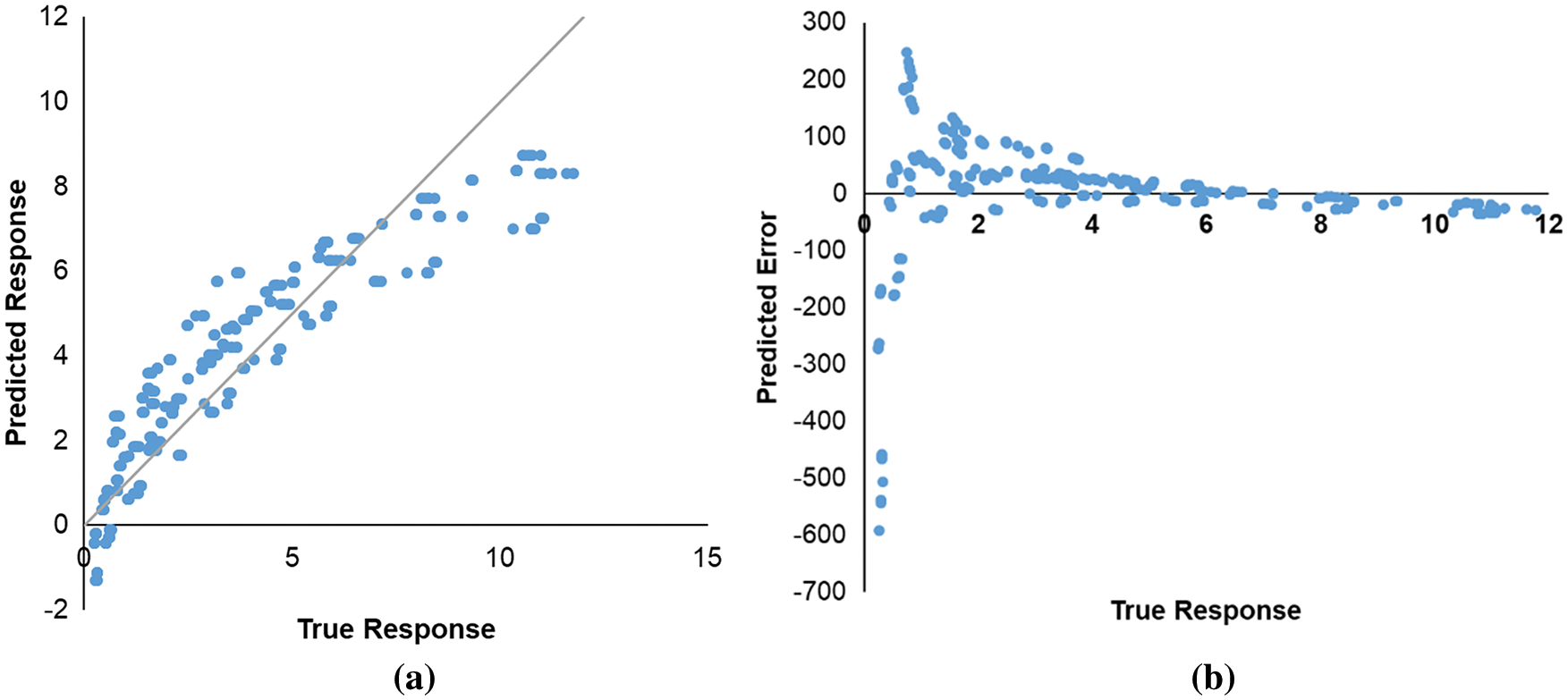
Figure 7: (a) True response vs. predicted response derived using MLRA (b) True Response vs. percentage error derived using MLRA

3.3.2 Machine Learning Tool: Squared Exponential Gaussian Process Regression (GPR)

The results derived from the MLRA showed discrepancies when compared to the actual simulated data. This led to the use of a more advanced statistical analysis approach, by relying on a powerful existing machine learning tool, the regression learner app in MATLAB®. This tool trains 22 models, on linear and non-linear analyses basis, for the available data. The best-fit model can be selected based on the minimum root mean square error (RMSE), as shown in Table 3.

Using this approach on the simulated data, the SE-GPR5 was nominated as the optimal model with a RMSE equals 0.106. The GPR6 is a nonparametric, Bayesian approach to regression that is showing success in the area of machine learning. One of the GPR several benefits is working well on small datasets, which is the case in this study. The Gaussian process aims to calculate the probability distribution over all admissible functions that fit the data. The GPR works by specifying a prior (on the function space), calculating the posterior using the training data, and computing the predictive posterior distribution on the points of interest. Various covariance functions can be incorporated with GPR to completely define the process’ behavior, such as linear, constant, white Gauss noise, squared exponential, periodic, etc. [36].

The input data that has been used in the regression learner app, is based on the proper output data of the previous phases of this study, and is the same as the one used in the multivariate linear regression analysis. The predicted dF values used to calibrate the regression models are found using the displacement records collected from the modified Bou-wen methodology. The corresponding natural frequencies, and the estimated drop accordingly, are next estimated by the mean of output-only modal analysis at different modes. Once introduced in the Regression Learner App, very close values of dF to the exact values simulated by the numerical models are observed.

Moreover, the SE-GPR model yields significantly less error when compared to the MLRA has an RMSE error of 0.965.

Further investigation of the SE-GPR was performed by plotting the actual data vs. the predicted response and percentage error from True response as shown in Fig. 8. This graph can be utilized to assess the model performance. The plot assures the power of the selected model as an optimal fit. Discrepancies are significantly reduced between actual drops in frequency and the predicted ones, where the points appear to be very close to the 45° line in Fig. 8a. It is also worth noting that the residuals do not reflect any evident bias or pattern and a maximum error of 15% is observed in the graph of Fig. 8b.

Figure 8: (a) True response vs. predicted response derived using SE-GPR (b) True response vs. percentage error derived using SE-GPR

For additional assessment and validation of the trained models, numerical samples and percent errors of the left-out data are presented in Table 3 below. The graphical representation of the matching between the predicted drop in the frequency and the actual drop in frequency of showed in for all left-out data is presented in Fig. 9. The average absolute error of the 25% left-out data was found to be around 2% and 80% using the SE-GPR and MLRA models, respectively. It can be once again concluded from Tables 3, 4 and Fig. 9 that the SE-GPR approach has a clear advantage over the use of the classical multivariate linear regression analysis to find the drop in frequency when the corrosion rate, steel reinforcement ratio, and columns dimensions of the building are known. These regression results confirm that the SE-GPR in this case, or simulated-data-driven machine learning can act as an efficient alternative to predict the drop in the natural frequency of buildings due to corrosion damage. It is worth mentioning again that the study’s tests were limited to thirteen buildings with square cantilevered columns, however, this study opens the door to utilizing the same approach for more general and complicated structures.

Figure 9: Predicted error in natural frequency response for the left-out data using SE-GPR and MLRA regression learner tools

3.4 Model Verification

Validating simulation models is a complex and difficult task in the current general setup. The difficulty depends on benchmarking against real-time experimental measurements and the few attempts to correlate the variability of dynamic properties with corrosion damage. However, this has become possible by using various numerical and experimental measurements listed below:

•   First, the initial state of the uncorroded structure is examined by matching the outcomes of the nonlinear behavior of the structure to a typical dynamic analysis of the same structure in ETABS®. Both modeling techniques are compared for their maximum internal drift showing a good agreement with a maximum variance of 12%.

•   Next, this study uses the experimentally validated approach in other papers, [37–39], to simulate the effect of steel loss and slippage under seismic loadings so that the effect of corrosion damage is well depicted.

•   Furthermore, the overall dynamic performance of the proposed approach was compared with the experimental program of four double-bent columns presented in [40]. In the current research attempt, using a modified Bouc-Wen approach, the impact of the slip deformation is estimated to be between 23%–35% of the total displacement for various building configurations. This conclusion matches the findings of the experimental investigation elaborated in [40] stating that the slippage contribution ranges from 25% to 40% of the total lateral displacement as depicted in Fig. 10. It is noted that the percentage contribution of displacement is defined as 100 times the ratio of the respective deformation quantity to the total displacement at the same time in Fig. 10.

•   Lastly, the current study proposes a relationship between corrosion damage and change in natural frequency using the output-only modal analysis. In this study, an average of 2.43% frequency drop is expected for an approximately 7.5% corrosion level as can be noted in Table 2. This does not contradict the results of the experimental program in [7]. Abdul Razak and Choi investigated the frequency drop in two corroded beams (D1 and D3) with nearly 8% corrosion level, where the average drop among all modes was found to be around 6.3% and 2% as depicted in Table 5 [7].

Figure 10: Contribution of displacement components to total lateral displacement [40]

4  Conclusion

This study develops a full numerical scheme to predict the drop in the natural frequency of multi-story buildings at different corrosion levels. The scheme relies on a modified Bouc-Wen algorithm that simulates the lateral displacement under a pulse excitation. Furthermore, an output-only analysis approach, the SSI, is employed to detect the natural frequency in the structure. The cheap nature of the numerical scheme is attractive to simulate sufficient data that can be used in calibrating efficient regression algorithms.

Generally, the numerical results presented herein show that corrosion of reinforcement in the tested buildings caused significant changes to the modal parameter, namely natural frequency and this converges with many research attempts, as in [41]. It’s worth mentioning that the simulated drop in frequency in this study is as well with a close range with the experimental findings of Abdul Razak et al. [7] at similar corrosion damage.

The results have been interpreted in a way to find a relationship between the different parameters involved in the study. Using classical and more advanced linear regression techniques has shown that a relationship exists between the different factors. The SE-GPR application, which is used in machine learning, is a promising tool for detecting the drop of natural frequency in corroded structures when further studies are conducted.

It is finally worth emphasizing that the SE-GPR function derived in this study is only limited to structures that have a braced column-like behavior, however, a similar analogy can be applied for different types of lateral resisting systems.

In conclusion, the use of numerical modeling in the way enlightened in this study could present a reliable alternative for simulating the effect of corrosion damage on the dynamic properties of reinforced concrete structures.

Funding Statement: This work is part of the research project entitled: “A Sustainable Structural Health-Monitoring Framework for Service-life Prediction of Corroded RC Structures Using Induced Vibration-Response Analysis” conducted by A. El Kordi, W. Slika, R. Machmouci, and A. Hakim. The authors received joint funding for this project from the National Council for Scientific Research-Lebanon (CNRS-L) and the Beirut Arab University. Research Project (12-05-2018).

Conflicts of Interest: The authors declare that they have no conflicts of interest to report regarding the present study.

1Reinforced Concrete.

2Singular Value Decomposition.

3Stochastic Subspace Identification.

4Multivariate Linear Regression Analysis.

5Squared Exponential Gaussian Process Regression.

6Gaussian Process Regression.

References

1. Slika, W., Saad, G. (2018). Probabilistic identification of chloride ingress in reinforced concrete structures: Polynomial chaos kalman filter approach with experimental verification. Journal of Engineering Mechanics, 144(6). https://doi.org/10.1061/(ASCE)EM.1943-7889.0001463 [Google Scholar] [CrossRef]

2. Ma, Y., Guo, Z., Wang, L., Zhang, J. (2020). Probabilistic life prediction for reinforced concrete structures subjected to seasonal corrosion-fatigue damage. Structural Engineering, 146(7), 305. https://doi.org/10.1061/(ASCE)ST.1943-541X.0002666 [Google Scholar] [CrossRef]

3. Zhang, M. Y., Akiyama, M., Shintani, M., Xin, J. Y., Frangopol, D. M. (2021). Probabilistic estimation of flexural loading capacity of existing RC structures based on observational corrosion-induced crack width distribution using machine learning. Structural Safety, 91. [Google Scholar]

4. Michele, W. T. M., Pieter, D., Janet, M. L. (2019). Corrosion-induced cracking and bond strength in reinforced concrete. Construction and Building Materials, 208(3), 228–241. https://doi.org/10.1016/j.conbuildmat.2019.02.151 [Google Scholar] [CrossRef]

5. Lee, H. S., Cho, Y. S. (2009). Evaluation of the mechanical properties of steel reinforcement embedded in concrete specimen as a function of the degree of reinforcement corrosion. International Journal of Fracture, 157(1–2), 81–88. https://doi.org/10.1007/s10704-009-9334-7 [Google Scholar] [CrossRef]

6. Zhenghao, D., Jun, L., Hong, H. (2022). Simultaneous identification of structural damage and nonlinear hysteresis parameters by an evolutionary algorithm-based artificial neural network. International Journal of Non-Linear Mechanics, 142. [Google Scholar]

7. Abdul Razak, H., Choi, F. C. (2001). The effect of corrosion on the natural frequency and modal damping of reinforced concrete beams. Engineering Structures, 23(9), 1126–1133. [Google Scholar]

8. Zhang, M., Liu, R., Li, Y., Zhao, G. (2018). Seismic performance of a corroded reinforce concrete frame structure using pushover method. Advances in Civil Engineering, 1(1), 1–12. https://doi.org/10.1155/2018/7208031 [Google Scholar] [CrossRef]

9. Mashmoushy, R. (2021). Reliability analysis of reinforced concrete structures subjected to chloride induced corrosion under seismic loading (Master’s Thesis). Beirut Arab University, Beirut. [Google Scholar]

10. Chunwei, Z., Asma, A. M., Sami, F. M., Gholamreza, G., Kai, Y. et al. (2022). Vibration feature extraction using signal processing techniques for structural health monitoring: A review. Mechanical Systems and Signal Processing, 177, 109175. https://doi.org/10.1016/j.ymssp.2022.109175 [Google Scholar] [CrossRef]

11. Nguyen, T. Q. (2022). Damage detection in beam structures using bayesian deep learning and balancing composite motion optimization. Structures, 39(1), 98–114. https://doi.org/10.1016/j.istruc.2022.03.030 [Google Scholar] [CrossRef]

12. Mazurek, D. F., Dewolf, J. T. (1990). Experimental study of bridge monitoring technique. Journal of Structural Engineering-American Socity of Civil Engineers, 116, 2532–2549. [Google Scholar]

13. Marc, R., Rafik, H., Nazih, M. (2014). Nonlinear structural damage detection based on cascade of Hammerstein models. Mechanical Systems and Signal Processing, 48(1–2), 247–259. https://doi.org/10.1016/j.ymssp.2014.03.009 [Google Scholar] [CrossRef]

14. Owolabi, G. M., Swamidas, A. S. J., Seshadri, R. (2003). Crack detection in beams using changes in frequencies and amplitudes of frequency response functions. Journal of Sound Vibration, 265(1), 1–22. https://doi.org/10.1016/S0022-460X(02)01264-6 [Google Scholar] [CrossRef]

15. Quy, T. N., Ramazan, L. (2022). A health monitoring solution on damage detection of minarets. Engineering Failure Analysis, 135. [Google Scholar]

16. Chiplunkar, A., Morlier, J. (2017). Operational modal analysis in frequency domain using gaussian mixture models. In: Topics in modal analysis & testing, pp. 47–53. Cham: Springer. [Google Scholar]

17. Goda, K., Hong, H. P., Lee, C. S. (2009). Probabilistic characteristics of seismic ductility demand of SDOF systems with Bouc-Wen hysteretic behavior. Journal of Earthquake Engineering, 13(5), 600–622. https://doi.org/10.1080/13632460802645098 [Google Scholar] [CrossRef]

18. Mashmoushy, R., Slika, W., Elkordi, A. (2021). A novel probabilistic framework of RC corroded structures under dynamic loading. BAU Journal-Science and Technology, 2(2). [Google Scholar]

19. Ikhouane, F., Rodellar, J. (2007). Systems with hysteresis analysis, identification and control using the Bouc-Wen model. England: John Wiley and Sons. [Google Scholar]

20. Ismail, M., Ikhouane, F., Rodellar, J. (2009). The hysteresis Bouc-Wen model, a survey. Archives of Computational Methods in Engineering, 16(2), 161–188. https://doi.org/10.1007/s11831-009-9031-8 [Google Scholar] [CrossRef]

21. Masri, S. F., Caffrey, J. P., Caughey, T. K., Smyth, A. W., Chassiakos, A. G. (2004). Identifcation of the state equation in complex non-linear systems. International Journal of Non-Linear Mechanics, 39(7), 1111–1127. https://doi.org/10.1016/S0020-7462(03)00109-4 [Google Scholar] [CrossRef]

22. Cash, J. R., Karp, A. H. (1990). A variable order Runge-Kutta method for initial value problems. ACM Transactions on Mathematical Software, 16(3), 201–222. https://doi.org/10.1145/79505.79507 [Google Scholar] [CrossRef]

23. Abou Shakra, J., Joumblat, R., Khatib, J., Elkordi, A. (2020). Corrosion of coated and uncoated steel reinforcement in concrete reinforcement in concrete. Beirut Arab Univeristy Journal-Science and Technology, 2(1). [Google Scholar]

24. Sulaiman, S., Peter, S., Tim, B. (2022). Probabilistic modelling of pitting corrosion and its impact on stress concentrations in steel structures in the offshore wind energy. Marine Structures, 84. [Google Scholar]

25. Di Maio, F., Fumagalli, M., Guerini, C., Perotti, F., Zio, E. (2021). Time-dependent reliability analysis of the reactor building of a nuclear power plant for accounting of its aging and degradation. Reliability Engineering & System Safety, 205(8), 107173. [Google Scholar]

26. Chung, L., Kim, J. J., Yi, S. T (2008). Bond strength prediction for reinforced concrete members with highly corroded reinforcing bars. Cement & Concrete Composites, 30(7), 603–611. https://doi.org/10.1016/j.cemconcomp.2008.03.006 [Google Scholar] [CrossRef]

27. Liu, M., Jin, L., Chen, F., Zhang, R., Du, X. (2022). 3D meso-scale modelling of the bonding failure between corroded ribbed steel bar and concrete. Engineering Structures, 256(8), 113939. https://doi.org/10.1016/j.engstruct.2022.113939 [Google Scholar] [CrossRef]

28. Sun-Jin, H., Hyunjin, J., Deuckhang, L. (2022). Practical approach for estimating flexural strengths of corroded RC members considering bond strength degradation. Structures, 39(1), 808–820. https://doi.org/10.1016/j.istruc.2022.03.072 [Google Scholar] [CrossRef]

29. Sezen, H., Setzler, E. J. (2008). Reinforcement slip in reinforced concrete columns. American Concrete Institute Structural Journal, 105(3), 280–289. [Google Scholar]

30. Siamphukdee, K., Collins, F., Zou, R. (2019). Sensitivity analysis of corrosion rate prediction models utilized for reinforced concrete affected by chloride. Journal of Materials Engineering and Performance, 22(6), 1530–1540. [Google Scholar]

31. Inci, P., Goksu, C., Ilki, A., Kumbasar, N. (2013). Effects of reinforcement corrosion on the performance of RC frame buildings subjected to seismic actions. Facilities, 27(6). [Google Scholar]

32. Ayisha, N., Ummul, B., Muhammad, A., Syed, A. Z. N., Asif, I. (2022). Damage detection based on output-only measurements using cepstrum analysis and a baseline-free frequency response function curvature method. Science Progress, 105(1). https://doi.org/10.1177/00368504211064487 [Google Scholar] [CrossRef]

33. Overschee, P. V., Bart, D. M. (1993). Subspace algorithms for the stochastic identification problem. Automatica, 29(3), 649–660. https://doi.org/10.1016/0005-1098(93)90061-W [Google Scholar] [CrossRef]

34. Brincker, R., Andersen, P. (2006). Understanding stochastic subspace identification. IMAC-XXIV : A Conference & Exposition on Structural Dynamics, Society for Experimental Mechanics, St. Louis, Missouri, USA. [Google Scholar]

35. Molina, A., González, J. (2016). Pulse voltammetry in physical electrochemistry and electroanalysis. USA: Springer. [Google Scholar]

36. Rasmussen, C. E., Williams, C. K. (2006). Gaussian processes for machine learning. USA: The MIT Press. [Google Scholar]

37. Bichara, L., Saad, G., Slika, W. (2019). Probabilistic identification of the corrosion propagation rate in reinforced concrete structures via deflection and crack width measurements. Construction and Building Materials, 52, 52–89. [Google Scholar]

38. Vu, N. S., Yu, B., Li, B. (2016). Prediction of strength and drift capacity of corroded reinforced concrete columns. Construction and Building Materials, 115, 304–318. https://doi.org/10.1016/j.conbuildmat.2016.04.048 [Google Scholar] [CrossRef]

39. Molaioni, F., di Carlo, F., Rinaldi, Z. (2021). Modelling strategies for the numerical simulation of the behaviour of corroded RC columns under cyclic loads. Applied Sciences, 11(20), 9761. https://doi.org/10.3390/app11209761 [Google Scholar] [CrossRef]

40. Halil, S., Jack, P. M. (2006). Seismic tests of concrete columns with light transverse reinfrocement. ACI Structural Journal, 103(6), 842–849. [Google Scholar]

41. Jarek, A., Dos Santos, A. T., Bragança, M. O. G. P., Pinkoski, I. M., Neri, M. A. T. et al. (2022). Experimental and numerical investigations to evaluate the structural integrity of concrete beams exposed to an aggressive coastal environment. Structures, 37, 795–806. https://doi.org/10.1016/j.istruc.2022.01.059 [Google Scholar] [CrossRef]