Paradigm of Numerical Simulation of Spatial Wind Field for Disaster Prevention of Transmission Tower Lines

1  Introduction

With the development of the electric power industry, more attention has been paid to electric power safety. As an indispensable part of power system operation, the reliability and stability of the transmission process is one of the current hot issues discussed. With the continuous expansion of the erection range of high-voltage overhead transmission lines, the erection area is gradually expanded to locations with more complex geographical environments and harsh climatic conditions, and the requirements for transmission line protection are steadily increased.

The regional environmental factors for the erection of transmission tower lines are complex and often extreme climates, so the transmission tower lines are prone to wind disasters during operation. The transmission tower line structure itself has the characteristics of the tower height, large span, and sizeable overall structure flexibility [1]. It is easy to be corrupted by extreme weather conditions, so that line breaking and collapse accidents occur, resulting in transmission line operation and maintenance faults, which seriously threaten the safety and stability of the transmission process.

Under the action of strong wind, transmission tower line collapse, line breaking, and other accidents happen from time to time, seriously endangering the transmission process’s safety and stability. Fig. 1 shows a power transmission tower collapse accident in one place. It also causes great economic losses to the power system. On June 14, 2005, a 500 kV power transmission line in Siyang, Jiangsu Province suffered a severe squall disaster, resulting in a wind-caused tower toppling accident. This accident caused the tripping of the temporary line and stopped transmission of the two lines simultaneously, leading to huge losses to East China Power Grid [2]. In Xiamen, Fujian Province, due to the landfall of Typhoon Morandi 1614, several substations of the Xiamen power grid and hundreds of power transmission lines of different grades lost power. It left 522,000 customers without power, and five power transmission towers in mountainous areas collapsed [3].

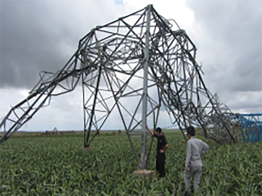
Figure 1: A power transmission tower collapsed due to strong wind

In previous wind field studies, wind speed is usually assumed to be a stationary stochastic process. However, a large amount of measured data shows that the actual wind field of strong wind mainly presents non-stationary characteristics, and the mean wind speed changes with time. Tao et al. compared stationary and non-stationary wind fields and proposed an adaptive method to automatically extract time-varying mean values to characterize non-stationary wind [4]. Hao et al. analyzed typhoon fields in stationary and non-stationary models and realized the simulation of non-stationary typhoon fields using a multi-variable method [5].

In the simulation analysis of the wind-induced dynamic response of transmission lines, the fluctuating wind speed is usually regarded as a sequence with a mean value of 0 and conforming to normal distribution. While ignoring the effect of high-order parameters of wind speed, the unique spatial correlation between fluctuating wind speed series at different locations is not considered. Wind speed generally presents Gaussian characteristics when it is less disturbed by terrain. But in particular environments such as mountains or valleys, wind speed is easily affected by local terrain, which presents significant non-Gaussian characteristics. Duan conducted wind tunnel tests on three-dimensional steep slope type and canyon and discussed the influence of these two notable landforms on the essential characteristics of fluctuating wind [6]. Gao coupled the typhoon field with the special mountain terrain, proving that the basic characteristics of the wind field would change under the action of micro-terrain [1].

The numerical simulation of the response of the transmission tower line under the action of strong wind can effectively study the wind-induced response law of the transmission tower line. Moreover, simulation can be used to explore the wind resistance of transmission tower line structures and forecast the possibility of wind disasters.

To simulate and analyze the wind response of the transmission tower line structure, it is necessary to obtain the input wind load time series. The time series of wind loads can be obtained through field measurement, wind tunnel tests, or numerical simulation. The numerical simulation method is often used in wind loads simulation analysis because of its convenience, speed, repeatability, and regularity advantages.

The wind-vibration response of transmission tower lines has been a hot topic in recent years. Considering that the wind speed at each point of the model is not entirely independent, the temporal and spatial correlation should be taken into account in the calculation. By analyzing the measured wind speed data, Duan obtained the influencing factors of the spatial correlation of wind speed and the variation rules [6]. Yan et al. introduced the Fourier phase difference spectrum to establish the correlation calculation model [7]. Lorenzo et al. simulated the mechanical response of tower structures by simulating the time history of hurricane wind speed against the background of the collapse of tower lines in Cuba [8]. Zhang gave the calculation flow of simulating single-point and multi-point Gaussian and non-Gaussian wind speed time history [9]. Zhang et al. gave the calculation flow of non-Gaussian fluctuating wind simulation for transmission tower lines by using the linear filter method [10]. Shen et al. compared the simulation results of fluctuating wind speed under different methods and used cross-spectrum to simulate a three-dimensional wind field [11].

Regarding non-Gaussian wind simulation, Chang compared various conversion methods and concluded that the correlation function conversion method was more intuitive and straightforward than the spectral updating method [12]. Kim et al. adopted the K-L extension method and iterative translation approximation method to simulate non-stationary non-Gaussian stochastic processes, which can improve the simulation accuracy and computational efficiency [13]. Wen extended the simulation method of frequency wave number spectrum (FKS) based on SRM to the simulation of non-Gaussian random waves, which ensured the compatibility of FKS and edge probability density function (PDF) and improved the iteration efficiency [14]. Jiang improved the traditional Johnson change method with linear prediction and the Z transform (LZP) method. In the spectral updating method, he proposed a CDF mapping algorithm based on linear prediction and Z transform (LZP) to simulate non-Gaussian wind pressure [15].

The above studies are perfect for wind load simulation of transmission tower line systems but are less involved in non-Gaussian wind field simulation. Most of the research focuses on the effect of fluctuating wind on structure, but the overall impact of the wind field is not explored. This paper proposes a simulation method of non-Gaussian fluctuating wind based on previous studies. Considering the characteristics of the actual wind field, the numerical simulation of the overall spatial wind field is carried out, which provides a research basis for the wind-induced response simulation of transmission tower lines.

2  Review of Research Status

2.1 Wind Speed Simulation Method

Space wind can be generally regarded as two parts: mean wind and fluctuating wind. Mean wind refers to the long-period part whose vibration period is over 10 min. In contrast, fluctuating wind refers to the short-period part whose vibration period is between a few seconds and tens of seconds. The Monte Carlo method is used for the numerical simulation of fluctuating wind. The principle of the Monte Carlo method is to use a random simulation method for sampling and calculating the value of statistics or parameters. In the case of a large number of calculations, the average value of each calculation result is obtained to get a stable value, and a conclusion is drawn. The methods of simulating wind fields by the Monte Carlo method generally include the harmonic superposition and linear filter methods.

The linear filter method is also known as the autoregressive method. Its working principle is to input a group of random white noise numbers with a zero mean into a designed filter for transformations and output wind speed time series with the specified wind speed spectral density characteristics. The linear filter method was first proposed in 1987 by Iannuzzi et al. [16]. Owen et al. compared the simulation results of wind speed time history with the AR method and ARMA method and believed that the simulation accuracy of the ARMA method was relatively high [17]. Peng et al. gave the linear filter method simulation steps and the model order determination method [18]. Li et al. combined the Fourier transform with the linear filter method to broaden the application range of the linear filter method [19].

The linear filter method has advantages because of its small computation amount and fast computation speed. This paper adopts a linear filter AR autoregressive model to simulate the fluctuating wind numerically and verify whether the generated results meet the preset requirements.

2.2 Non-Gaussian Wind Simulation

Generally, fluctuating wind is regarded as a stationary Gaussian process in numerical simulation. However, fluctuating wind presents strong non-Gaussian characteristics in the complex terrain environment where transmission tower lines are erected. Because of its special distribution law, non-Gaussian wind is easy to cause damage to the tower lines. Therefore, it is necessary to conduct a numerical simulation of non-Gaussian wind to explore the response results of its action on the transmission tower lines.

To explore the influence of stationary non-Gaussian fluctuating wind on the numerical analysis of the wind-induced response of actual transmission tower lines, the Gaussian wind simulation results must be converted to the non-Gaussian wind by the static conversion method. There are two kinds of conversion methods for simulating non-Gaussian processes.

The first method is based on the given power spectral density function and edge distribution probability function. This method requires updating and iterating the power spectral density function to obtain a non-Gaussian random process.

The second method is based on the given power spectral density function and high-order moments such as skewness and kurtosis. In this method, the relation between the Gaussian and non-Gaussian processes is obtained by converting the correlation function. Gurley first proposed to transform non-Gaussian operations based on Hermite polynomials. Grigoriu gave the basic idea and calculation process of transformation through correlation function, which does not require multiple iterative calculations [20]. Gioffre et al. extended the calculation scope to the field of multi-variables and discussed the simulation method and fitting coefficient of non-Gaussian wind pressure [21].

Recently, many improved methods have been proposed for correlation function transformation. Wu et al. considered the fractal characteristics of non-Gaussian wind, combined with the correlation deformation method and simulated non-Gaussian wind [22]. Zhang established a novel non-Gaussian stochastic process simulation transformation method based on the generalized lambda distribution of FMKL [23]. Considering the standard deviation of the random process, Luo et al. gave the calculation formula of inverse function conversion from a non-Gaussian correlation function to a Gaussian correlation function [24]. According to the transformation relation of the non-Gaussian process, Cai gave the calculation formula of the transformation parameter [25].

The above method summarizes a relatively convenient and rapid simulation method, but only the numerical simulation of non-Gaussian fluctuating wind is carried out. The influence of the overall instantaneous wind speed simulation on calculating the spatial correlation function is not explored, and the corresponding research on the transmission tower line still needs to be improved.

3  Numerical Simulation Method of Spatial Wind Field

The instantaneous value of spatial wind can be regarded as consisting of average wind and fluctuating wind, namely:

v(x, y, z, t)=v¯(x, y, z, t)+vf(x, y, z, t) (1)

In the process of numerical simulation, it is necessary to simulate the mean wind and fluctuating wind respectively, and overlay the results.

3.1 Numerical Simulation of Mean Wind

The variation of average wind speed with height is called wind profile. Commonly used wind profiles include logarithmic wind profiles and exponential wind profiles, whose expressions are given as follows [26]:

v¯z1=1kv¯∗ln(z1z0) (2)

v¯z1v¯z2=(z1z2)α (3)

In formula (2), k is the von Karman coefficient, and k takes 0.4; z1 and z0 are the effective height and the height of the rough ground layer, respectively; v∗ and v¯z1 are the atmospheric shear velocity and the average wind speed at z1 altitude, respectively. In formula (3), z1 and z2 are the height of two points, respectively; v¯z1 and v¯z2 are the average wind speed at two points, respectively; α is the surface roughness coefficient.

The calculation of logarithmic wind profile is more complicated, which is suitable for calculating the average wind speed below 100 m. This paper uses the exponential law wind profile to calculate the average wind speed. The roughness is selected as B type according to the national load standard, and the surface roughness coefficient is α=0.16 .

3.2 Power Spectrum for Fluctuating Wind Simulation

Fluctuating wind can be divided into turbulent airflow in three directions: downwind, sideways, and vertical. The transverse and vertical winds have low turbulence intensity and have little effect on the wind-induced response of the transmission tower line structure [26]. Generally, their effect can be ignored in the research, and the wind-induced response of the transmission tower line under downwind turbulence is analyzed.

The fluctuating wind can be regarded as a stationary random process with a mean value of 0, which can be analyzed mainly through the power spectral density function. The power spectral density function represents the energy distribution of fluctuating wind speed in the frequency domain. Based on the combination of theory and experiment, the approximate distribution function, namely the power spectral density function, can be obtained through the statistics and fitting of the test data. Davenport calculated according to the measured data and believed that the turbulence scale of the horizontal fluctuating wind velocity spectrum did not change with the height. The empirical expression of Davenport’s fluctuating wind velocity spectrum was summarized as follows:

nSv(n)v¯102=4Kx2(1+x2)43 (4)

where x=1200n/v¯10 ; SV(n) is power spectral density; k is the surface roughness coefficient; n=ω/2π is the frequency of fluctuating wind; v¯ 10 is the average wind speed at a standard altitude (the altitude is usually 10 m).

3.3 Spatial Correlation of Fluctuating Wind Simulation

The wind speed blown to each location is not completely independent in the actual environment. Due to the influence of other areas, the wind speed and direction of fluctuating wind at each point are only partially synchronized. This property is called spatial correlation. The spatial correlation is related to the distance. The greater the distance between two points, the smaller the spatial correlation.

The spatial correlation function can quantify spatial correlation. Fluctuating wind’s downwind mutual power spectral density can represent its statistical characteristics. The spatial correlation function is the ratio of the amplitude of the mutual power spectral density at two points to the amplitude of the self-power spectral density function:

coh(f)=|S12(f)|S11(f)S22(f) (5)

where S11(f) and S22(f) are self-power spectral density at two points, respectively; S12(f) is cross-power spectral density.

The spatial correlation function has a variety of expressions. This paper uses the exponential expression form proposed by Davenport. The following expression is usually used in wind engineering to express the coherence of the vertical direction of fluctuating wind [27]:

coh(f)=exp{−n[cz2(zi−zj)2]12[V¯(zi)+V¯(zj)]} (6)

where v¯(zi) and v¯(zj) are the wind speed at points i and j, respectively; cz are attenuation coefficients in the z-direction. Generally, cz takes 10.

3.4 Gaussian Fluctuating Wind Simulation Method

In this paper, the linear filter AR method is used to simulate Gaussian wind speed. The specific steps are as follows:

The time series formula of stationary Gaussian wind speed for M spatially correlated points is [28]:

u(X, Y, Z, t)=−∑k=1p⁡Ψk⋅u(X, Y, Z, t−kΔt)+N(t) (7)

where u(X, Y, Z, t) is the stationary Gaussian fluctuating wind speed (m/s) at multiple points in space; p is the autoregressive order of the AR model; X=[x1, …, xM]T , Y=[y1, …, yM]T , Z=[z1, …, zM]T are space point coordinates, respectively; N(t)=L⋅n(t) , where n(t) is M independent standard normally distributed random time series, and L is a/the coefficient matrix.

To get the coefficient matrix Ψk , multiply u(t−jΔt) on both sides of the equation, and calculate the expectation. The autocorrelation function expression on the stationary Gaussian wind speed time history can be obtained as follows:

R(jΔt)=−∑k=1p⁡ΨkR[(j−k)Δt] (8)

R(0)=−∑k=1p⁡ΨkR[kΔt]+RN (9)

Express formula (9) in matrix form to get the following equation [9]:

R⋅Ψ=[RNOp] (10)

where Ψ=[I, Ψ1, …, ΨP]T is the autoregressive parameter matrix of the AR model of order (p+1)M×M , and every submatrix is a square matrix of order M. Op is a zero matrix of order pM×M ; RN is a square matrix of order M.

The submatrix of R can be obtained by the Wiener–Khintchine formula [9]:

Rij(τ)=∫0∞⁡Sij(f)cos(2πf⋅τ)df (11)

where Sij is the cross-power spectrum, which can be calculated by the self-power spectrum and spatial correlation function [28]:

Sij(f)=coh(f)⋅Sii(f)Sjj(f) (12)

After the Cholesky decomposition of RN , the coefficient matrix L can be obtained. After the normal distribution random sequence is generated, the time series of the Gaussian process fluctuating wind speed can be obtained by substituting L into formula (7).

The AIC criterion is used to determine the order p of the AR model, and the model can meet the requirements of practicality and complexity when the minimum AIC function is selected. Given the upper limit of order N, the AIC criterion of the AR model is defined as [18]:

AIC(p)=N∗lgσ^∂2+2(p+1) (13)

where σ∂2=2R(0)−R(N) .

From AR(1) to AR(p + 1), a total of p + 1 AIC models are established, and the AIC criterion function values of each model are compared, respectively. When the function difference between AR(p) and AR(p + 1) is minimal, the order p can be selected [18]. In this simulation method, the value of p is 4.

Therefore, the simulation flow of the program for calculating non-Gaussian fluctuating wind time series u(t) is as follows:

1)   The wind speed self-power spectrum specified in the program is the Davenport wind speed spectrum. The expression Sij of the cross-power spectral density function between every two points is obtained by using the spatial correlation formula.

2)   The matrix values of the cross-correlation function Rij(0) to Rij(pΔt) between two points are obtained by using the Wiener–Khintchine formula, respectively. Then R is established.

3)   The parametric matrix Ψ is obtained from p⋅M equations after the system. Then the matrix RN is obtained from the first M equations.

4)   The Cholesky decomposition of RN yields the coefficient matrix L.

5)   M groups of independent standard normal distribution random time series n(t) are generated, and N(t)=L⋅n(t) is calculated.

6)   The time series u(t) of multi-point Gaussian wind velocity is obtained by substituting L into formula (7).

3.5 Non-Gaussian Fluctuating Wind Simulation Conversion Method

Gaussian fluctuating wind loads can be described using mean and variance. The mean value represents the oscillation center of the random wind signal, and the variance represents the dispersion degree of the signal amplitude relative to the mean value. The high-order cumulant of the time series of stationary non-Gaussian wind loads is not zero, so it is necessary to introduce high-order parameters, such as skewness coefficient and kurtosis coefficient, in the simulation of non-Gaussian fluctuating wind.

Skewness represents the degree of deviation of signal amplitude from the oscillating center. The skewness of the Gaussian process is 0 by default. Non-Gaussian processes become positive skewness when their skewness is positive. The reverse is called negative skewness, and the diagram is shown below. Kurtosis indicates how sharp or flat a curve is, and the kurtosis of a Gaussian process defaults to 3. When the kurtosis of the non-Gaussian process is greater than 3, the curve is sharper, and the tail is longer, which is called the soft response process. When the curve is less than 3, the curve is flatter, and the tail is shorter, called the hard response process [29].

In this paper, the correlation deformation method proposed by Gurley is used to simulate non-Gaussian wind time series. The principle is to convert the Gaussian time series simulated by the linear filter method into a non-Gaussian time series by correlation formula given the high-order moments. The formula is as follows:

Rx=α2(Ru+2h32Ru2+6h42Ru3) (14)

x(t)=α[u(t)+h3(u(t)2−1)+h4(u(t)3−3u(t))] (15)

where u(t) and Ru are Gaussian fluctuating wind speed sequence and its autocorrelation function, respectively; x(t) and Rx are non-Gaussian fluctuating wind speed sequence and autocorrelation function, respectively.

The relevant parameters α , h3 and h4 can be obtained by solving the above nonlinear equations, and can also be approximated according to the given high-order moments: skewness γ3 and kurtosis γ4 [30]. They can be calculated according to the following formula derived from the empirical model [25]:

α=11+2h32+6h42 (16)

h3=γ36[1−0.015|γ3|+0.3γ321+0.2(γ4−3)](17)

h4=h40[1−1.43γ32γ4−3]1−0.1(γ4)0.8 (18)

h40=[1+1.25(γ4−3)]13−110 (19)

The variance σ2 of Davenport fluctuating wind speed spectrum is calculated as follows:

σ2=∫0∞⁡S(f)df=12.4289 (20)

After considering the standard deviation, the expression of the conversion equation is modified as follows:

x(t)σ=α{u(t)+h3{[u(t)]2−1}+h4{[u(t)]3−u(t)}} (21)

Rxij(τ)=α2σ2{Ruij(τ)+2h32[ Ruij(τ)]2+6h42[Ruij(τ)]3} (22)

Solving the inverse function of the conversion function can obtain the expression of the Gaussian process [24]:

Ruij=1α(G1−G1G2−h329h42) (23)

G1=118h42−h3481h44 (24)

G2=[Rxijσ212h42+(Rxij/σ212h42+G3)2+G13+G3]1/3 (25)

G3=h32108h44−h36729h46 (26)

The parameters h3 and h4 need to satisfy the following relation to make the conversion equation valid [25]:

h32−3h4(1−3h4)≤0 (27)

The conditions to be met for γ3 and γ4 can be obtained by using the formula [25]:

3+(1.25γ3)2≤γ4 (28)

3.6 Non-Gaussian Fluctuating Wind Simulation Method

By combining the Gaussian fluctuating wind speed simulation method introduced in Section 3.4 above with the non-Gaussian fluctuating wind speed simulation conversion method presented in Section 3.5 above, a complete non-Gaussian fluctuating wind speed simulation method can be obtained, and its process is shown in Fig. 2.

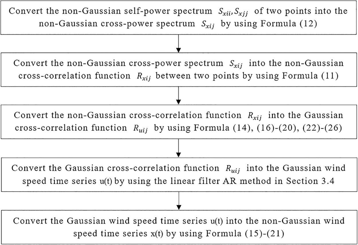
Figure 2: Flowchart of non-Gaussian fluctuating wind simulation method

In this simulation method, the standard deviation of the wind speed spectrum is added to the traditional conversion equation, and the conversion equation is modified. Luo et al.’s method [24] is introduced into the calculation of Gaussian and non-Gaussian process conversion methods, which reduces the complexity of calculating the inverse function formula (14). Meanwhile, the relationship between the calculation parameters h3 and h4 and the set wind speed skewness and kurtosis γ3 and γ4 is clarified [25]. The non-Gaussian wind speed simulation method is improved and synthesized, and the complete method flow is introduced in detail in this paper.

4  Examples and Results of Spatial Wind Simulation

4.1 Example and Parameter Setting

To verify the feasibility of the fluctuating wind generation method in numerical simulation of the wind-induced response of actual transmission tower lines, a transmission tower is selected to simulate non-Gaussian wind field generation. The transmission tower is located in a mountainous area. The topography has a significant influence on the wind speed change, and the transmission tower is prone to strong wind vibration response at different heights, which will cause harm to its stability.

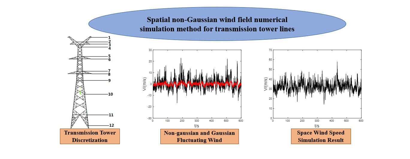
The height of the transmission tower line is more than 40 m, and the wind speed is not the same at different heights. Theoretically, every node of the transmission tower will bear a particular wind load when the strong wind is flowing, so it is the closest method to the actual condition to accurately simulate the global wind speed field and apply it to the transmission tower. In fact, due to the limitations of computer storage capacity and calculation speed, it is not possible or necessary to simulate the wind speed of every node in the transmission tower. Therefore, the finite element method is used to discretize the transmission tower, and the average height of each section is selected to simulate the wind field of the transmission tower. Before wind-induced response simulation, the transmission tower is first discretized and divided into 12 sections from top to bottom, which is shown in Fig. 3. The average wind speed at the average height of each section is taken as the average wind speed of the section.

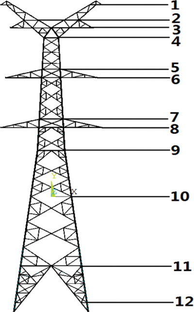
Figure 3: Schematic diagram of transmission tower discretization

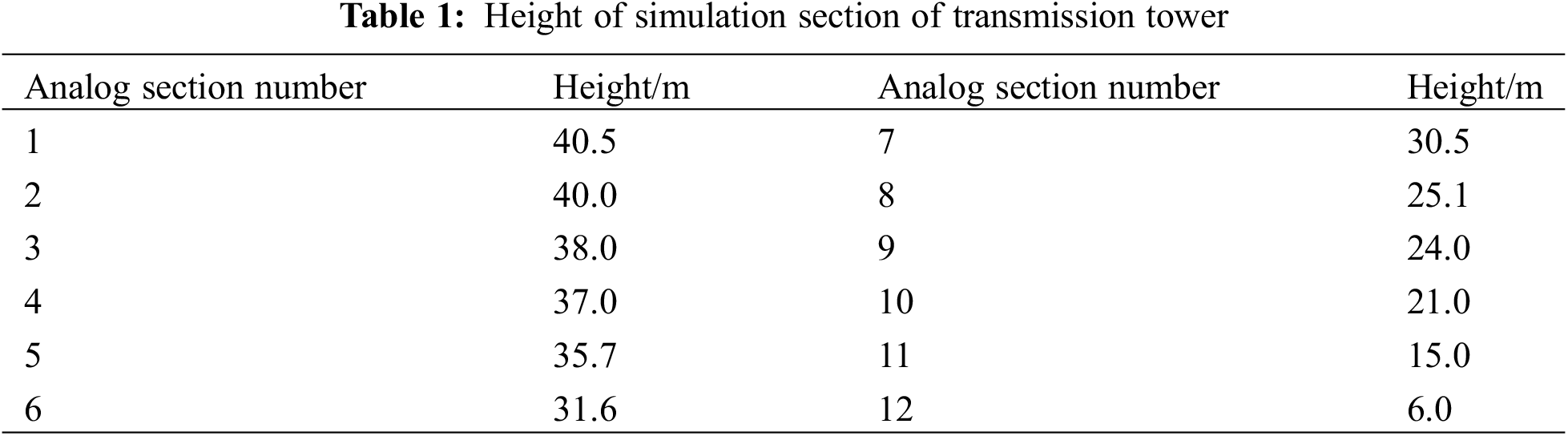
The height of each simulation section after discretization is shown in Table 1.

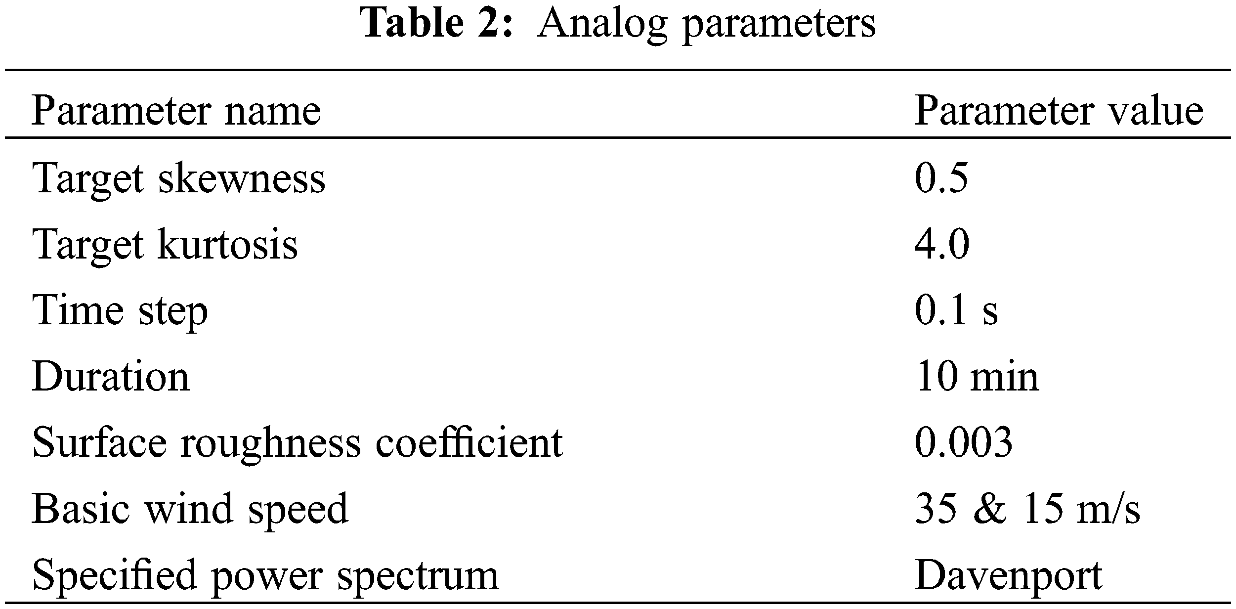
The parameters used in the simulation are in Table 2.

4.2 Simulation Results and Verification

Based on the following parameters, wind field simulation was carried out according to the method summarized in the paper. A total of 20 groups were simulated and skewness and kurtosis at 12 sectional heights were calculated. The average value of the results is shown in Tables 3 and 4.

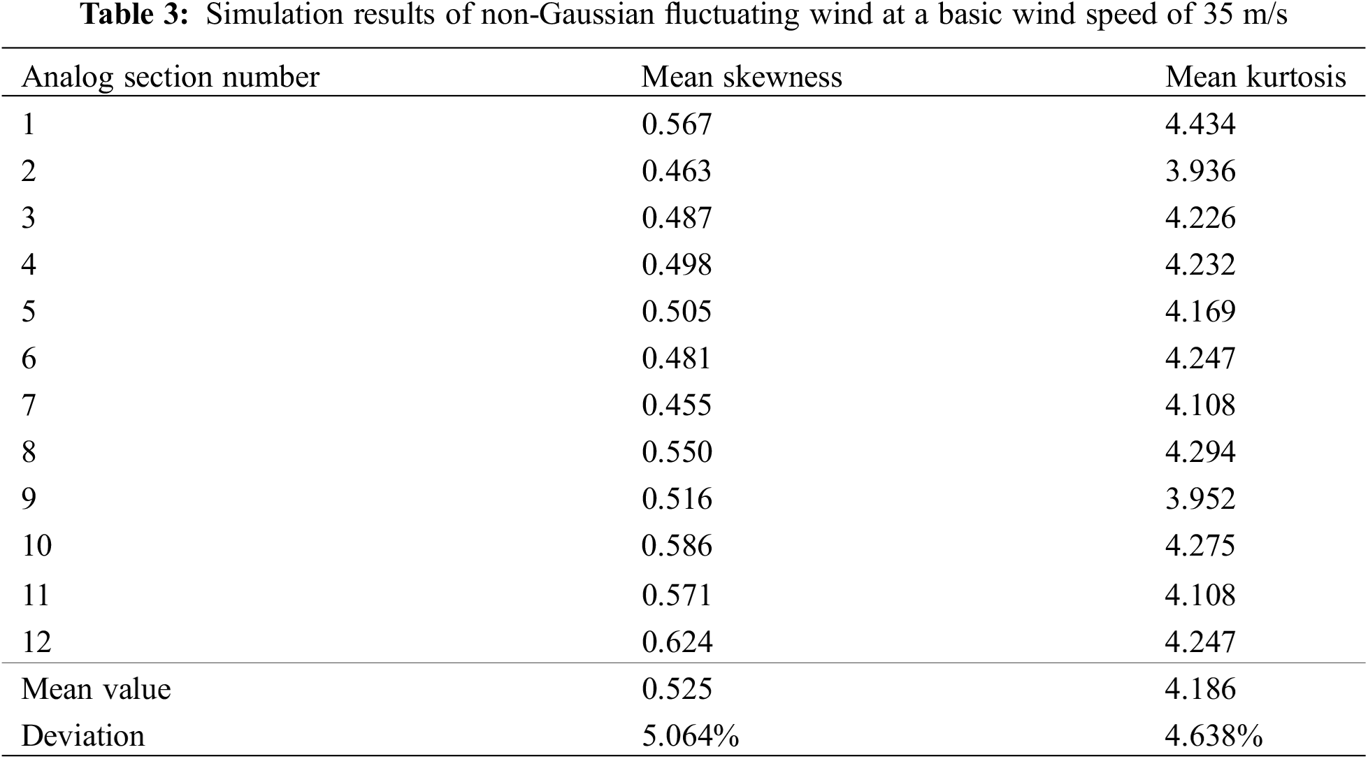
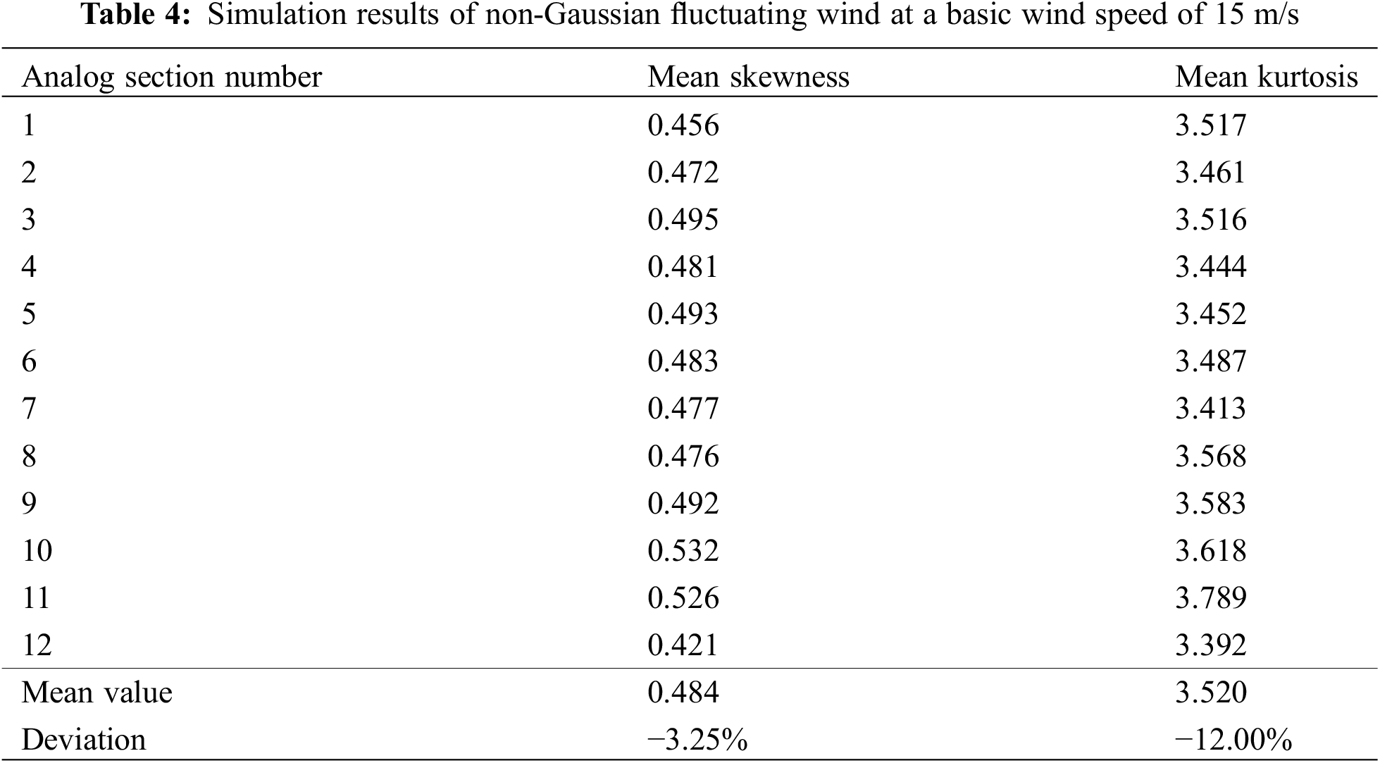
It can be seen that the skewness and kurtosis of wind speed data generated by numerical simulation of non-Gaussian wind are close to the target value, and the error is small, which proves that the generation method of non-Gaussian wind is reliable.

The wind speed results of specific sections can be analyzed by further testing the non-Gaussian fluctuating wind generation results. Extract the wind speed at the 10th section with a height of 21.0 m in a simulation, and the time series of its fluctuating wind speed is shown in Fig. 4. The skewness and kurtosis of the simulated wind speed are 0.4592 and 4.1214.

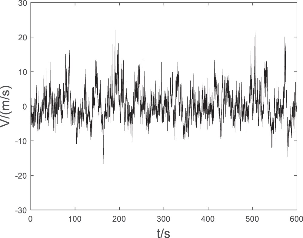
Figure 4: Fluctuating wind speed time series of simulation section 10

As can be seen, the fluctuating wind speed fluctuates around 0.

The Gaussian fluctuating wind speed series before the non-Gaussian conversion is compared with the non-Gaussian fluctuating wind speed series after the conversion, which is shown in Fig. 5. The red line represents the Gaussian wind speed series, and the black line represents the non-Gaussian wind speed series. It can be seen that the fluctuation range of the Gaussian wind speed series around 0 is small, while the fluctuation of the non-Gaussian wind speed series is wilder, and the change is more irregular.

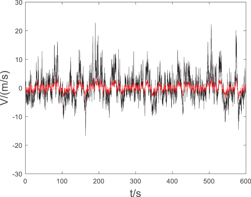
Figure 5: Gaussian and non-Gaussian fluctuating wind speed series

The simulation result of non-Gaussian fluctuating wind speed is compared with the Davenport power spectrum, and the result is shown as follows. It can be seen from Fig. 6 that the power spectrum of non-Gaussian fluctuating wind simulation results is generally consistent with the specified power spectrum, meeting the requirements of wind field simulation.

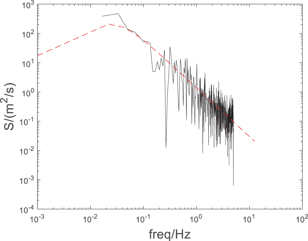
Figure 6: Comparison between computed power spectrum and Davenport power spectrum of simulation section 10

Due to the correlation of spatial wind field, it is also necessary to verify the spatial correlation of wind speed at different heights. The first section, with a height of 40.5 m, is selected as the benchmark. The spatial correlation between the wind speed of other sections and the simulation results of the first section is shown in Fig. 7.

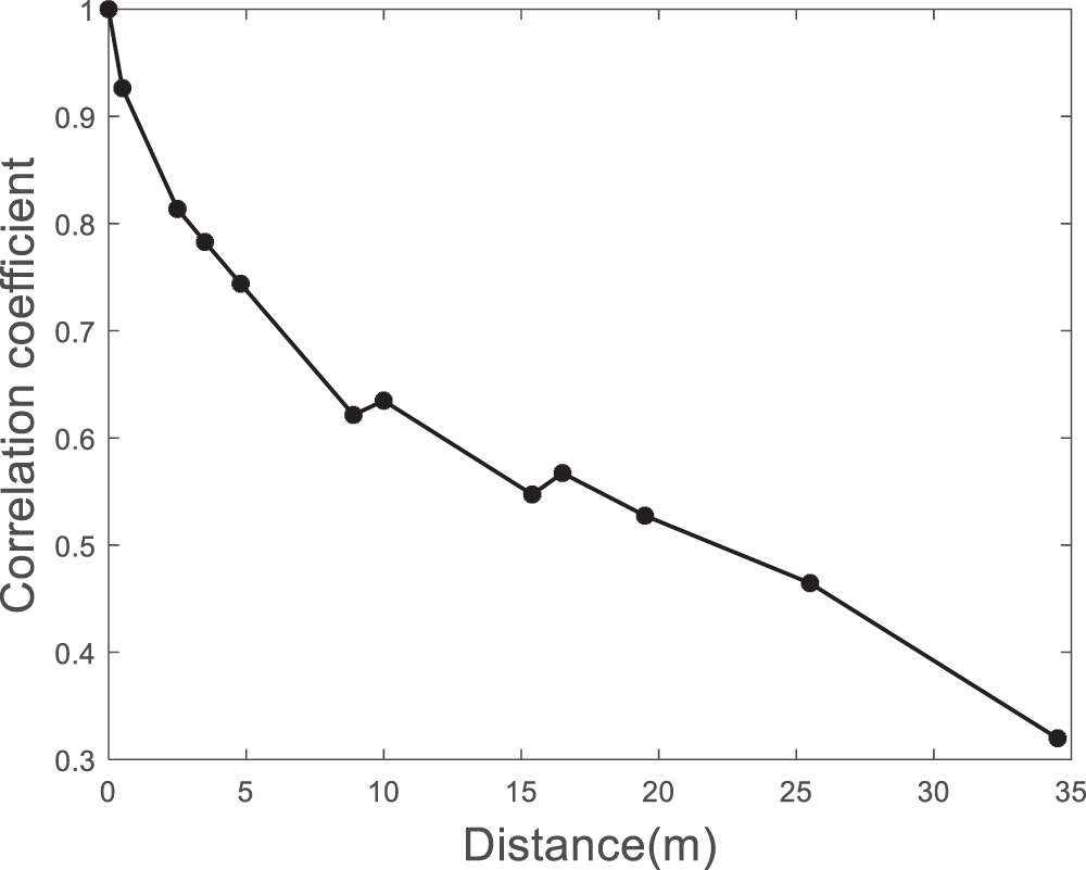
Figure 7: Figure of correlation coefficient of fluctuating wind speed between each section and section 1

Specific data of correlation coefficient are shown in Table 5.

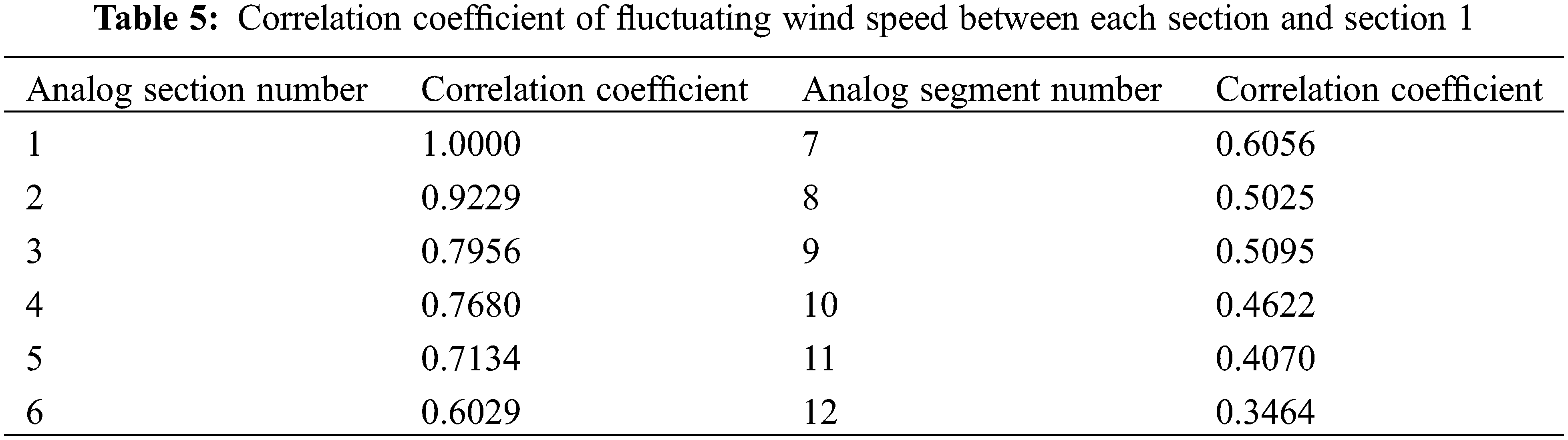
The spatial correlation of wind speed is related to the distance between two points. The farther the distance is, the weaker the spatial correlation is. The results of non-Gaussian wind simulation are consistent with this trend, and the simulation method is effective.

The kernel density estimation method is used to test the overall probability distribution of fluctuating wind speed, and the probability density distribution curve of simulated wind speed is obtained [31]. The histogram in Fig. 8a represents the generated fluctuating wind speed samples, the black line represents the fitting curve of the corresponding kernel density estimation method, and the red line represents the standard distribution curve.

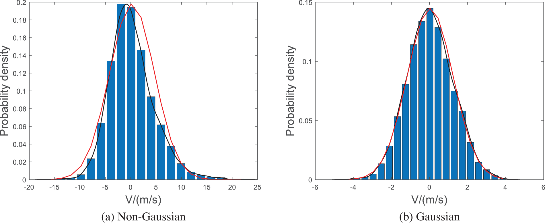
Figure 8: Verification of probability distribution form of simulation section 10

Compared with the normal curve of Gaussian distribution, the probability density distribution of non-Gaussian simulated wind speed is biased towards negative wind speed, which conforms to the wind speed distribution characteristics when the skewness is greater than 0, showing positive skewness characteristics. The probability density distribution curve of simulated wind speed is thinner than that of normal distribution, and its characteristics are consistent with the soft response process when the kurtosis is greater than 3.

Fig. 8b shows the probability distribution of Gaussian wind speed without non-Gaussian transformation. Compared with Fig. 8a, it can be seen that the Gaussian wind speed distribution conforms to the normal distribution. In contrast, the non-Gaussian wind speed distribution has a large deviation from the normal distribution, showing non-Gaussian characteristics.

To verify whether the coherence function of simulated non-Gaussian fluctuating wind speed at each point is consistent with the specified coherence function, the comparison between the coherence function of simulated fluctuating wind speed at 10 section and other sections and the specified coherence function is shown in Fig. 9. The specified coherence function specified is formula (6).

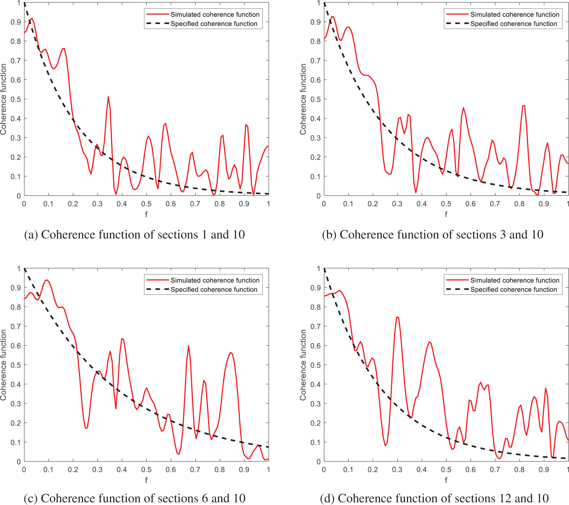
Figure 9: Coherence function between section 10 and certain remaining sections

As seen from Fig. 9, the coherence function of section 10 and each section generally shows a decreasing trend with the increase of frequency. The overall trend is in good agreement with the coherence function of the two sections in the specified space, indicating that the non-Gaussian fluctuating wind speed time series in each section meets the requirements of spatial correlation. It can be verified that the simulation accuracy meets the requirements.

The actual wind field consists of two parts: average wind and fluctuating wind. Therefore, to explore the wind-induced response of transmission tower lines in the actual environment, the average wind that varies with height should be added based on fluctuating wind. The time series of total wind speed in section 10 is shown in Fig. 10.

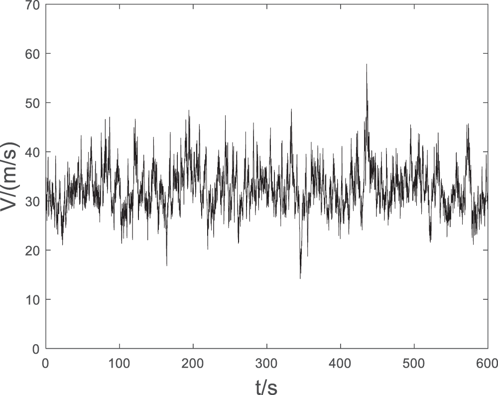
Figure 10: Result of spatial wind field generation in section 10

It shows that the overall spatial wind field fluctuates around the average wind speed, with non-Gaussian characteristics, which meets the target requirements. The simulation method of non-Gaussian wind is reliable and effective.

This paper improves and synthesizes the traditional numerical simulation method of fluctuating wind. Compared with the commonly used simulation method, the linear filter AR method is used to simulate multi-point Gaussian fluctuating wind speed, which clarifies the simulation process and reduces unnecessary steps, thus improving the calculation efficiency. In the process of non-Gaussian correlation transformation, the correlation between the calculation parameters h3 and h4 and the skewness and kurtosis is introduced to reduce the complexity of calculating the inverse function. The wind speed numerical simulation analysis is carried out on the transmission tower, and the reliability of the simulation results is verified. The final result can output the wind speed time series superimposed by average wind and fluctuating wind, which can be directly applied to the analysis of the wind vibration response of transmission towers and other structures.

5  Conclusion

Based on the characteristics of the actual spatial wind field, this paper summarizes the numerical simulation method of the spatial wind field and takes an actual transmission tower as an example to verify the simulation method. The conclusions are as follows:

1)   Considering the non-Gaussian characteristics of the spatial wind field, the appropriate power spectrum and calculation parameters are selected to improve the calculation method and improve the calculation efficiency. The wind speed numerical simulation method suitable for general spatial wind field is obtained;

2)   The mean wind is superimposed based on the fluctuating wind, which makes the results more consistent with the characteristics of the actual wind field environment, and provides the basic simulation conditions for the wind-induced response research of the transmission tower line system and power equipment;

3)   The characteristics of the probability distribution of wind speed simulation results are discussed, which provides ideas for the follow-up research on the actual wind field probability analysis.

Acknowledgement: The authors would like to thank the editor and reviewers for their valuable comments and suggestions.

Funding Statement: This work was supported by the Science and Technology Project of the State Grid Shanxi Electric Power Company (520530220005).

Author Contributions: The authors confirm contribution to the paper as follows: study conception and design: Yongxin Liu, Bo He; data collection: Jianxin Xu, Xiaokai Meng, Puyu Zhao; analysis and interpretation of results: Puyu Zhao, Yongxin Liu, Jianxin Xu; draft manuscript preparation: Puyu Zhao, Yongxin Liu, Hong Yang. All authors reviewed the results and approved the final version of the manuscript.

Availability of Data and Materials: The authors declared no potential conflicts of interest with respect to the research, authorship, and/or publication of this article.

Conflicts of Interest: The authors declare that they have no conflicts of interest to report regarding the present study.

References

1. Gao, Y. K. (2021). Numerical simulation research on typhoon wind field acting on transmission line site in eastern coastal mountainous area (Ph.D. Thesis). Shantou University, Shantou, China. [Google Scholar]

2. Xie, Q., Zhang, Y., Li, J. (2006). Investigation on tower collapses of 500 kV 5237 transmission line caused by downburst. Power System Technology, 2006(10), 59–63+89 (In Chinese). https://doi.org/10.13335/j.1000-3673.pst.2006.10.012 [Google Scholar] [CrossRef]

3. Luo, K. W., Zhang, H. J., Li, Y. S., Weng, L. X. (2021). Collapse analysis on 500 kV transmission tower under combined action of typhoon and microtopography. Journal of Physics: Conference Series, 2033, 012197. [Google Scholar]

4. Tao, T. Y., Wang, H., Wu, T. (2017). Comparative study of the wind characteristics of a strong wind event based on stationary and nonstationary models. Journal of Structural Engineering, 143(5), 40162305 (In Chinese). https://doi.org/10.1061/(ASCE)ST.1943-541X.0001725 [Google Scholar] [CrossRef]

5. Hao, J. M., Feng, Y., Su, Q. K., Han, W. S. (2022). Analysis and simulation of non-stationary typhoon field on long span bridge. Journal of Chang’an University (Natural Science Edition), 42(6), 66–76. https://doi.org/10.19721/j.cnki.1671-8879.2022.06.007 [Google Scholar] [CrossRef]

6. Duan, Z. Y. (2017). Wind characteristics with various topographies and wind effects of transmission lines systems (Ph.D. Thesis). Zhejiang University, Hangzhou, China. [Google Scholar]

7. Yan, Q., Li, J. (2011). Research on spatial coherence of stochastic wind field. Journal of Tongji University (Natural Science), 39(3), 333–339 (In Chinese). [Google Scholar]

8. Lorenzo, I. F., Elena, B. C., Rodríguez, P. M., Parnás, V. B. E. (2020). Dynamic analysis of self-supported tower under hurricane wind conditions. Journal of Wind Engineering & Industrial Aerodynamics, 197, 104078. [Google Scholar]

9. Zhang, X. M. (2011). Analysis and modeling of non-Gaussian fluctuating wind speed of typhoon based on field measurements (Ph.D. Thesis). Harbin Institute of Technology, Harbin, China. [Google Scholar]

10. Zhang, J. Q., Li, N., Gao, Y. L., Feng, W. T., Zhao, M. X. (2021). Study on numerical simulation of strong wind field in large field and inflow space. High Voltage Apparatus, 57(7), 98–104. https://doi.org/10.13296/j.1001-1609.hva.2021.07.014 [Google Scholar] [CrossRef]

11. Shen, G. H., Huang, Q. Q., Guo, Y., Xing, Y. L., Lou, W. J. (2013). Simulation methods of fluctuating wind field and its application in wind-induced response of transmission lines. Acta Aerodynamica Sinica, 31(1), 69–74. [Google Scholar]

12. Chang, G. C. (2015). Extreme response analysis of transmission tower under non-Gaussian wind (Ph.D. Thesis). Southwest Jiaotong University, Chengdu, China. [Google Scholar]

13. Kim, H., Shields, M. D. (2015). Modeling strongly non-Gaussian non-stationary stochastic processes using the iterative translation approximation method and Karhunen–Loève expansion. Computers and Structures, 161, 31–42. https://doi.org/10.1016/j.compstruc.2015.08.010 [Google Scholar] [CrossRef]

14. Wen, Q. (2020). Non-Gaussian stochastic process simulation based on spectral representation (Ph.D. Thesis). Shenzhen University, Shenzhen, China. [Google Scholar]

15. Jiang, L. (2019). Research on simulation algorithm of non-Gaussian stochastic process based on measured data (Ph.D. Thesis). Shanghai University, Shanghai, China. [Google Scholar]

16. Iannuzzi, A., Spinelli, P. (1987). Artificial wind generation and structural response. Journal of Structural Engineering, 113(12), 2382–2398. [Google Scholar]

17. Owen, J. S., Eccles, B. J., Choo, B. S., Woodings, M. A. (2001). The application of auto-regressive time series modelling for the time-frequency analysis of civil analysis structures. Engineering Structures, 23(5), 521–536. [Google Scholar]

18. Peng, G., Wang, X. (2010). Simulation of wind speed time-series using linear filter method and model order identification. Journal of Guangdong University of Technology, 27(2), 32–35 (In Chinese). [Google Scholar]

19. Li, Y. S., Kareem, A. (1993). Simulation of multivariate random processes: Hybrid DFT and digital filtering approach. Journal of Engineering Mechanics, 119(5), 1078–1098. [Google Scholar]

20. Grigoriu, M. (1998). Simulation of stationary non-Gaussian translation processes. Journal of Engineering Mechanics, 124(2), 121–126. [Google Scholar]

21. Gioffre, M., Gusella, V., Grigoriu, M. (2000). Simulation of non-Gaussian field applied to wind pressure fluctuations. Probabilistic Engineering Mechanics, 15(4), 339–345. [Google Scholar]

22. Wu, H. H., Mi, H. M. (2017). Research on fractal simulation of non-Gaussian fluctuating wind pressure. Journal of Hunan University (Natural Sciences2017, 44(7), 59–68. https://doi.org/10.16339/j.cnki.hdxbzkb.2017.07.008 [Google Scholar] [CrossRef]

23. Zhang, Y. J. (2021). Non-Gaussian stochastic process simulation and its application in wind disaster vulnerability analysis of transmission tower structure (Ph.D. Thesis). Chongqing University, Chongqing, China. [Google Scholar]

24. Luo, Y., Ren, D. C., Han, Y., Dong, G. C. (2022). Study on buffeting response of bridge under non-Gaussian wind field. Acta Aerodynamica Sinica, 41(8), 107–116. [Google Scholar]

25. Cai, W. S. (2021). Study on dynamic response of wind turbine with pile foundation considering non-Gaussian characteristics of wind load (Ph.D. Thesis). Southeast University, Nanjing, China. [Google Scholar]

26. Chen, B. (2021). Vulnerability analysis of transmission tower structure based on kriging surrogate model (Ph.D. Thesis). Huazhong University of Science and Technology, Wuhan, China. [Google Scholar]

27. Zhang, H. X., Ye, F., Gu, M. (2003). Experimental investigation on coherence characteristics of along-wind fluctuating wind velocity and wind pressure. The Eighth National Conference on Vibration Theory and Application, vol. 1. China. [Google Scholar]

28. Yuan, B., Ying, H. Q., Xu, J. W. (2007). Simulation of turbulent wind velocity based on linear filter method and matlab program realization. Structural Engineers, 23(4), 55–61. https://doi.org/10.15935/j.cnki.jggcs.2007.04.004 [Google Scholar] [CrossRef]

29. Ma, X. L. (2015). Research of non-Gaussian characteristics of bridge wind loads (Ph.D. Thesis). Dalian University of Technology, Dalian, China. [Google Scholar]

30. Grigoriu, M. (2008). A class of weakly stationary non-Gaussian models. Probabilistic Engineering Mechanics, 23(4), 378–384. [Google Scholar]

31. Fu, Q., Kuang, W. K., Xue, Y., Yang, Y. N., Su, S. (2021). Detection method for street lamp electricity theft based on Gaussian kernel density estimation. Proceedings of the CSU-EPSA, 33(10), 18–23. https://doi.org/10.19635/j.cnki.csu-epsa.000609 [Google Scholar] [CrossRef]