Prediction and Analysis of Vehicle Interior Road Noise Based on Mechanism and Data Series Modeling

1  Introduction

Amidst the escalating challenges of global environmental pollution and the concurrent energy crisis, the incorporation of energy-efficient and environmentally sustainable pure electric vehicles has emerged as a pivotal consideration in the eco-friendly evolution of the automotive industry. Specifically, pure electric vehicles, devoid of engine-generated excitation noise, exhibit heightened sensitivity to road noise, particularly within low and medium frequency ranges [1]. The prolonged exposure to road noise generated during vehicular operation not only compromises ride comfort but also poses potential risks to human well-being [2]. Consequently, road noise has become a paramount concern within the realm of noise, vibration, and harshness considerations (NVH), garnering substantial attention from leading manufacturers of pure electric vehicles [3]. The suspension system, as a critical component in vehicular vibration and noise mitigation, plays a pivotal role in dampening the impact vibrations induced by uneven road surfaces. A well-designed suspension not only ensures efficient force transmission between the wheel and chassis but also enhances overall ride comfort and handling stability. Its performance directly influences the driving experience of vehicle users, underscoring the importance of a comprehensive investigation into suspension systems with both practical and engineering relevance.

Historically, due to technological constraints, scholars often elucidated the correlation between suspension systems and vehicular vibration performance through the establishment of mathematical models. In the mid-20th century, notable figures, such as Olley [4], Segel [5] in the United States, and Matschinsky [6] in Germany made seminal contributions to the field of suspension. As scientific and technological progress advanced, Wang [7] established an eight-degree-of-freedom vehicle vibration mathematical model by simplifying the complex vehicle system. Li et al. [8] proposed a hybrid vehicle suspension structure with springs, dampers, and inverters. Simultaneously, Hurel et al. [9] put forward a planar quarter-car analytical model considering geometry and tire modeling. While such mechanical analysis models simplify and clarify certain scenarios, subsequently reducing computational overhead, significant discrepancies may arise in analytical outcomes in numerous cases. With the increasing complexity of vehicle dynamics models and the proliferation of differential equations, this is particularly evident. In this case, the modeling, analysis and analysis of mathematical models have become a key issue.

With the continual evolution of computer technology, Computer-Aided Engineering (CAE) technology is now extensively employed in the automotive sector through computer programs. In comparison to traditional mathematical models, the widespread use of CAE not only facilitates the construction and analysis of multi-degree-of-freedom models of automobiles but also expands the scope of simulation analysis applications. Conventional vehicle modeling approaches often involve reducing individual vehicle components to rigid bodies [10], resulting in low modeling accuracy. The introduction of finite element technology, however, ushered in the era of rigid-flexible coupling analyses for dynamic vehicle models. Scholars, such as Chen et al. [11,12], Chang et al. [13], and Wang et al. [14] utilized mechanical system dynamics simulation software ADAMS in conjunction with finite element analysis software to model, simulate, and optimize the dynamic behavior of entire vehicles. While the multi-body dynamic model of the entire vehicle demonstrates commendable modeling efficiency, it lacks direct capability in ascertaining the vehicle’s interior noise. Furthermore, finite element technology has been directly applied to prognosticate the road noise performance of vehicles. For example, Zeng et al. [15] and Yang et al. [16] constructed a finite element model of the whole vehicle to analyze road noise and optimize the suspension structure. Despite the commendable fidelity and precision of the finite element model of the entire vehicle, it is marked by comparatively diminished modeling efficiency. The research is based on a mechanistic model for computation, but relying purely on the mechanism model has considerable limitations due to the fact that the abstraction and idealization of the model make the modeling inadequate, and it requires a lot of manpower and material inputs if it is to be done accurately. Therefore, the hope of purely mechanism modeling for endpoint prediction is susceptible to more interference, which leads to a more difficult trade-off between accuracy and efficiency.

In contemporary times, machine learning has emerged as a pivotal technical underpinning across diverse domains, finding extensive applications in both scientific research and engineering disciplines [17–20]. Notably, within the realm of automotive NVH, machine learning has demonstrated noteworthy efficacy. Huang et al. [21] and Liu et al. [22] employed the improved residual network and Long Short-Term Memory (LSTM), respectively, to predict road noise problems. Lin et al. [23] demonstrated that the combination of multifractal detrended fluctuation analysis and support vector machine has great potential for fault diagnosis of gearboxes. Data-driven machine learning methods have introduced a transformative solution to the modeling of nonlinear dynamical systems in the automotive domain. While mechanism modeling approaches rely on explicit knowledge of system dynamics, data-driven methods construct equivalence laws between state variables based on historical operational data. This approach, while versatile and adept at uncovering latent features, exhibits a reliance on data scale and may exhibit limited generalization performance [24].

First, for a better trade-off between accuracy and efficiency, this paper will build an efficient rigid-flexible coupled vehicle dynamics model and connect it in series with the data-driven model. This is done by adding the data generated from the dynamic model to the data-driven dataset. This approach not only avoids highly complex structure–acoustic coupling analysis, but also solves the problem that multi-body dynamics models need to obtain in-vehicle noise through complex modeling. Meanwhile, the accuracy and convergence of the data-driven model are improved by increasing the effective sample size. Second, considering that road noise involves multiple features, an algorithmic framework combining autoencoder (AE) and LSTM is explored, which can extract robust features from the dataset. It is shown that the LSTM unit can capture the dependencies in the data, and the AE module can reduce the noise interference in the data, thus realizing more accurate and efficient in-vehicle noise prediction.

The contributions of this study are delineated as follows: (1) Facing the problem of coordinating the accuracy and efficiency of testing and simulation analysis in engineering, based on the serial modeling of mechanistic model and data-driven model, combining the advantages of high efficiency of dynamics in solving vibration as well as the ability of the data-driven model to fit the complex nonlinear problems, the method of automobile road noise prediction combining the knowledge and the data is proposed. (2) Considering that road noise involves more features, the prediction using the LSTM model will be affected by some redundant features, which pulls down the computational efficiency, therefore, this paper introduces an autoencoder (AE) on the basis of the LSTM model, and establishes an AE-LSTM model oriented to the analysis of road noise, which is used for the prediction of driver’s right ear noise.

The paper is organized as follows: Section 2 elucidates the modeling process of the multi-body dynamic model, explicating the establishment of the AE-LSTM prediction model, and providing an in-depth exposition of the research methodology, delineating the framework of the series model. Section 3 outlines the specific procedures employed for the acquisition of body side vibration acceleration data and interior noise data from an automotive source, employing experimental techniques, and presents the ensuing data outcomes. Section 4 is dedicated to the discussion and analysis of the results, encompassing the validation of the accuracy of the multi-body dynamic model, the demonstration of the AE-LSTM prediction outcomes, and the substantiation of the efficiency and precision of the series modeling approach. Finally, Section 5 furnishes a comprehensive summary of the research content encapsulated within this article.

2  Research method

2.1 Establishment of Dynamic Model for Vehicle Interior Noise

The vehicle assembly model encompasses the front MacPherson suspension system, the rear three-link suspension system, the body system, the steering system, the powertrain system, and the tire system. To faithfully replicate the operational conditions of the components and construct a precise multi-body dynamics model, this paper will combine the road noise analysis frequency band requirements (25–250 Hz), in the cut-off frequency band (generally the upper limit of the cut-off frequency is 2 times of the upper limit of the analysis frequency [25], this paper selects 350 Hz as the upper limit of the cut-off frequency) to screen the free modes of the front and rear suspension components and the body, and then according to the screening results, the corresponding components are flexible. The free modes of the body and suspension structures are summarized in Table 1, and since the first 6 orders are rigid body modes, we start the analysis from the 7th order structural modes. The body, subframe, and anti-roll bar have more modal frequencies within the cut-off frequency (350 Hz), and only some of their modal orders and modal frequencies within the cut-off frequency are listed in the table, and the parts exceeding the cut-off frequency are indicated by “>350 Hz”. Meanwhile, since the seventh-order natural frequencies of the front control arm, rear upper control arm, rear lower control arm, and rear trailing arm are larger than the cut-off frequency, the interior noise within the analyzed frequency band will not be caused by the modes of these four parts, so the table does not show the modal information in detail, and it is only indicated by “>350 Hz”. According to the principle that the non-rigid free mode of the internal parts in the cut-off frequency range needs to be flexible, the following components that need to be flexible are: front subframe, rear subframe, front anti-roll bar, rear anti-roll bar and body.

Based on the above analysis results, the vehicle rigid-flexible coupling model can be established, in which the rigid-flexible coupling model of front MacPherson suspension, rigid-flexible coupling model of rear three-link suspension, the body finite element model and the anti-roll bar finite element model are shown in Fig. 1 Each subsystem can be assembled to form a complete vehicle rigid-flexible coupling model, as shown in Fig. 2. It should be noted that the bushings used in the suspension and subframe models are rubber bushing elements containing dynamic stiffness characteristics, which can be modeled by the ADAMS/Ride module [26]. The constructed bushing model consists of the following three parts: the non-linear spring model: to provide the static stiffness characteristics and the nonlinear characteristics under the large deformation of the bushing, the Bouc-Wen model: to simulate the hysteresis effect of the bushing, and the Transfer function model: to simulate the frequency dependence of the bushing. Based on this, the identified bushing stiffness curve and loss angle curve are shown in Fig. 3.

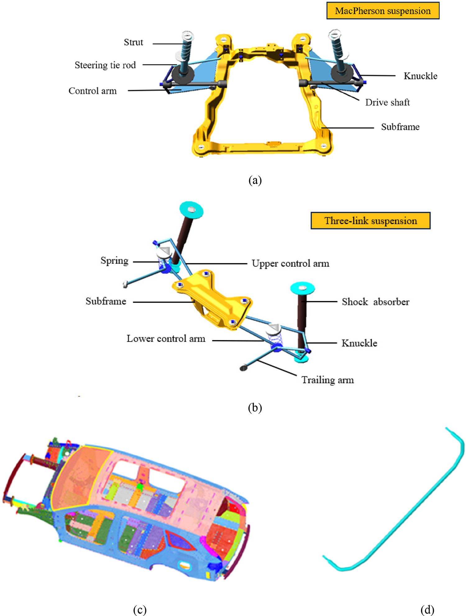
Figure 1: Component structure. (a) MacPherson suspension. (b) Three-link suspension. (c) Body finite element model. (d) Anti-roll bar finite element model

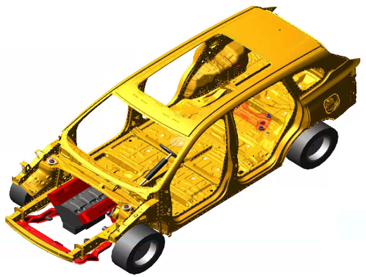
Figure 2: Rigid-flexible coupling model of the whole vehicle

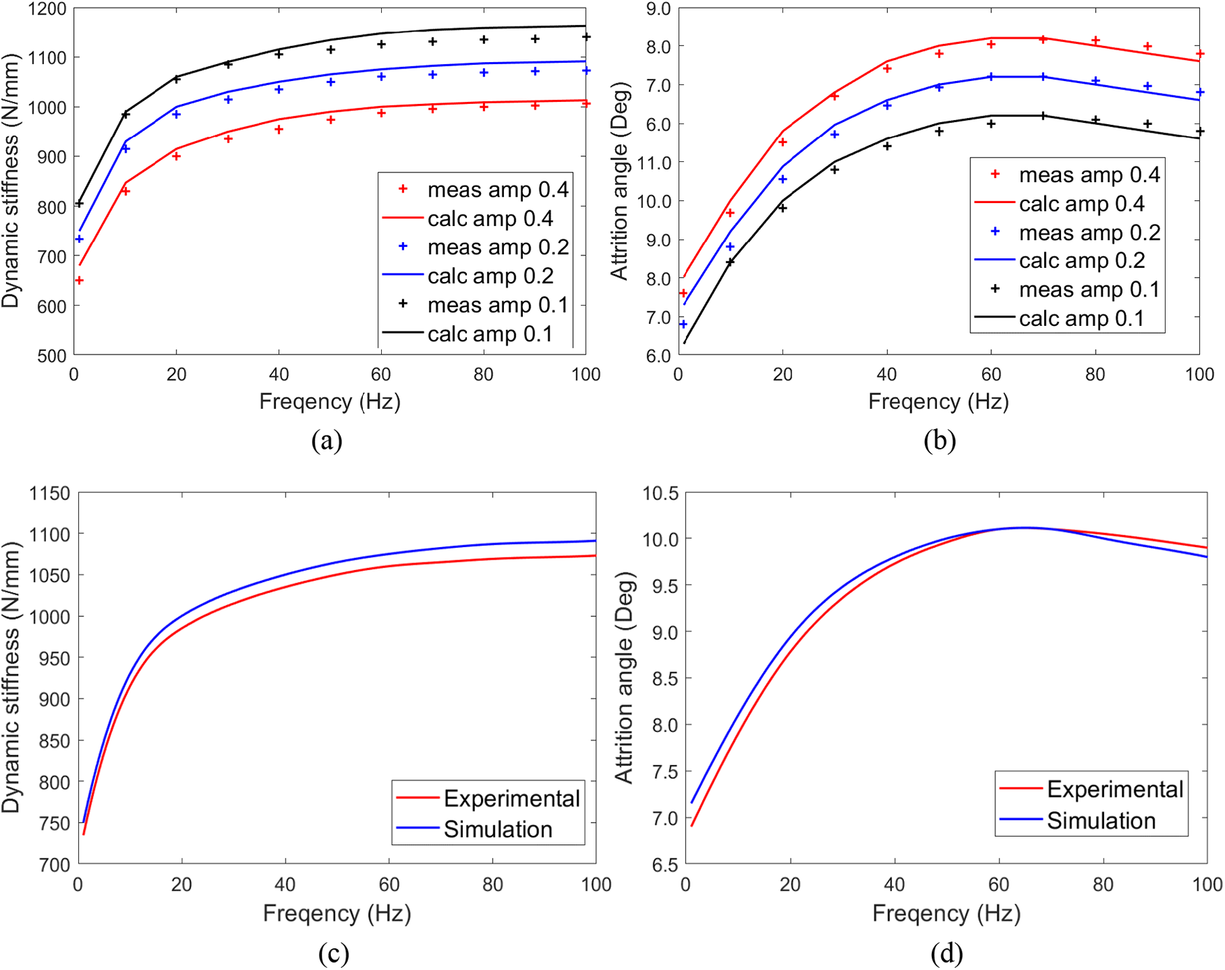
Figure 3: Identification results of x-direction parameters of the rear bushing of the control arm. (a) The x-direction dynamic stiffness curve of the rear bushing of the control arm. (b) The x-direction loss angle curve of the rear bushing of the control arm. (c) Comparison of simulated and experimental dynamic stiffness for an amplitude of 0.2 mm. (d) Comparison of simulated and experimental loss angles for an amplitude of 0.2 mm
Note: meas amp 0.1 is the dynamic stiffness at an amplitude of 0.1 mm for the test, calc amp 0.1 is the dynamic stiffness at an amplitude of 0.1 for the identification calculation. Similarly, meas amp 0.2, calc amp 0.2, meas amp 0.4, and calc amp 0.4.

In addition, for subsequent data-driven modeling analysis, it is imperative to acquire vibration acceleration data from specific points, including the front strut to body connection point body side, front subframe to body front connection point body side, front subframe to body rear connection point body side, rear subframe to body front connection point body side, rear subframe to body rear connection point body side, rear shock absorber to body connection point body side, rear spring to body connection point body side, and rear trailing arm to body connection point body side acceleration. Therefore, when creating suspension and subframe models, it is necessary to establish marker points and sensors at the corresponding position on the body side. In the simulation, the ADMAS/Ride module is used to establish a B-level random road surface based on the Sayers empirical digital formula [27]. The road profile parameters Ge = 0, Gs = 12, and Ga = 0.17 are set. The simulation speed is 60 km/h, the time is 10 s, and the sampling frequency is 1000 Hz. The parameters required for the above modeling process are provided by the Changan Automotive Global R&D Center.

2.2 Establishment of Interior Road Noise Prediction Model Based on AE-LSTM

The body-side vibration acceleration and the driver’s right ear noise were used as inputs and outputs of the prediction model, respectively, and the frequency range was set to 20–250 Hz. Given the extended nature of the road noise sequence spanning this frequency spectrum, conventional neural networks yield suboptimal results in predicting such prolonged sequences [28]. Consequently, the vehicle interior road noise prediction model leverages LSTM networks [29] to attain precise prognostication of the road noise sequence data.

As an advanced iteration of Recurrent Neural Networks (RNNs), LSTM has garnered widespread application across diverse domains, owing to its remarkable proficiency in handling sequential data [30–32]. It effectively mitigates the challenges of gradient vanishing and explosion encountered by RNNs when addressing long-term dependencies, achieved through the incorporation of specialized memory cells within the hidden layer unit. These memory cells feature self-connections for retaining temporal network states and are regulated by three gate mechanisms: the input gate, the output gate, and the forget gate. The architectural configuration of an LSTM block at a discrete time step is presented in Fig. 4, while the corresponding mathematical expressions are detailed in Eqs. (1) to (6).

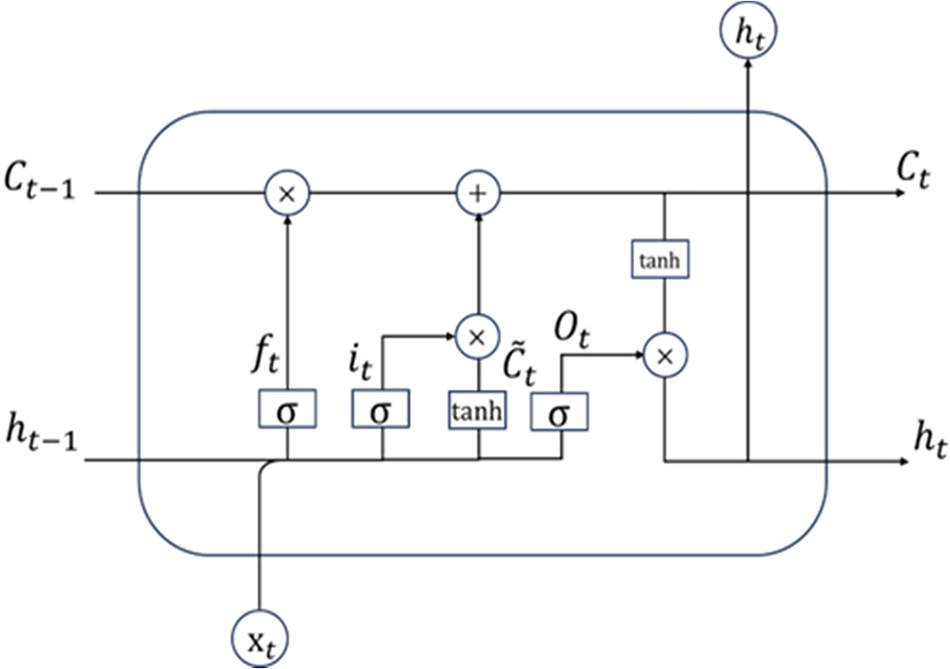
Figure 4: The structure of an LSTM block

The forget gate makes the decision of preserving/removing the existing information, defined as follows:

ft=σ(Wf[ht−1,xt]+bf)  (1)

where, ft is the output of the forget gate, σ represents the sigmoid activation function, Wf is weight matrices, ht−1 is the output value of the LSTM unit at the previous time, xt represents the input, bf is the bias value.

The input gate makes the decision of whether to add new information to the LSTM memory, defined as follows:

it=σ(Wi[ht−1,xt]+bc) (2)

Ct~=tanh(Wc[ht−1,xt]+bt)   (3)

where, itis the output of the input gate, σrepresents the sigmoid activation function,Wiis weight matrices, ht−1 is the output value of the LSTM unit at the previous time, xt represents the input, bc is the bias value, Ct~ is the new state of memory cell, tanh represents the tanh activation function, Wc is weight matrices, bt is the bias value.

Among them, Ct is selectively updated by the calculation results of the forget gate and the input gate, defined as follows:

Ct=ft⊗Ct−1+it⊗Ct~  (4)

where, Ct is the final state of memory cell, ft is the output of the forget gate, Ct−1 is the old state of memory cell, it is the output of the input gate, Ct~ is the new state of memory cell, ⊗ represents the point-wise multiplication.

The output gate can output information selectively as needed, defined as follows:

Ot=σ(Wo[ht−1,xt]+bo) (5)

ht=Ot⊗tanh⁡(Ct) (6)

where, Ot is the output of the output gate, σ represents the sigmoid activation function, Wo is weight matrices, ht−1 is the output value of the LSTM unit at the previous time, xt represents the input, bo is the bias value, ht is the new output value of the LSTM unit, Ct is the final state of memory cell, ⊗ represents the point-wise multiplication.

AE is an algorithm in unsupervised learning, which can automatically learn features from unlabeled data, it is a kind of neural network with the goal of reconstructing the input information, which can give better feature descriptions than the original data, and has a strong feature learning ability. In deep learning, good results have been achieved by using features generated by AE instead of original data [33–35]. In this paper, we introduce that AE processing the data before inputting it into the LSTM model can provide a variety of benefits, which including but are not limited to, improving data representation, reducing the impact of redundant features, and reducing the risk of model overfitting. These benefits enable LSTM model to better fit the data when applied to data processing tasks and improve model performance and prediction accuracy.

The AE-LSTM model consists of two parts, the first part is the encoding part of the AE model, whose main role is to generate the sequence data that can be input into the LSTM prediction model, and the second part is the LSTM model, whose main role is to predict the feature data extracted from the AE model. The AE-LSTM model can be realized by the following steps, where Fig. 5 is a schematic diagram of the structure of the AE-LSTM model and Eqs. (7) to (9) are the used equations.

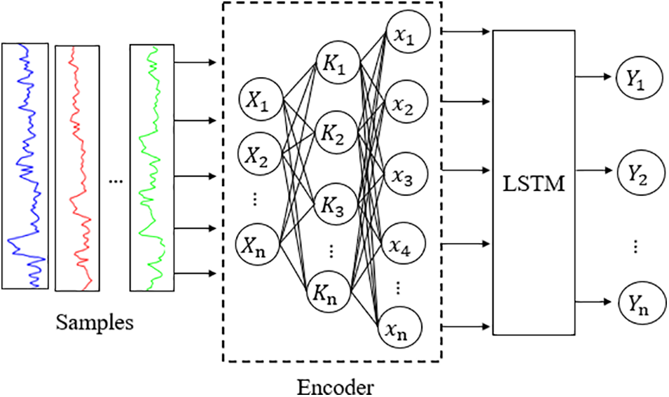
Figure 5: Structure diagram of the AE-LSTM model

The first step is to input the original data X(t) into the AE model for training, and use the encoding process to calculate the encoding data.

X^(t)=fdec(fenc(X(t)))  (7)

x(t)=fenc(X(t)) (8)

where, X(t) is the original input sequence data, X^(t) is the output of the decoder, x(t) is the output of the encoder, the superscript dec represents decoding, fdec(⋅) is the decoding function, the superscript enc represents encoding, and fenc(⋅) is the encoding function.

The second step: input x(t) into the LSTM model to obtain the output value Y(t).

Y(t)=fLSTM(x(t)) (9)

where, x(t) is the output of the encoder, Y(t) is the LSTM prediction output, the superscript LSTM represents the LSTM model, and fLSTM(⋅) is the LSTM function.

2.3 A Series Model Framework for Vehicle Interior Noise Prediction

Mechanism and data series modeling is to connect the mechanism model with the data-driven model in series to realize the analysis and prediction of vehicle vibration and noise. In this paper, a vehicle road noise prediction series architecture is proposed. As shown in Fig. 6, the mechanism model in the figure is the lower layer of the series model, whose modeling parameters include Geometric parameter (dimensional parameters and hard point coordinates of the control arm, steering tie rod and knuckle), Quality parameter (inertial moment, mass and center of mass of the control arm, steering tie rod and knuckle), External parameter (road parameter), and Mechanical parameter (damping characteristics of the damper, stiffness of springs, bushings and limit blocks), and the extracted parameters are the vibration acceleration at each measurement point of the body side (the front strut to body connection point body side, front subframe to body front connection point body side, front subframe to body rear connection point body side, rear subframe to body front connection point body side, rear subframe to body rear connection point body side, rear shock absorber to body connection point body side, rear spring to body connection point body side, and rear trailing arm to body connection point body side, and rear trailing arm to body connection point body side acceleration). For the data-driven model, the input is the vibration acceleration at each measurement point on the body side, and the output is the noise at the driver’s right ear. The vibration acceleration at each measurement point on the body side is used as both the output of the mechanism model and the input of the data-driven model, which serves as a bridge between the two models. Therefore, a series model with mechanism model modeling parameters as input and driver ‘s right ear noise as output is built. This method not only solves the limitations of the mechanism model in terms of accuracy and efficiency, but also solves the problem of lack of effective data for the data-driven model.

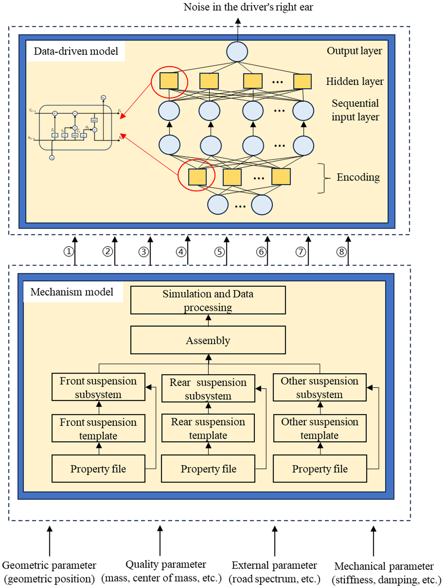
Figure 6: Series model architecture for vehicle interior noise prediction
Note: ① Front strut to body connection point body side acceleration. ② Front subframe to body front connection point body side acceleration. ③ Front subframe to body rear connection point body side acceleration. ④ Rear subframe to body front connection point body side acceleration. ⑤ Rear subframe to body rear connection point body side acceleration. ⑥ Rear shock absorber to body connection point body side acceleration. ⑦ Rear spring to body connection point body side acceleration. ⑧ Rear trailing arm to body connection point body side acceleration.

3  Experimental Tests

3.1 Test Scheme

In order to collect the road noise sample data and verify the accuracy of the vehicle dynamic model, a real vehicle road test is required. The experimental samples are constructed by Latin hypercube experimental design [36]. The design variables are the dynamic stiffness of the front suspension to body connection point bushings, dynamic stiffness of the rear suspension to body connection point bushings, dynamic stiffness of the front subframe to body connection point bushings, dynamic stiffness of the rear subframe to body connection point bushings, front shock absorber damping, and rear shock absorber damping. The test object is a class A vehicle and the vehicle meets the technical requirements of vehicle operation safety. The experimental equipment includes Leuven Measurement Systems (LMS) digital acquisition front-end, non-directional BSWA sound pressure microphone (model: MPA201-550507) and PCB three-way vibration sensor (model: BW13510-J0810/BW13510-J0812).

In order to collect the vibration data at the body structure and the noise data in car, the acceleration sensors are arranged on suspension to body connection point body side and subsystem to body connection point body side. All the sensors of the vehicle are arranged as shown in Fig. 7. The sound pressure microphone is arranged in the driver’s right ear, its vertical coordinates for the seat surface and the backrest surface of the intersection of the line directly above (0.7 ± 0.05) m, the horizontal coordinates in the center of the seat face to the right at a distance of (0.20 ± 0.02) m, as shown in Fig. 8. After all the test points are arranged, set the parameters of the data acquisition system, in order to accurately respond to the correspondence between the two signals and ensure that the data volume is not excessively redundant, the sampling time is set to 10 s, and the sampling frequency of noise and vibration signals is set to 1000 Hz, with a resolution of 1 Hz.

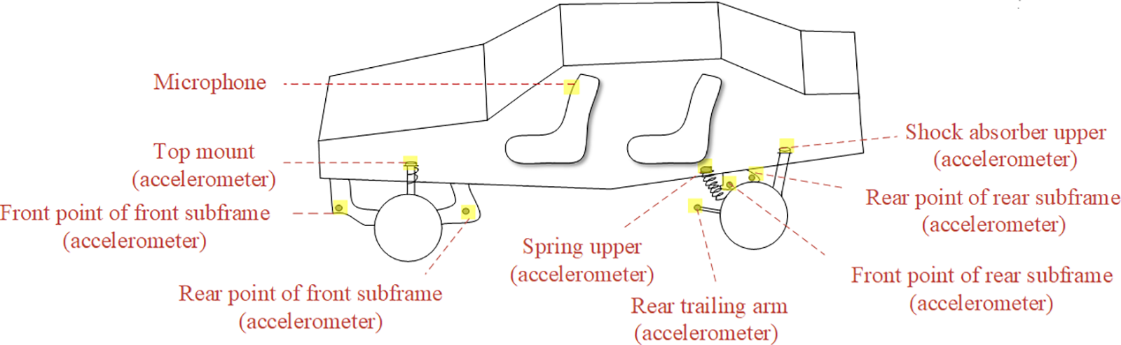
Figure 7: Sensors in the whole vehicle

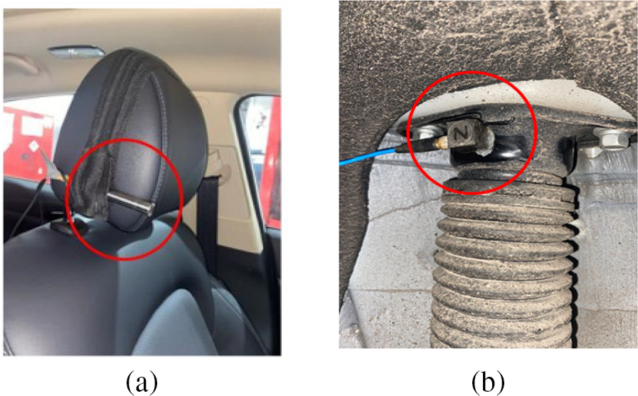
Figure 8: Sensor layout. (a) Layout of sound pressure microphone. (b) Layout of rear shock absorber to body connection point body side sensor

Synchronous acquisition of vehicle noise and vibration data through real vehicle road test. In order to make the vehicle response significantly during the test, the vehicle is selected to travel on the rough asphalt pavement at a uniform speed of 60 km/h. According to the test requirements, there are no three-dimensional buildings and other large objects that can reflect the noise within 20 m on both sides of the road, and the road condition is shown in Fig. 9. During the test, Belgium LMS software was used to collect data online and perform data analysis and processing. Through multiple tests, 40 sets of road noise and vibration data were collected, and the LMS software was used to convert the time-domain data of the interior road noise collected in the test into frequency-domain curves. The vibration acceleration curve with a resolution of 1 Hz and a frequency range of 0 to 250 Hz and the sound pressure curve of 20 to 250 Hz are derived.

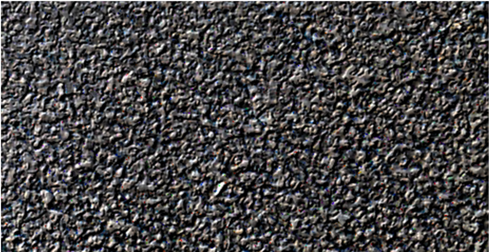
Figure 9: Rough asphalt pavement

3.2 Test Results

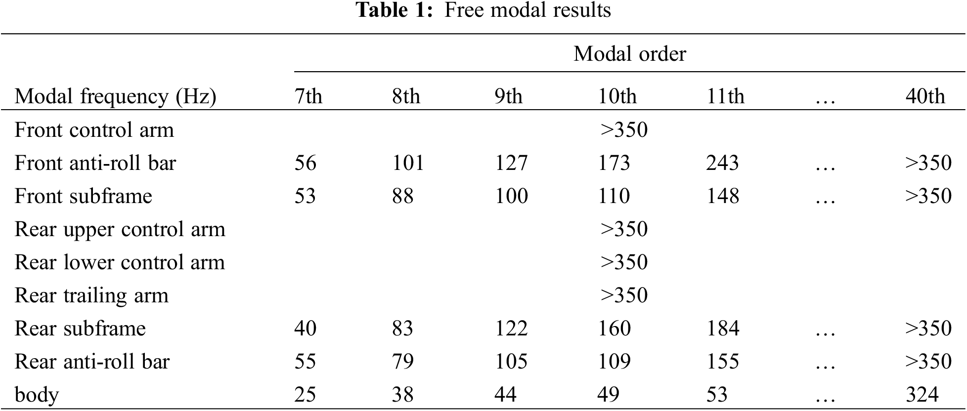
The interior noise of the vehicle and the vertical vibration of front subframe to body front connection point body side, rear subframe to body front connection point body side, front strut to body connection point body side and rear spring to body connection point body side are shown in Figs. 10 and 11, respectively. Due to the large number of test results, the text only lists some of them. As can be seen from Fig. 10, in the frequency range of 20–250 Hz, there are multiple resonance peaks in the sound pressure level curves of the right ear noise extraction points, with the peaks appearing at 25, 64, 111, 127, 211, and 226 Hz, respectively, of which the maximum sound pressure occurs at 25 Hz, with a value of 74.76 dB, and the peaks appear more densely in the frequency range of 50–150 Hz. The peaks in the frequency range of 50–150 Hz are more intensive. Combined with the results of modal analysis in Table 1, the peaks of interior noise at 25, 64, 111, 127 and 226 Hz are mainly caused by the body modes; and the peak at 211 Hz is mainly caused by the rear subframe modes. In addition, as shown in Fig. 11a, because the front subframe has a natural frequency at 166 Hz, the vibration response of the front subframe to body front connection point body side has a resonance peak at 166 Hz; as shown in Fig. 11b, the rear subframe has natural frequencies at 83 and 211 Hz, so the vibration response of the rear subframe to body front connection point body side has resonance peaks at 83 and 211 Hz. Similar characteristics are found for the front strut and the rear spring, as shown in Figs. 11c and 11d.

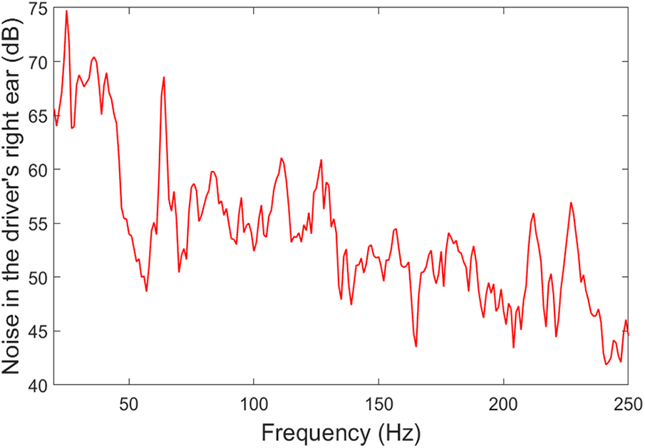
Figure 10: Noise in the driver’s right ear

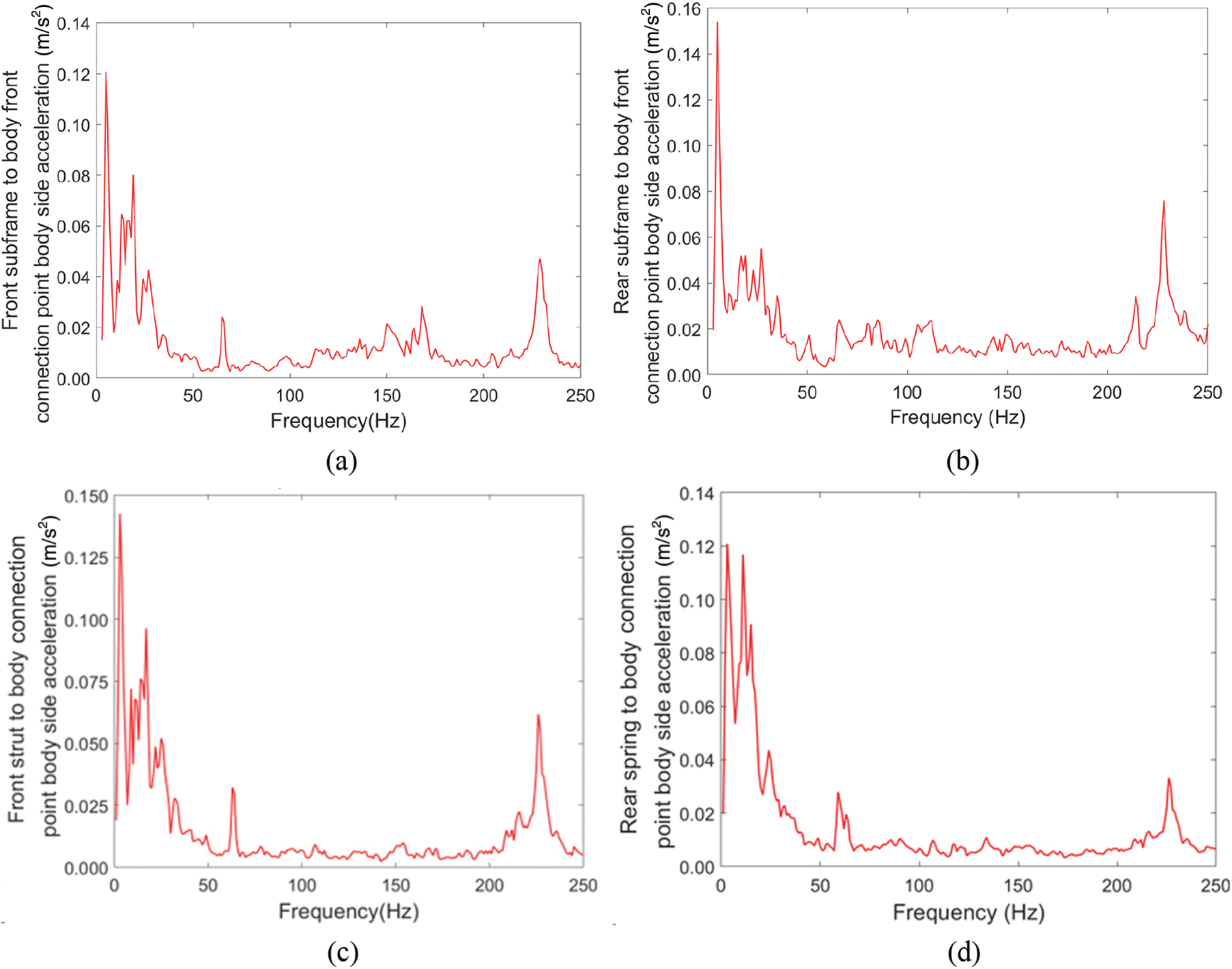
Figure 11: Vibration acceleration test results. (a) Front subframe to body front connection point body side acceleration. (b) Rear subframe to body front connection point body side acceleration. (c) Front strut to body connection point body side acceleration. (d) Rear spring to body connection point body side acceleration

4  Results Discussion and Analysis

4.1 Dynamic Model Verification for Vehicle Interior Road Noise

The initial step involves a rigorous validation of the dynamic model pertaining to interior road noise within the vehicle. The vehicle dynamics model is simulated under conditions as closely aligned as possible with the test conditions, yielding vibration acceleration data at each measuring point. A comparison between the simulated vibration acceleration results and those measured during the test is conducted to verify the reliability of the vehicle dynamics model. Fig. 12 illustrates a comparative analysis of vibration accelerations between the vehicle’s rigid-flexible coupling model and the actual test vehicle, both traveling at a consistent speed of 60 km/h. Focusing on key connection points, such as the front subframe to body front connection point, front strut to body connection point, rear subframe to body rear connection point, and rear shock absorber to body connection point, the comparison reveals a congruence in acceleration trends. Notably, the simulation curves adeptly capture peak effects at frequencies of 25, 64, and 226 Hz, with relative errors in peak amplitudes well within 10%. Furthermore, absolute errors in peak frequency points remain within a 2 Hz margin. Consequently, the simulation and test curves exhibit commendable alignment, affirming the capacity of the whole car’s rigid-flexible coupling model to accurately compute the vibrational characteristics of the vehicle under uniform linear motion conditions.

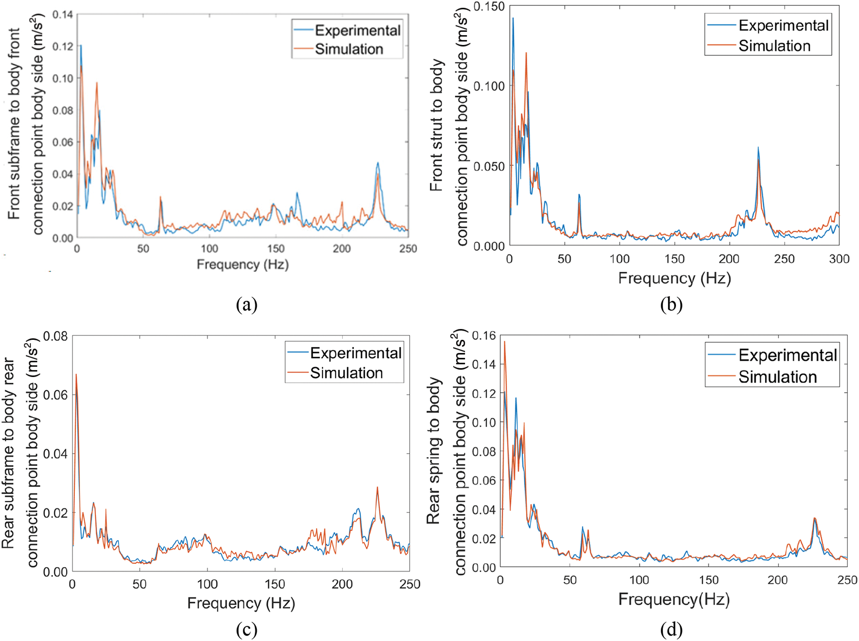
Figure 12: Comparison of simulation and experimental results. (a) Front subframe to body front connection point body side acceleration. (b) Front strut to body connection point body side acceleration. (c) Rear subframe to body rear connection point body side acceleration. (d) Rear spring to body connection point body side acceleration

4.2 Series Model Interior Noise Prediction Results

Moreover, this study conducts the prediction and validation of vehicle interior noise based on a series model. In terms of data preparation, the AE-LSTM model is employed to generate simulated samples of the driver’s right ear noise. Initially, to capture effective information and mitigate the impact of redundant features in the input sequence data, body-side vibration acceleration data from 40 test sample groups are fed into the AE. Subsequently, the corresponding data features are obtained through the encoding and decoding processes of the AE. These features are then input into the LSTM model. Following the learning and adjustment of the LSTM network, efforts are made to minimize the error between the predicted values of the driver’s right ear noise and the labeled values, leading to the convergence of the AE-LSTM network. The trained model is finally applied to 30 sets of simulation data to derive corresponding predictions of the driver’s right ear noise. During the model training process, the initial learning rate of the AE is set to 0.005, and the coding layer structure is specified as 48-32-25. The hyperparameters of the LSTM model, including the initial learning rate (0.01), the number of hidden layer units (64), and the maximum number of rounds (150), are optimized using the grid search method [37].

The test samples are the data obtained through the real-vehicle test, which can reflect the actual situation more accurately and have higher authenticity and credibility, so in order to increase the effective sample size, 30 sets of simulation data and 40 sets of test data are used as the sample set, which is randomly divided into the training set as well as the test set in the ratio of 8:2 for training and testing of the AE-LSTM model. The super parameters of the AE are specified with an initial learning rate of 0.005 and a encoding layer structure of 48-32-25. The hyperparameters of the LSTM are optimized through the grid search method, with the initial learning rate set at 0.005, the number of hidden layer units at 64, and the maximum number of rounds at 200.

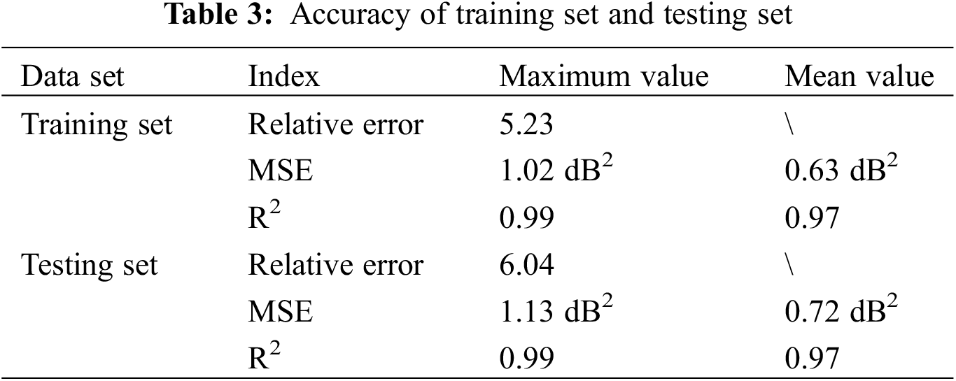
Three evaluation metrics, namely Mean Square Error (MSE), Coefficient of Determination (R2), and Relative error, are used to quantify the model’s prediction results in the frequency domain. MSE and Relative error reflect the gap between the predicted values and the actual values, while the R2 measures the similarity between these values. In general, the closer the MSE and Relative error are to 0, and the closer the R2 is to 1, the higher the prediction accuracy of the model. The corresponding equations are found in Eqs. (10) and (11). From Fig. 13 and Table 2, it can be seen that the prediction accuracy of AE-LSTM is better on a random sample in the test set, and the maximum relative error between the predicted value and the true value in the frequency band of 20–250 Hz is 3.78%., the mean square error is 0.67 dB2, and the R2 is 0.98. Meanwhile, from Fig. 14 and Table 3, it can be seen that the prediction accuracy of AE-LSTM is better in the training and testing sets, and the prediction accuracy of the model in the training set in the frequency band of 20–250 Hz is 3.78%. In the 20–250 Hz frequency band the maximum relative error between the predicted and true values of the training set samples is 5.23%., the maximum MSE is 1.02 dB2, the average MSE is 0.63 dB2, the maximum R2 is 0.99, and the average R2 is 0.97, and similarly, the accuracy of the testing set can be obtained. The accuracy results affirm the feasibility of the established AE-LSTM model for road noise prediction, confirming its effectiveness and high prediction accuracy. It is worth mentioning that AE-LSTM does not appear over-fitting in the prediction process. The reason may be that AE can help extract effective features in the data and remove noise interference, making the data input to the LSTM model more recognizable and robust; through the grid optimization method, the initial learning rate, the number of hidden layer units and the number of epochs of the AE-LSTM model are appropriately adjusted; use a model with appropriate complexity to simplify the network structure as much as possible.

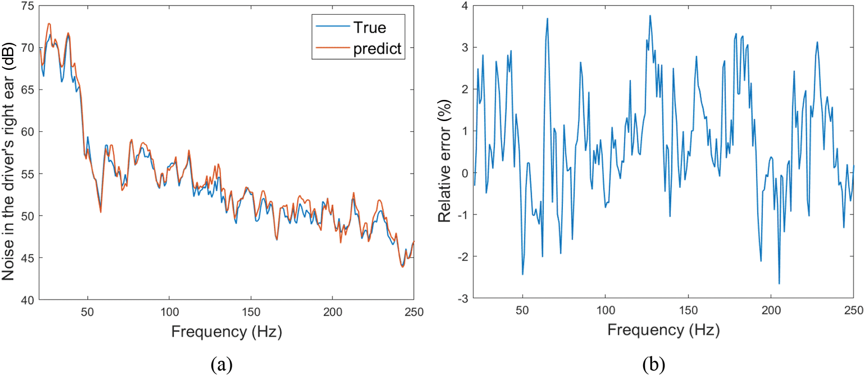
Figure 13: Random sample prediction results. (a) The comparison between the true value and the predicted value. (b) Relative error between true value and predicted value

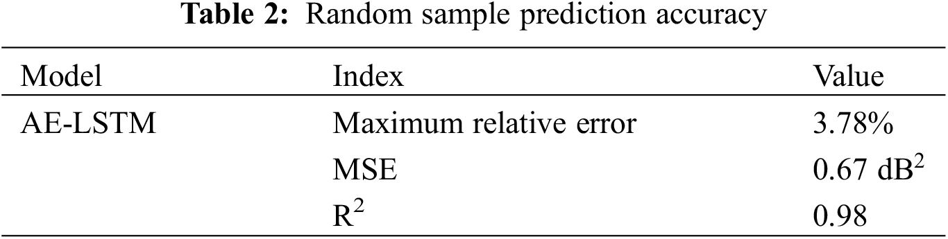
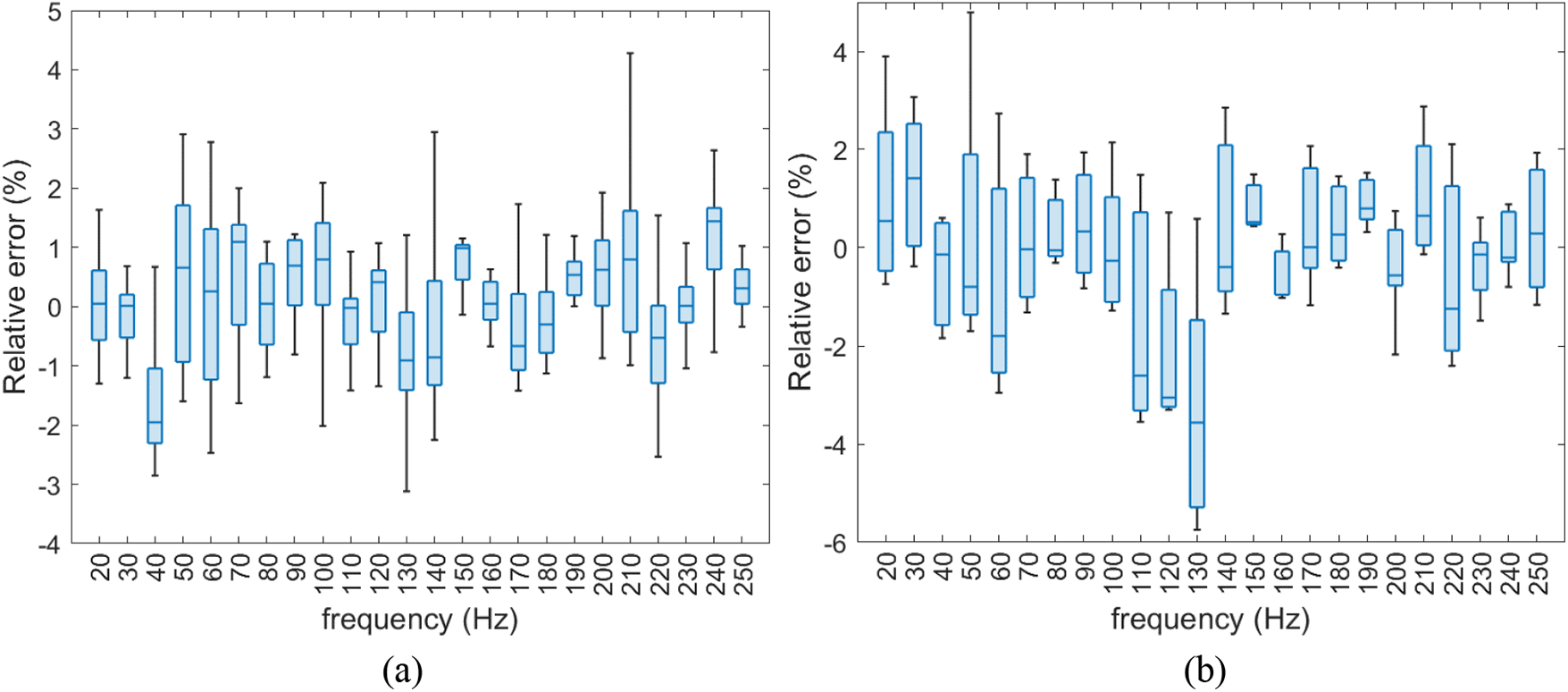
Figure 14: AE-LSTM model training and testing results. (a) Results of the training set. (b) Results of the testing set

MSE=1N∑i=1N⁡(yi−yi~)2 (10)

R2=1−∑i=1N⁡(yi−yi~)2∑i=1N⁡(yi−yi¯)2 (11)

where, N is the sample size, yi represents the true value, yi~ represents the predicted value and yi¯ represents the mean of the true value.

4.3 Comparative Analysis

In order to further verify the high efficiency and high precision of the series model built in this paper, based on the rigid-flexible coupling model and the AE-LSTM prediction model, the full rigid body dynamics model and the full flexible body dynamics model of the vehicle are introduced, as well as Convolutional Neural Network (CNN) and LSTM. MSE, R2 and Relative error are used to test and evaluate the accuracy of noise data prediction of different prediction models and the simulation accuracy of different types of models. At the same time, the efficiency of different neural network models and different dynamic models is evaluated by combining the calculation time. The software used for modeling is MSC Adams2020, MATLAB R2021a, and the computer is configured with 13th Gen Intel (R) Core (TM) i9-13900K processor and 64 GB memory.

Table 4 shows the accuracy and efficiency of the full rigid body model, the rigid-flexible coupling model and the full flexible body model. Among the above models, the full-flexible model has the best accuracy with an MSE of 0.38 × 10−4 m2/s4 and an R2 of 0.83, and the maximal relative errors at 25, 64 and 226 Hz are 6.81%, 8.34% and 9.02%, followed by the rigid-flexible coupling model and the full flexible body model. The corresponding values of each precision index of the rigid-flexible coupling model are 0.42 × 10−4 m2/s4, 0.80, 8.86%., 9.89%. and 9.36%, and the corresponding values of each precision index of the full rigid body model are 0.58 × 10−4 m2/s4, 0.74, 12.36%, 14.51%. and 16.77%. The accuracy difference between the fully flexible model and the rigid-flexible coupling model is small, and the difference of each index is 0.04 × 10−4 m2/s4, 0.03, 2.05%., 1.55%. and 0.34%, respectively. In terms of simulation time, the full rigid body model has the shortest time, followed by the rigid-flexible coupling model, and finally the full flexible body model. The difference between the full flexible body model and the rigid-flexible coupling model is 102.99 s in simulation time. Considering the three factors, the rigid-flexible coupling model performs best in terms of accuracy and efficiency.

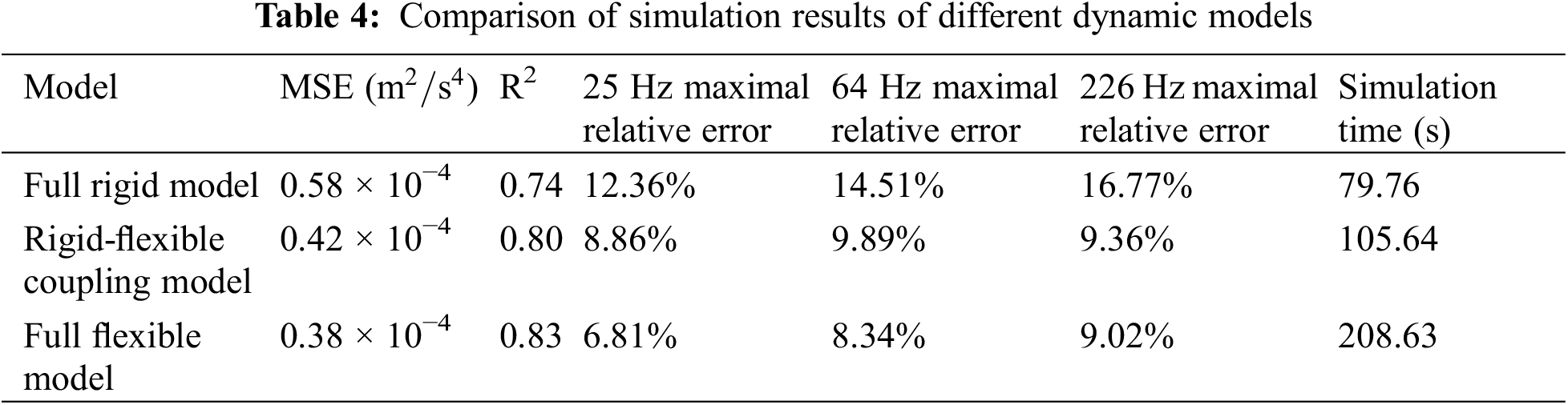
Table 5 and Fig. 15 compare the prediction accuracy and efficiency of CNN model, LSTM model and AE-LSTM model with the simulation results of rigid-flexible coupling model as input data. Among them, the MSE, R2, maximum relative error and training time of the noise prediction results using the CNN model are 4.71 dB2, 0.87, −8.83% and 19.516 s, respectively. The corresponding values of the LSTM model prediction results are 1.15 dB2, 0.95, −6.51%. and 35.667 s, and the corresponding values of the AE-LSTM model prediction results are 0.64 dB2, 0.98, and 3.78%. and 33.478 s. In terms of accuracy, the AE-LSTM model has the highest accuracy, followed by the LSTM model, and finally the CNN model. In terms of training time, the CNN model has the shortest training time, followed by the AE-LSTM model, and the longest LSTM model. The CNN model has poor noise prediction accuracy, but high efficiency. The LSTM model has high accuracy for noise prediction, but low efficiency. The AE-LSTM model has high noise prediction accuracy and high efficiency. Based on the above considerations, the combination of the rigid-flexible coupling model and the AE-LSTM model has high computational efficiency and prediction accuracy, and the effectiveness of the tandem model is verified from the model perspective.

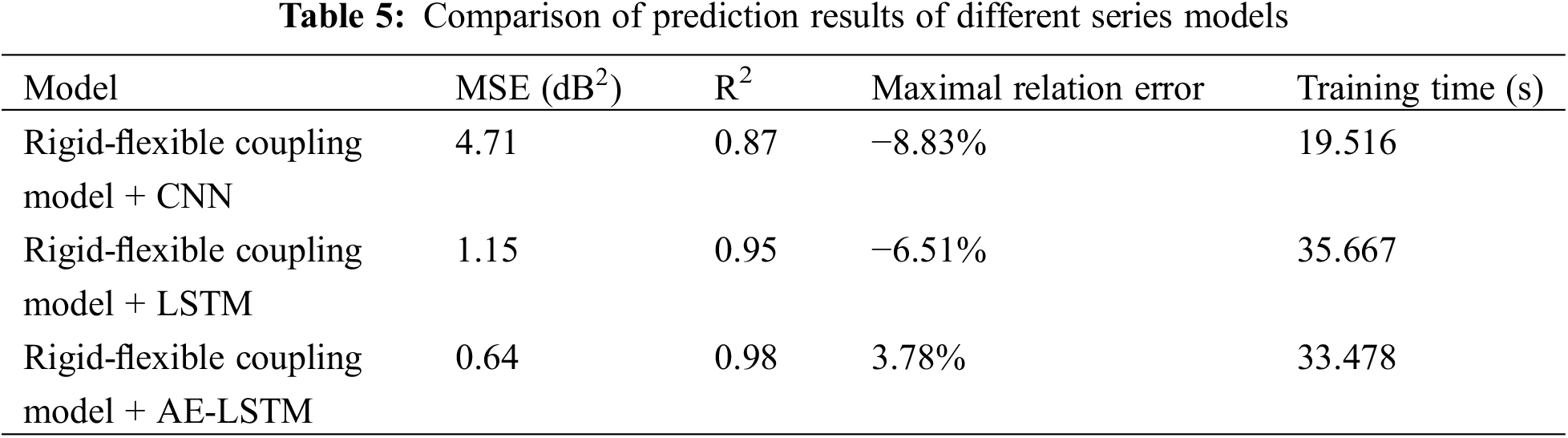
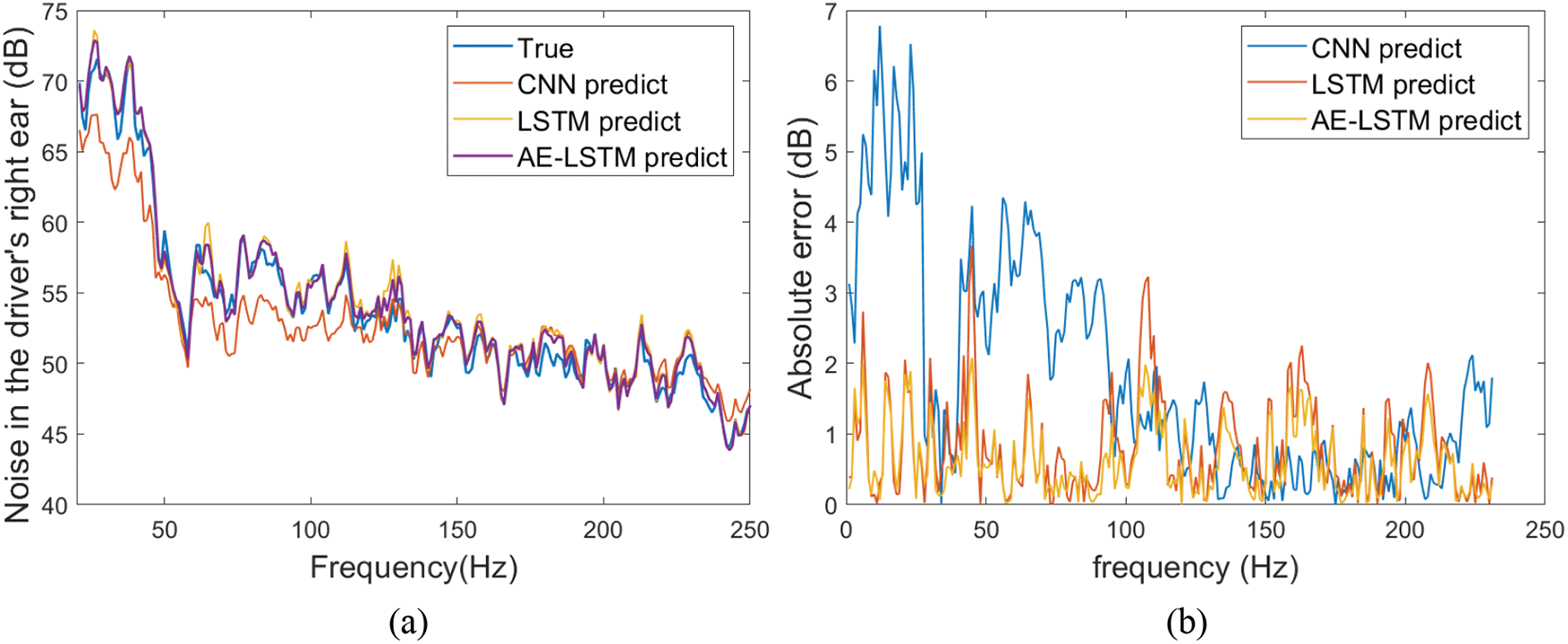
Figure 15: Comparison of prediction results of different models. (a) Comparison of true and predicted values. (b) Relative error between true and predicted values

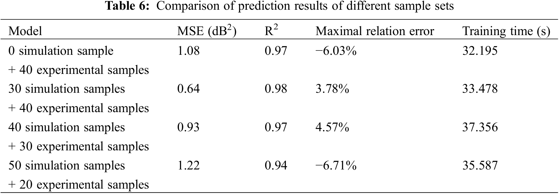
Table 6 shows the comparative analysis of the prediction accuracy and efficiency of the AE-LSTM model against noise when different numbers of simulation samples and test samples of the rigid-flexible coupled model are used as input data. As can be seen from the table, the MSE, R2, maximum relative error and training time are 1.08 dB2, 0.97, −6.03% and 32.195 s when 0 simulation samples and 40 test samples are used as the dataset, and the values are 0.64 dB2, 0.98, 3.78% and 33.478 s when 30 simulation samples and 40 test samples are used as the dataset, respectively. The results show that when the kinetic model simulation results are added to the dataset, the prediction accuracy is greatly improved and has less impact on the efficiency, which affirms that the mechanistic model can effectively solve the problem of data-driven model construction under small sample conditions. Further, when 40 simulation samples and 30 test samples are used as the dataset, the MSE, R2, maximum relative error and training time are 0.93 dB2, 0.97, 4.57% and 37.356 s. When 50 simulation samples and 20 test samples are used as the dataset, the corresponding values are 1.22 dB2, 0.94, −6.71% and 35.587 s. It can be seen that the highest simulation accuracy and efficiency is achieved by using 30 simulation samples and 40 test samples as the data set, followed by 40 simulation samples and 30 test samples as the data set, and the worst is 50 simulation samples and 20 test samples as the data set. It shows that the data quality of the test data is higher than the quality of the simulation data, and the increase of the distribution proportion of the test data can correspondingly improve the accuracy of the network prediction, which affirms the efficiency and accuracy of the series of models from the data perspective.

Based on the above analysis, the following four conclusions can be drawn: (1) the rigid-flexible coupling model has the best performance in terms of accuracy and efficiency; (2) the rigid-flexible coupling model and the AE-LSTM fusion model have higher computational efficiency and prediction accuracy; (3) the mechanism model can effectively solve the problem of constructing the data-driven model under the condition of small samples; (4) the quality of the test data is higher than the quality of the simulation data, and an increase in the distribution ratio of test data can correspondingly improve the accuracy of network prediction. These four conclusions play an important role in proving the superiority of the mechanistic model in tandem with the data-driven model used in the article.

5  Conclusion

In order to overcome the problem that the dynamic model cannot accurately reflect the dynamic characteristics of the vehicle, a rigid-flexible coupling model with dynamic stiffness bushing and flexible components is established. On the basis of this rigid-flexible coupling model, a series model combining mechanism modeling and data-driven modeling is constructed, in which the simulation data of the rigid-flexible coupling model is used as the data source of the data-driven model. In addition, in order to further verify the superiority of the series model constructed in this paper, different types of dynamic models are compared respectively. The results show that the accuracy and efficiency of the rigid-flexible coupling model are better than those of the full rigid body model and the full flexible body model. The MSE, R2, maximum relative error at 25, 64, and 226 Hz and training time are 0.42 × 10−4 m2/s4, 0.80, 8.86%, 9.89%, 9.36% and 105.64 s, respectively. The prediction results of the rigid-flexible coupling model and the series model of different types of data-driven models are compared. The results show that the rigid-flexible coupling model series AE-LSTM has higher accuracy and efficiency, and its MSE, R2, maximum relative error and training time are 0.64 dB2, 0.98, 3.78% and 33.478 s, respectively. The AE-LSTM prediction results with different simulation and test data ratios are compared. The results show that the overall performance of accuracy and efficiency is the best when using 30 sets of simulation samples and 40 sets of test samples as data sets, with values of 0.64 dB2, 0.98, 3.78% and 33.478 s, respectively.

Acknowledgement: The authors would like to acknowledge the support from the Sichuan Provincial Natural Science Foundation and the facilities provided by the Institute of Energy and Power Research at Southwest Jiaotong University for the experimental research.

Funding Statement: This research was funded by the SWJTU Science and Technology Innovation Project, Grant Number 2682022CX008; and the Natural Science Foundation of Sichuan Province, Grant Number 2022NSFSC1892.

Author Contributions: The authors confirm contribution to the paper as follows: conceptualization, methodology: Jian Pang; writing-original draft: Tingting Mao; resources: Wenyu Jia; writing-review and editing: Xiaoli Jia, Peisong Dai; conceptualization, funding acquisition: Haibo Huang.

Availability of Data and Materials: The data used to support the findings of this study are available from the corresponding author upon request.

Conflicts of Interest: The authors declare that they have no conflicts of interest to report regarding the present study.

References

1. Baker, D., Sturesson, P., Sale, C., Kulkarni, K., Boston, C. (2021). Development and optimization of vehicle systems for improved road noise and prediction using vehicle system model in an autonomous vehicle application. SAE International Journal of Advances and Current Practices in Mobility, 4, 299–308. https://doi.org/10.4271/2021-01-1109 [Google Scholar] [CrossRef]

2. Huang, H., Huang, X., Ding, W., Zhang, S., Pang, J. (2023). Optimization of electric vehicle sound package based on LSTM with an adaptive learning rate forest and multiple-level multiple-object method. Mechanical Systems and Signal Processing, 187, 109932. https://doi.org/10.1016/j.ymssp.2022.109932 [Google Scholar] [CrossRef]

3. Huang, H., Huang, X., Ding, W., Yang, M., Yu, X. (2023). Vehicle vibro-acoustical comfort optimization using a multi-objective interval analysis method. Expert Systems with Applications, 213, 119001. https://doi.org/10.1016/j.eswa.2022.119001 [Google Scholar] [CrossRef]

4. Olley, M. (1934). Independent wheel suspension-its whys and wherefors. SAE Journal, 34(3), 73–81. [Google Scholar]

5. Segel, L. (1956). Theoretical prediction and experimental substantiation of the response of the automobile to steering control. Proceedings of the Institution of Mechanical Engineers: Automobile Division, 10(1), 310–330. [Google Scholar]

6. Matschinsky, W. (1987). Die Radführungen der Strassenfahrzeuge. Analyse. In: Synthese, Elasto-Kinematik. Köln: TÜV Rheinland. [Google Scholar]

7. Wang, Y. (2017). Research on key technology of automobile vibration model establishment and verification based on real vehicle driving condition (Master Thesis). Chongqing University of Technology, China. [Google Scholar]

8. Li, F., Li, X., Wo, X., Wen, B. (2021). Analysis and optimization of damping performance of suspension system of hybrid connected vehicle. Journal of Northeastern University (Natural Science Edition), 42(8), 1098–1104 (In Chinese). https://doi.org/10.12068/j.issn.1005-3026.2021.08.006 [Google Scholar] [CrossRef]

9. Hurel, J., Mandow, A., García-Cerezo, A. (2013). Kinematic and dynamic analysis of the MacPherson suspension with a planar quarter-car model. Vehicle System Dynamics, 51(9), 1422–1437. https://doi.org/10.1080/00423114.2013.804937 [Google Scholar] [CrossRef]

10. Fan, D., Dai, P., Yang, M., Jia, W., Jia, X. (2022). Research on maglev vibration isolation technology for vehicle road noise control. SAE International Journal of Vehicle Dynamics, Stability, and NVH, 6, 233–245. https://doi.org/10.4271/10-06-03-0016 [Google Scholar] [CrossRef]

11. Chen, S., Wang, D., Zan, J. (2012). Brake judder analysis using a car rigid-flexible coupling model. Proceedings of the Institution of Mechanical Engineers, Part D: Journal of Automobile Engineering, 226, 348–361. https://doi.org/10.1177/0954407011417760 [Google Scholar] [CrossRef]

12. Chen, S., Shi, T., Wang, D., Chen, J. (2015). Multi-objective optimization of the vehicle ride comfort based on Kriging approximate model and NSGA-II. Journal of Mechanical Science and Technology, 29, 1007–1018. https://doi.org/10.1007/s12206-015-0215-x [Google Scholar] [CrossRef]

13. Chang, H., Gao, Y., Zhang, S. (2023). Load spectrum extraction of double-wishbone independent suspension bracket based on virtual iteration (No. 2023-01-0774). SAE Technical Paper. https://doi.org/10.4271/2023-01-0774 [Google Scholar] [CrossRef]

14. Wang, L., Zhao, Y., Li, L., Ding, Z. (2016). Research on the vibration characteristics of the commercial-vehicle cabin based on experimental design and genetic algorithm. Journal of Vibroengineering, 18(7), 4664–4677. https://doi.org/10.21595/jve.2016.17161 [Google Scholar] [CrossRef]

15. Zeng, Q., Wang, H., Ji, L., Li, S., Huang, Y. (2020). Road noise analysis and optimization research of vehicles based on wheel core loads. Noise and Vibration Control, 40(4), 183–189. https://doi.org/10.3969/j.issn.1006-1355.2020.04.033 [Google Scholar] [CrossRef]

16. Yang, G., Hu, H., Guo, Z., Li, X., Ding, Z. (2015). Load in the NVHD environmen noise performance based on spindle analysis and optimization of vehicle road. 2015 Altair Technology Conference Proceedings, pp. 685–692. Shanghai, China. [Google Scholar]

17. Zou, J., Huss, M., Abid, A., Mohammadi, P., Torkamani, A. et al. (2019). A primer on deep learning in genomics. Nature Genetics, 51(1), 12–18. https://doi.org/10.1038/s41588-018-0295-5 [Google Scholar] [PubMed] [CrossRef]

18. Jayasree, T., Shia, S. (2021). Combined signal processing based techniques and feed forward neural networks for pathological voice detection and classification. Sound & Vibration, 55(2), 141–161. https://doi.org/10.32604/sv.2021.011734 [Google Scholar] [CrossRef]

19. Huang, H., Huang, X., Ding, W., Yang, M., Fan, D. et al. (2022). Uncertainty optimization of pure electric vehicle interior tire/road noise comfort based on data-driven. Mechanical Systems and Signal Processing, 165, 108300. https://doi.org/10.1016/j.ymssp.2021.108300 [Google Scholar] [CrossRef]

20. Lino, M., Fotiadis, S., Bharath, A. A., Cantwell, C. D. (2023). Current and emerging deep-learning methods for the simulation of fluid dynamics. Proceedings of the Royal Society A, 479. https://doi.org/10.1098/rspa.2023.0058 [Google Scholar] [CrossRef]

21. Huang, H., Lim, T. C., Wu, J., Ding, W., Pang, J. (2023). Multitarget prediction and optimization of pure electric vehicle tire/road airborne noise sound quality based on a knowledge- and data-driven method. Mechanical Systems and Signal Processing. https://doi.org/10.1016/j.ymssp.2023.110361 [Google Scholar] [CrossRef]

22. Liu, W., Huang, H., Fan, D., Wang, D., Ding, W. (2023). Vehicle’ s road noise prediction method based on LSTM. Noise and Vibration Control, 61(2), 205–212. https://doi.org/10.3969/j.issn.1006-1355.2023.03.023 [Google Scholar] [CrossRef]

23. Lin, J., Dou, C., Wang, Q. (2018). Comparisons of MFDFA, EMD and WT by neural network, mahalanobis distance and SVM in fault diagnosis of gearboxes. Sound & Vibration, 52(2), 11–15. https://doi.org/10.32604/sv.2018.03653 [Google Scholar] [CrossRef]

24. Wu, Y., Liu, X., Huang, H., Wu, Y., Ding, W. et al. (2023). Multi-objective prediction and optimization of vehicle acoustic package based on ResNet neural network. Sound & Vibration, 57(1), 73–95. https://doi.org/10.32604/sv.2023.044601 [Google Scholar] [CrossRef]

25. Tan, X. (2020). Learn NVH: Noise, vibration, and modal analysis from here. Beijing, China: China Machine Press. [Google Scholar]

26. Koppenaal, J., van Oosten, J., Porsche, I., Chavan, A. (2010). General modeling of nonlinear isolators for vehicle ride studies. SAE International Journal of Materials and Manufacturing, 3(1), 585–591. https://doi.org/10.4271/2010-01-0950 [Google Scholar] [CrossRef]

27. Tian, J. (2020). Simulation analysis and optimization of ride comfort on rigid-flexible coupling vehicle model of heavy tractor, China (Master Thesis). Hefei University of Technology, China. [Google Scholar]

28. Wang, H., Yuan, X., Yang, M. (2019). Network traffic prediction and application based on LSTM and traditional neural networks. Mobile Communications, 43(8), 37–44. https://doi.org/10.3969/j.issn.1006-1010.2019.08.007 [Google Scholar] [CrossRef]

29. Hochreiter, S., Schmidhuber, J. (1997). Long short-term memory. Neural Computation, 9(8), 1735–1780. https://doi.org/10.1162/neco.1997.9.8.1735 [Google Scholar] [PubMed] [CrossRef]

30. Mi, Y., Xu, D., Gao, T. (2023). Application of PCA-LSTM algorithm for financial market stock return prediction and optimization model. International Journal for Simulation and Multidisciplinary Design Optimization, 14, 8. https://doi.org/10.1051/smdo/2023009 [Google Scholar] [CrossRef]

31. Kong, W., Zhang, Y., Jia, Y., Hill, D., Xu, Y. (2017). Short-term residential load forecasting based on LSTM recurrent neural network. IEEE Transactions on Smart Grid, 10(1), 841–851. https://doi.org/10.1109/TSG.2017.2753802 [Google Scholar] [CrossRef]

32. Cheng, J., Dong, L., Lapata, M. (2016). Long short-term memory-networks for machine reading. https://doi.org/10.18653/v1/D16-1053 [Google Scholar] [CrossRef]

33. Ling, Z., Zhang, Y., Cao, G., Chen, J., Li, L. (2022). AE-CNN-based multisource data fusion for gait motion step length estimation. IEEE Sensors Journal, 22(21), 20805–20815. https://doi.org/10.1109/JSEN.2022.3206883 [Google Scholar] [CrossRef]

34. Huang, H., Wu, J., Huang, X., Yang, M., Ding, W. (2020). A generalized inverse cascade method to identify and optimize vehicle interior noise sources. Journal of Sound and Vibration, 467, 115062. https://doi.org/10.1016/j.jsv.2019.115062 [Google Scholar] [CrossRef]

35. Wei, W., Wu, H., Ma, H. (2019). An autoencoder and LSTM-based traffic flow prediction method. Sensors, 19(13), 2946. https://doi.org/10.3390/s19132946 [Google Scholar] [PubMed] [CrossRef]

36. Bates, S., Sienz, J., Langley, D. (2003). Formulation of the Audze-Eglais uniform Latin hypercube design of experiments. Advances in Engineering Software, 34(8), 493–506. https://doi.org/10.1016/S0965-9978(03)00042-5 [Google Scholar] [CrossRef]

37. Syarif, I., Prugel-Bennett, A., Wills, G. (2016). SVM parameter optimization using grid search and genetic algorithm to improve classification performance. TELKOMNIKA (Telecommunication Computing Electronics and Control), 14(4), 1502–1509. https://doi.org/10.12928/telkomnika.v14i4.3956 [Google Scholar] [CrossRef]