HVAC Optimal Control Based on the Sensitivity Analysis: An Improved SA Combination Method Based on a Neural Network

1  Introduction

With the development of economy, increasing energy demand and decreasing supply of fossil fuels, the issue of energy saving becomes more and more important. The “China Building Energy Research Report” in 2017 indicated that China consumed nearly 1 billion tons of standard coal in that year, accounting for about 21% of the country’s energy consumption. The total amount of carbon dioxide emitted has reached about 2 billion tons, accounting for about 19% of the country’s total emissions [1]. More than 30% of global energy consumption is used in buildings [2]. In some other countries and regions, such as Europe, building energy consumption accounts for about 40% of the total energy consumption [3]. In building energy consumption, HVAC systems account for approximately 20% to 50% of total energy consumption [4]. In the United States, HVAC systems account for 41% of primary energy consumption [5]. In India, HVAC systems account for approximately 32% of building energy consumption [6]. HVAC systems are the most commonly used equipment in buildings around the world. By applying an appropriate control strategy, energy efficiency can be effectively improved to optimize system energy consumption [7]. Therefore, the control strategy design of HVAC system, which is one of the systems with the largest energy consumption in buildings, has gradually attracted people’s attention. At the same time, the performance of the HVAC system can be improved through an effective HVAC system control strategy. In general, efficiency can be maximized by adjusting the settings of an HVAC system or subsystem.

In the past two decades, various numerical analysis optimization methods for HVAC systems have been proposed. Newton-Raphson method has the advantages of fewer iterations and fast convergence. Continuously differentiable cost functions can be solved by the interior point method [8]. Branch and Bound method (BaB) describes optimality techniques for discrete systems [9]. Both of these methods can guarantee the optimal solution mathematically.

In addition to numerical analysis optimization methods, HVAC systems can also be optimized using a variety of other methods. Multiplexed optimization schemes are proposed by Sun et al. for complex air conditioning systems [10]. The computational intelligence algorithm proposed in [11] was based on the optimization for HVAC. Using event-driven optimization, Wang et al. proposed a method for controlling HVAC systems instead of using a clock to trigger optimization actions [12,13]. Wang et al. still proposed an event-driven strategy in this field in 2021, a data mining method for optimal control of HVAC systems [14]. The HVAC system has been studied in numerous papers using reinforcement learning, genetic algorithms, ant colony optimization, and deep reinforcement learning [15,16]. There have been many studies of these types in recent years. Chen et al. used Q-Learning to reduce HVAC energy consumption and improve comfort [17]. Berlink et al. proposed a new energy management system RLbEMS based on batch reinforcement learning to reduce power peaks [18]. Wright et al. used a genetic algorithm to better determine the optimal size of HVAC [19]. Srikakulapu et al. used ant colony algorithm to reduce the loss cost of system power [20]. Wang et al. used AC algorithm to optimize the thermal comfort and energy consumption of HVAC and achieved good experimental results [21]. In 2019, Zhang et al. established an HVAC control framework based on the evaluation of dominant actors to simulate and optimize a building energy consumption model [22].

However, most of these optimization algorithms have long optimization training time and heavy computational load [23]. In relevant studies, in a 24-h simulation period, the total time consumed for the genetic algorithm method is 217.6 s when the optimization time interval is 20 min [10]. According to [11], when the optimization time interval is 15 min, the Strength Pareto evolutionary algorithm takes approximately 900 s to calculate. For HVAC systems with online optimal control, these methods take too long to compute. This would result in a degraded optimal control performance because of the long computational time.

Artificial neural networks (ANNs) play an important role in the various optimization methods of HVAC systems [24–27], such as the energy consumption prediction, human thermal comfort measurement, and so on. Atthajariyakul et al. proposed a practical way to quantitatively measure human thermal comfort based on neural computation [26]. Nassif et al. proposed an optimization method for HVAC systems using evolutionary algorithms and artificial neural networks [27]. Afram et al. proposed a new method that used the best network after multiple iterations to improve the prediction performance of ANNs [28]. For HAVC control problems, ANN has attracted too much attention. However, as a black-box model, there are some problems in ANNs, such as slow convergence time and inaccuracy [29].

The main purposes and contributions of this paper are as follows. Firstly, we consider using the SA method to optimize the input of the neural network, which can improve the training efficiency. Secondly, we propose a novel optimization method based on the SA and the trained neural network, which can optimize the control strategy of the HVAC system. Thirdly, we present a set of simulation results of the HAVC system based on the TRNSYS platform, compared with the traditional methods.

2  System Description and Formulation

2.1 Complex AC System

We try to study a commonly used commercial HVAC system that uses all-electric cooling without thermal storage (with primary and secondary chilled water loops). As shown in Fig. 1, there includes cooling towers, chillers, heat exchangers, air-handling units, zones, and air-handling units in a complex HVAC system [30], which can be simulated with the TRNSYS software. These subsystems are verified by the measured data. The heat is dissipated from the cooling towers, chilled water is produced by multiple chillers, while the air-handing units are used to cool the air supply and deliver the regulated air to various areas.

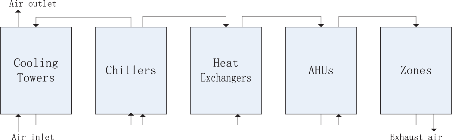
Figure 1: This is a diagram showing the complex system for air conditioning

2.2 System Formulation

In order to optimize the HVAC system, we should clarify the object, such as the objective function and decision factors. The objective function is optimized by adjusting decision factors. In practice, operations or other types of constraints should be taken into account. The optimization algorithm achieves the lowest system energy consumption by minimizing the system power at each point in time, and Eq. (1). Eq. (2) sets out the objectives of minimizing energy consumption of systems.

Psys,tot=Pch,tot+Pct,tot+Ppump,tot+Pfan,tot(1)

(T∗cwT∗chw,prmT∗chw,secT∗sa)=argminTcwTchw,prmTchw,secTsaPsys,tot(2)

where the energy consumption is P subscripted by sys,tot,ch,ct,pump, fan (the system, the chiller, the cooling tower, the pump and the fan); and the temperature is T, subscripted by cw,chw,prm,secandsa, representing the cooling water, the chilled water, the primary, the secondary and the air supply respectively; in each superscript “*”, we have listed the optimum value for the corresponding decision factor.

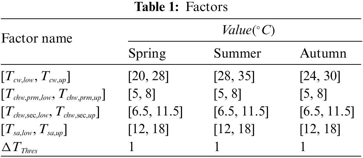
According to [30], they are the temperature of cooling water supply (CWS), cooling water supply in heat exchangers, chilled water supply in cooling towers and the temperature of air supply. There is a strong relationship between these factors and the energy consumption of the HVAC system. In addition, the study found that the optimal state values of these variables are not fixed, but also change according to the system operation [10]. The total power of the system can be regarded as a function of these four factors. Eqs. (3)–(8) are constraints. The minimum and maximum points set by these four factors are subject to Eqs. (3)–(6). Moreover, two additional constraints are represented in Eqs. (7) and (8). Eq. (7) represents the maximum temperature difference, which cannot be larger than the threshold (for example 1°C), to prevent the set point from changing too much, resulting in the system instability. The purpose of Eq. (8) is to ensure that the primary and secondary chilled water loops have minimal temperature differences. Table 1 lists the exact settings.

Tcw,low≤Tcw≤Tcw,up(3)

Tchw,prm,low≤Tchw,prm≤Tchw,prm,up(4)

Tchw,sec,low≤Tchw,sec≤Tchw,sec,up(5)

Tsa,low≤Tsa≤Tsa,up(6)

|Te(k+1)−Tek|≤ΔTThres(7)

Tchw,prm,e+ΔTmin≤ΔTchw,sec,e(8)

3  Sensitivity Analysis Combination Method

3.1 Sensitivity Analysis Method

In sensitivity analysis, we examine how the uncertainty associated with one or more input variables can affect the output variables. This method improves or model predictions by qualitatively and/or quantitatively studying the way the model responds to changes in variables, and by analyzing the interactions between variables to understand the phenomenon in question.

The perturbation technique is used to analyze the sensitivity of factors in HVAC systems, and a total of 6 perturbation actions, {0.3, −0.2, −0.1, 0.1, 0.2, 0.3}(ΔT), are adopted to analyze the relevant factors (T), such as cooling water supply temperature (Tcw), chilled water supply temperature (Tchw), chilled water supply temperature in heat exchangers (Tchw_HX) and supply air temperature (Tsa). These factors are used to analyze the sensitivity, which are called decision factors. In the analysis process, 10 initial states (representing the above four factors) are selected. And at each time, only one factor is perturbed, and get the difference value (ΔP) between the obtained energy consumption and the initial energy consumption (P). The ratio of the relative changes is ΔT/TΔP/P, which is used to represent the sensitivity of the T on the P. During the sensitivity analysis, Simlab software assists in verifying the result.

The two factors, which have an important impact on energy consumption, are called sensitivity factors, and another two factors, which have a little impact on energy consumption, are called non-sensitivity factors.

3.2 Neural Networks Construction Based on Sensitivity Analysis Method

There are three factors associated with HVAC system optimization problems: the non-control factor, the continuous control factor, and the discrete control factor. Non-controlled factors can be measured and affect energy consumption, but may not be controlled. Typical non-controlled factors in the HVAC system are wet bulb temperature, dry bulb temperature, and cooling load. Continuous control factors and discrete control factors are related to the set value and operation mode of energy consumption minimization. Combined with three factors and the relevant field knowledge, the candidate factors are normal solar flux, infrared radiation, outdoor temperature, wind speed, cooling water supply temperature, chilled water temperature, calculate the temperature of the supply air, the cooling load, and the temperature of the dry and wet bulbs. Among these factors, some of them are redundant and not even about energy consumption. Therefore, the selection of appropriate factors can not only reduce the number of model training, but also improve the model accuracy.

This paper considered the sensitivity analysis, and the reliability and robustness of data. In such a case, the temperature of the supply water used for cooling, the temperature of chilled water used for cooling in the heat exchangers, the temperature of supply air delivered to the heat exchanger, the cooling load, the temperature of dry bulbs, and the temperature of wet bulbs were selected as the inputs of the network. During the same time period, the number of neurons in the input layer of the factor changed proportionately, as shown by the sensitivity analysis results. For example, as the sensitivity analysis results of Tcw, Tchw, Tchw_HX, and Tsa were a, b, c, and d adjust to the number of neurons of these four factors in the input layer according to the ratio (a:b:c:d).

3.3 Sensitivity Analysis Combination Method

In this paper, an optimization algorithm, named Sensitivity Analysis Combination Method (SAC), is presented to optimize the energy consumption of HVAC systems. All subsystems interact with each other. If one subsystem’s energy consumption is reduced, another subsystem’s energy consumption may increase. Therefore, all of the decision factors in HVAC systems are taken into account for sensitivity analyses. As shown in Fig. 2.

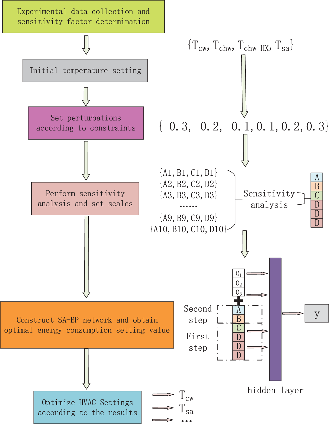
Figure 2: SAC for HVAC system applications

According to the sensitivity analysis, the four factors are divided into sensitivity factors and non-sensitivity factors. Therefore, the optimal value of the minimum energy consumption of the sensitivity factor is considered firstly, and then, the optimal value of the minimum energy consumption of the non-sensitive factor is considered. The details are as follows:

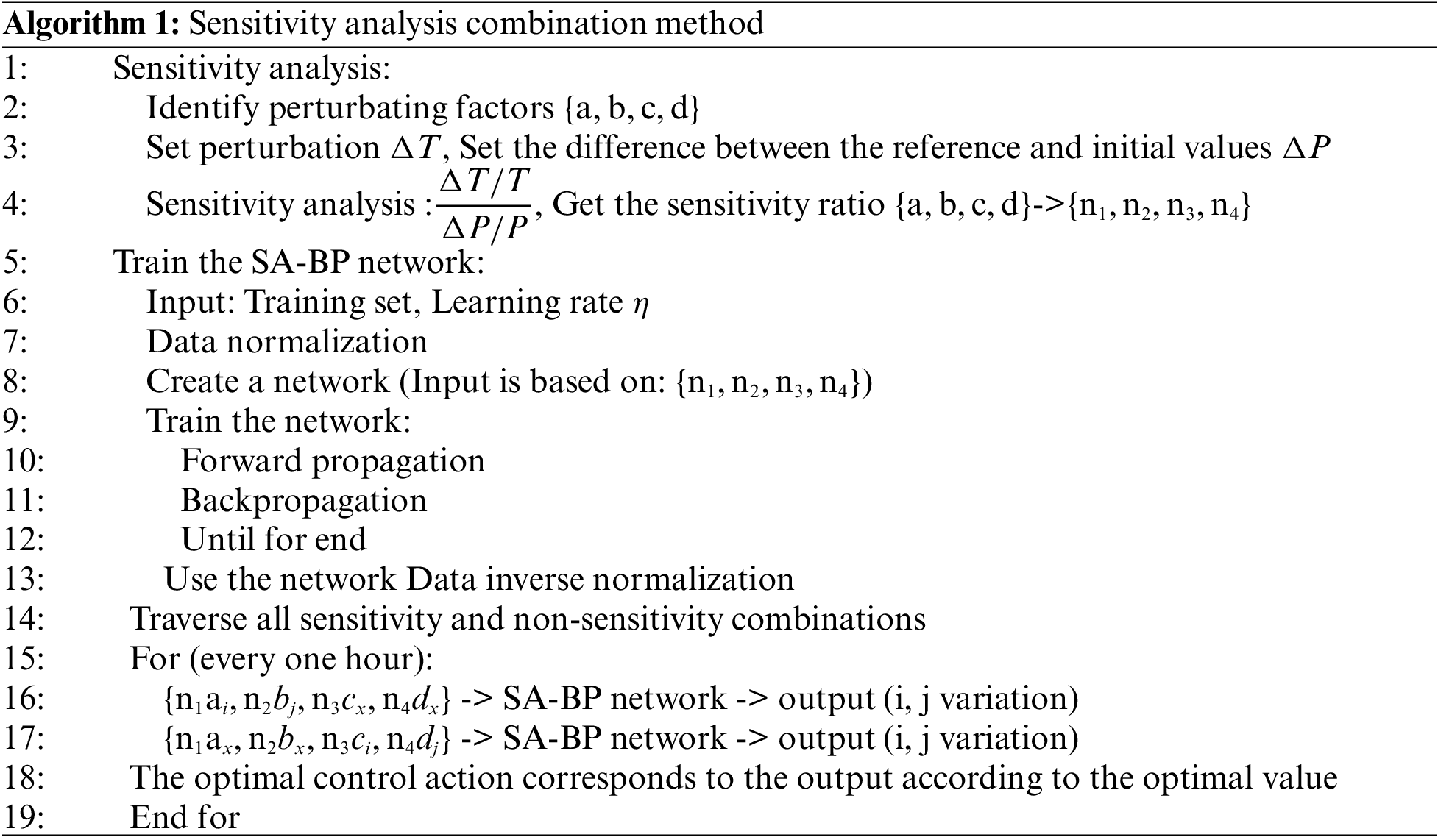
Because of the constraint of Eqs. (7) and (8), the four decision factors’ controllable space is divided by 0.1, so the controllable space of each decision factor has 21 regions, resulting in 441 combinations of two sensitivity factors and 882 combinations of SAC. Firstly, the combination of sensitivity factors is used to obtain the energy consumption prediction by the trained neural network (non-sensitive factors value is unchanged), and then all the energy consumption prediction is traversed. The optimization value is assigned to sensitivity factors. Secondly, non-sensitive factors are combined to obtain the energy consumption prediction by the trained neural network (sensitivity factors value is new). Then, traverse all the energy consumption prediction, and finally, a setting value for optimal energy consumption is obtained. According to this optimal value, the HVAC system optimizes the cooling water temperature, supply air temperature and other related Settings. The specific process is shown in Algorithm 1.

:

4  Analysis of Experimental Results

4.1 SAC

4.1.1 Data Collection

To train a better neural network, the bigger the data set is, the better performance the neural network does. The training data set comes from two parts: one comes from the collected data, and the other comes from the system simulation (generated from the HVAC simulation model constructed by TRANSYS platform). Using a mixture of 2 parts of the data set, can effectively reduce the data loss caused by simulation error.

Considering cooling load, dry bulb temperature, wet bulb temperature variation (see Appendix A for the detailed value), and the time lag in the system, the energy consumption model is constructed over a time interval of 1-h in this study. During each optimization stage (every 60 min), setpoints for the cooling water supply temperature, chilled water temperature, chilled water temperature in the heat exchanger, and supply air temperature are randomly selected. The data is recorded every minute for 6 days. Two parts of the data are randomly mixed, of which 75% is used to train the model and 25% is used for testing.

4.1.2 Sensitivity Analysis

The sensitivity analysis results of Tcw, Tchw, Tchw_HX and Tsa are shown in Table 2, which used the methods in Section 3.1. Tchw_HX and Tsa, called sensitivity factors, have a great influence on the energy consumption. Meanwhile, Tcw and Tchw, called non- Sensitivity factors, have less influence.

The sensitivity analysis results are verified by the Simlab software. Firstly, by setting the range of values of Tcw, Tchw, Tchw_HX and Tsa, 1000 sets of state combinations are generated by the Simlab software. The 1000 sets of state set values are put into the simulation model separately in the same external environment, the energy consumption generated is obtained. The energy consumption value is input into the Simlab software, thereby obtaining a sensitivity analysis map. The results verify Tchw_HX and Tsa are highly sensitive to the energy consumption, while Tcw and Tchw are less sensitive to the energy consumption.

4.1.3 Sensitivity Analysis Construct the Neural Network

There are three layers in a traditional neural network, the input layer, the hidden layer and the output layer. When constructing the neural network, connections between the data are often overlooked. The normalization method used by traditional neural networks can avoid numerical problems and speed up neural network learning, while data normalization also weakened the importance of the sensitive data in input and output data. Therefore, this paper uses the sensitivity analysis based on the input layer data, and considers to increase the number of the input layer for sensitivity factors.

The neural network constructed in this paper is firstly based on the BP propagation algorithm, which is a feedforward neural network trained by back-propagating errors. The training of the BP algorithm includes forward propagation to obtain the error and back propagation of the error. When the error is not within a satisfactory range, the back propagation of the error will be carried out until it stops. The back propagation of the error is to divide the error into each layer unit to correct the weight. The neural network is divided into three layers, taking the hidden layer as the input to the output layer as an example. As in Eq. (9), E is the total output error, where pi is the predicted value, yi is the output value, and i corresponds to the corresponding output layer unit. Eq. (10) represents the derivative relationship between the total error and the current hidden layer unit. Eq. (11) is the sum of the input of the i-th output unit, Eq. (12) is the derivative relationship between the total error and the output of each unit, which k corresponds to the k-th hidden layer unit, and wki is the weight between the corresponding two units. value. The same theory applies between the hidden layer and the input layer, so that the weights of each unit can be updated.

E=12∑i=1n(pi−yi)2(9)

∂E∂zi=∂E∂pi∂pi∂zi=(pi−yi)pi(1−pi)(10)

zi=∑k=1npk′wki(11)

∂E∂pk′=∑i=1n∂E∂ziwki=∑i=1n(pi−yi)pi(1−pi)wki(12)

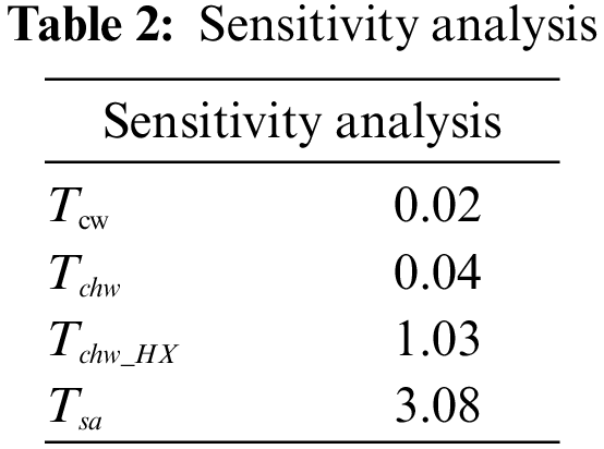
According to the sensitivity analysis results in Table 2, the sensitivity analysis back propagation (SA-BP) neural network constructed in this paper contains 9 neurons in the input layer, which corresponded to 1 neuron in cold load, 1 neuron in dry bulb temperature, and 1 neuron in wet bulb temperature. Tcw is 1 neuron, Tchw is 1 neuron, Tchw_HX is 1 neuron, Tsa is 3 neurons. The input layer data is [cold load, dry bulb, wet bulb, Tcw, Tchw, Tchw_HX, Tsa, Tsa, Tsa]. The hidden layer contains 40 neurons and the output layer has one neuron. The network structure of SA-BP is shown in Fig. 3.

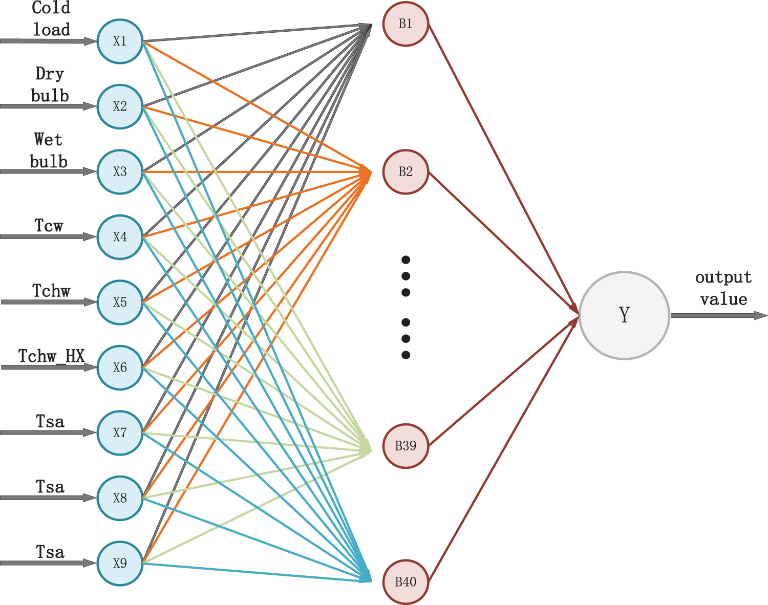
Figure 3: SA-BP network structure diagram

We will carry out two-part operations. First, traverse 441 combinations of sensitivity factors at intervals of 0.1, and input them to Tchw_HX  and Tsa  in Fig. 3, and output to find the optimal energy consumption value. The second step is to traverse 441 combinations of insensitive factors with Tchw_HX  and Tsa  unchanged, and input them to Tcw  and Tchw  in Fig. 3. Further find out the optimal energy consumption value.

The SA-BP neural network is compared with the back propagation (BP) neural network. The convergence results are shown in Fig. 4. Due to the randomness of weight initialization, three experiments were conducted, and the convergence times of the BP neural network were 370, 332, and 417, and the mean was about 373. The number of convergence times of the SA-BP neural network is 123, 91, and 136, and the mean is about 117. It can be clearly seen from the average that the convergence rate of the SA-BP algorithm is faster, much faster than that of ordinary BP neural network structures. Twenty samples were randomly selected from the test set. The accuracy analysis is shown in Fig. 5. where y-bp and y-sabp are the predicted value obtained from the model, while y is the actual value measured. It can be clearly seen that under normal circumstances, the deviation between the energy consumption value predicted by SA-BP and the real value is smaller than the deviation between the energy consumption value predicted by BP and the real value. The experiment compares the average of 20 results of the two methods and finds that the average error of the BP neural network is 77, and the average error of the SA-BP neural network is 36. On the basis of the sensitivity analysis, it can be seen that the neural network constructed is higher in comparison to the other methods in terms of convergence speed and accuracy.

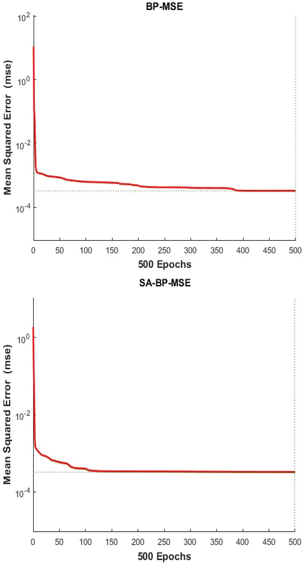
Figure 4: Convergence analysis of BP and SA-BP

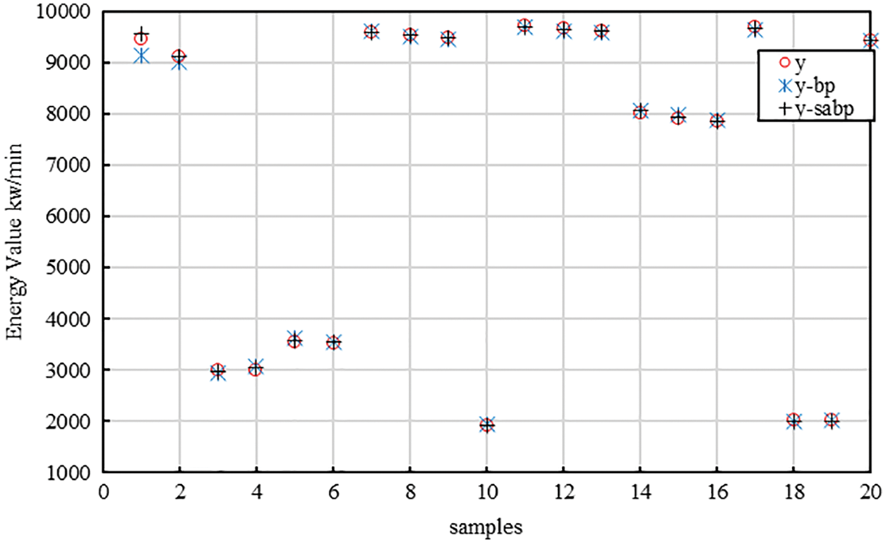
Figure 5: Neural network accuracy analysis of BP and SA-BP

4.1.4 System Optimization

The sensitivity analysis results in Table 2 show that Tchw_HX and Tsa are sensitivity factors, Tcw and Tchw are non-sensitivity factors. Firstly, Tchw_HX and Tsa are combined for consideration, when Tcw and Tchw remain unchanged, all the predicted energy consumption of SA-BP combination is traversed. The value of the lowest predicted energy consumption is assigned to Tchw_HX and Tsa. Then, Tcw and Tchw are combined for consideration, all the predicted energy consumption of combination by SA-BP is traversed. The value of the lowest predicted energy consumption is assigned to Tcw and Tchw. Finally, we can determine the value of four factor.

4.2 Other Methods

Exhaustive methods (EXM) are a kind of classical optimization method, that enumerate all the possible situations of a certain problem. There are four decision factors in this experiment, namely Tchw_HX, Tsa, Tcw, Tchw, which is governed by the stability of the HVAC system (each decision factor should ideally not change more than one degree), and is limited by the response time of the HVAC system (when the range of each decision factor is large, long search time). The simulation crashed because the set value could not be retrieved in time. As such, each decision factor has a range of [−0.5°C to + 0.5°C] (T is its initial value). To satisfy the constraint, the range should be truncated if it exceeds Eqs. (7) and (8). We formed 14641 states based on the four decision factors, and we then used a trained neural network to predict the energy consumption for each state. Lastly, choose the point that consumes the least energy.

Random search method (RS) is a kind of simple method, which tries to find the optimal solution in the solution space by randomness. According to the law of big numbers, if the number of random points is big enough, it can get the optimal solution. The experiment divided into 4 decision factors: Tchw_HX, Tsa, Tcw, Tchw, taking into account the stability of the HVAC system (the maximum change value for each factor should be within 1 degree), and the HVAC system The system response time is limited, so the factor range for each decision factor is set to [T−1°C, T+1°C] (T is the initial level of each factor). To satisfy the constraint, the range should be truncated when it exceeds Eqs. (7) and (8). Therefore, the four decision factors can construct 194481 states. The method selects 5000 points in the accepted region randomly, then uses the trained neural network to obtain the predicted results of energy consumption. Next, the neural network is applied in order to obtain predictions of energy consumption for the state. The last step is to select the point with the lowest consumption of energy.

4.3 Results and Analysis

Three experiments were conducted, one in spring, one in summer, and one in autumn. A combination of all three optimization methods, including the cooling load, dry bulb temperature, wet bulb temperature, cooling water supply temperature, chilled water supply temperature, chilled water supply temperature in the heat exchangers, and air temperature setting, is optimized at each optimization stage (every 60 min). Depending on which method is used to optimize the cooling water supply temperature, the chilled water supply temperature, the chilled water supply temperature in the exchangers, as well as the supply air temperature, the various values are determined on the control devices. The performance of all three methods was simulated and evaluated using two indicators: the daily energy consumption and the computational load, where energy performance is represented by the first indicator, and computational complexity is represented by the second indicator.

4.3.1 Energy Performance Comparison

Comparing the algorithm to the benchmark case, the energy performance was evaluated. Various decision factors were set as constants, including the cooling water supply temperature, the chilled water supply temperature, the chilled water supply temperature in the heat exchangers, and the supply air temperature. The benchmark settings are shown in Table 3.

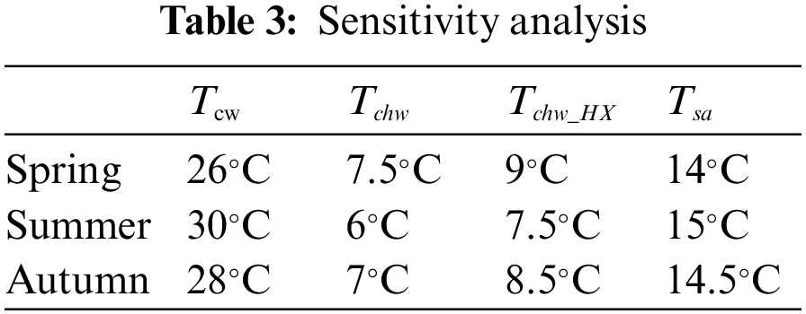
The Figs. 6–8 show the energy saving effect of EXM, RS, and SAC compared with the benchmark. Most of the time, the energy consumption of HVAC system of RS is much higher, while EXM and SAC can achieve similar lower energy consumption of HVAC system. EXM which is limited by the search space has higher energy consumption than SAC. Furthermore. As shown in Table 4, these methods produce different energy conversation rates each day in spring, summer, and autumn. From the Table 4, for all three seasons, SAC has the highest daily energy saving rate.

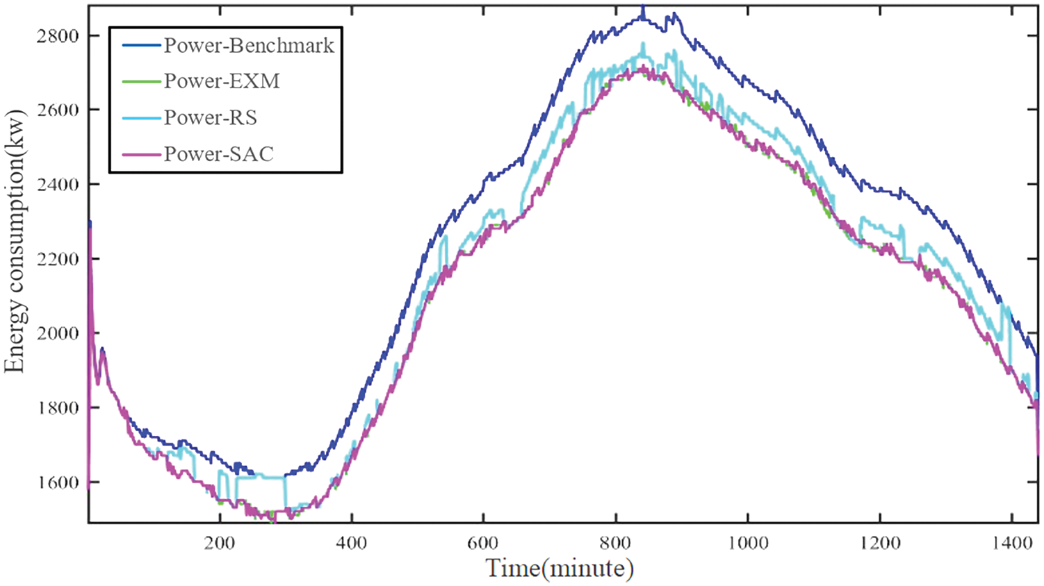
Figure 6: The energy consumption of a spring day

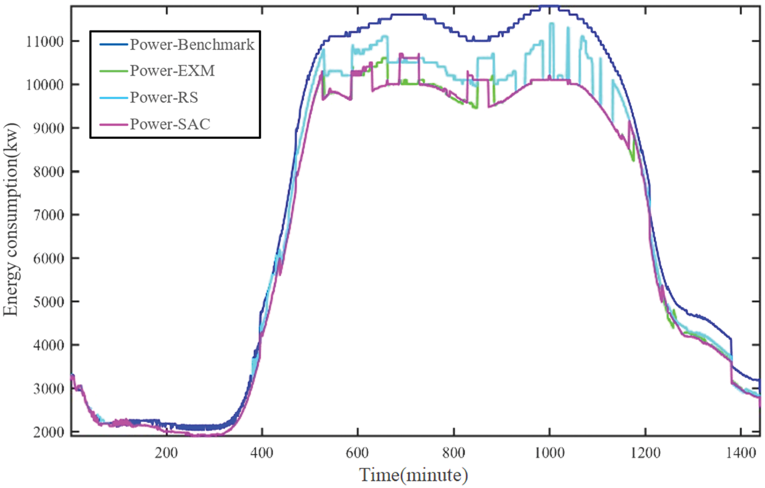
Figure 7: The energy consumption of a summer day

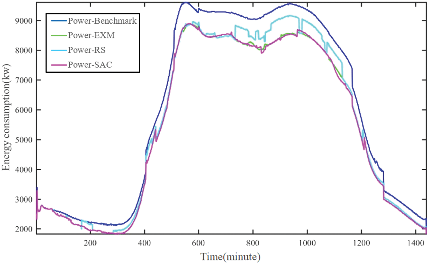
Figure 8: The energy consumption of an autumn day

4.3.2 Calculation Load Comparison

Table 5 compared the computational load of EXM, RS, and SAC. The calculation amount was the time required for the optimization method to search for the optimal setting. The calculations of each algorithm simulate the running load of one day, and EXM was used as a benchmark for calculating the load comparison. It can be seen that RS reduces the computational load compared to the baseline, saving 64.1%, 64.7%, and 64.3% in spring, summer, and autumn respectively. At the same time, SAC significantly reduces the computational load compared to the baseline, saving 91.3%, 91.2%, and 91.8% in spring, summer, and autumn respectively. In a word, SAC has the lowest load calculation than others in three seasons.

5  Conclusion

In this paper, the main contributions to energy consumption optimization of HVAC systems are as follows:

We proposed a new sensitivity analysis combination method (SAC) for energy conversion optimization in HVAC systems. On this basis, the neural network is optimized, and then the relevant settings of the HVAC system are optimized, including cooling water temperature, chilled water temperature and supply air temperature. Based on the data of existing HVAC systems, various optimization control methods were tested and evaluated on TRNSYS simulation HVAC systems. The results show that SAC and EXM can find lower energy consumption points in the two-month simulation experiment. RS and SAC can obtain set points in a short time. Therefore, according to the experimental results, the SAC designed by us performs better in terms of energy savings and computational time.

In future work, two points for improvement will be considered. The first one is to consider whether there is a better optimization method for sensitivity analysis than the analysis method used in this paper. The second one is to use more effective methods to replace the existing ergodic sensitivity combination methods. Moreover, some more advanced and effective fuzzy control methods may have better results. For example, in future work, we will try to use Type-3 Logic Fuzzy system to solve the energy consumption optimization of HVAC system, which is a kind of fractional-order multi-model Type-3 fuzzy control for nonlinear systems with unmodeled dynamics and has achieved some good control performance in related fields, such as model on solar panels problem. We believe that using a more scientific and intelligent method to optimize the energy consumption of HVAC energy consumption is a very meaningful research field in the future.

Funding Statement: This work was financially supported by National Key R&D Program of China (No. 2020YFC2006602), National Natural Science Foundation of China (Nos. 62072324, 61876217, 61876121, 61772357), University Natural Science Foundation of Jiangsu Province (No. 21KJA520005), Primary Research and Development Plan of Jiangsu Province (No. BE2020026).

Conflicts of Interest: The authors declare that they have no conflicts of interest to report regarding the present study.

References

1. Meng, D., Wu, L. (2020). Forecasting the building energy consumption in China using grey model. Environmental Processes, 7(3), 1009–1022. https://doi.org/10.1007/s40710-020-00438-3 [Google Scholar] [CrossRef]

2. Sharif, S. A., Hammad, A. (2019). Developing surrogate ANN for selecting near-optimal building energy renovation methods considering energy consumption, LCC and LCA. Journal of Building Engineering, 25, 100790. https://doi.org/10.1016/j.jobe.2019.100790 [Google Scholar] [CrossRef]

3. Alcala, R., Jm, B., Casillas, J., Cordon, O., Perez, R. (2003). Fuzzy control of hvac systems optimized by genetic algorithms. Applied Intelligence, 18, 155–177. https://doi.org/10.1023/A:1021986309149 [Google Scholar] [CrossRef]

4. Pérez-Lombard, l., Ortiz, J., Pout, C. (2008). A review on buildings energy consumption information. Energy & Buildings, 40(3), 394–398. https://doi.org/10.1016/j.enbuild.2007.03.007 [Google Scholar] [CrossRef]

5. Afram, A., Janabi-Sharifi, F. (2014). Theory and applications of HVAC control systems–A review of model predictive control (MPC). Building and Environment, 72, 343–355. https://doi.org/10.1016/j.buildenv.2013.11.016 [Google Scholar] [CrossRef]

6. Vakiloroaya, V., Samali, B., Fakhar, A., Pishghadam, K. (2014). A review of different strategies for HVAC energy saving. Energy Conversion and Management, 77, 738–754. https://doi.org/10.1016/j.enconman.2013.10.023 [Google Scholar] [CrossRef]

7. Du, Y., Zandi, H., Kotevska, O., Kurte, K., Munk, J. et al. (2020). Intelligent multi-zone residential HVAC control strategy based on deep reinforcement learning. Applied Energy, 281(1). https://doi.org/10.1016/j.apenergy.2020.116117 [Google Scholar] [CrossRef]

8. Kusiak, A., Xu, G., Zhang, Z. (2014). Minimization of energy consumption in HVAC systems with data-driven models and an interior-point method. Energy Conversion and Management, 85, 146–153. https://doi.org/10.1016/j.enconman.2014.05.053 [Google Scholar] [CrossRef]

9. Ferreira, P. M., Ruano, A. E., Silva, S., Conceicao, E. Z. E. (2012). Neural networks based predictive control for thermal comfort and energy savings in public buildings. Energy and Buildings, 55, 238–251. https://doi.org/10.1016/j.enbuild.2012.08.002 [Google Scholar] [CrossRef]

10. Sun, Y., Huang, G., Li, Z., Wang, S. (2013). Multiplexed optimization for complex air conditioning systems. Building & Environment, 65, 99–108. https://doi.org/10.1016/j.buildenv.2013.03.024 [Google Scholar] [CrossRef]

11. He, X., Zhang, Z., Kusiak, A. (2014). Performance optimization of HVAC systems with computational intelligence algorithms. Energy and Buildings, 81, 371–380. https://doi.org/10.1016/j.enbuild.2014.06.021 [Google Scholar] [CrossRef]

12. Wang, J., Jia, Q. S., Huang, G., Sun, Y. (2018). Event-driven optimal control of central air-conditioning systems: Event-space establishment. Science and Technology for the Built Environment, 24(8), 839–849. https://doi.org/10.1080/23744731.2018.1457410 [Google Scholar] [CrossRef]

13. Wang, J., Liu, R., Zhang, L., Asad, H. S., Meng, E. (2019). Triggering optimal control of air conditioning systems by event-driven mechanism: Comparing direct and indirect approaches. Energies, 12(20), 3863. https://doi.org/10.3390/en12203863 [Google Scholar] [CrossRef]

14. Wang, J., Hou, J., Chen, J., Fu, Q., Huang, G. (2021). Data mining approach for improving the optimal control of hvac systems: An event-driven strategy. Journal of Building Engineering, 39, 102246. https://doi.org/10.1016/j.jobe.2021.102246 [Google Scholar] [CrossRef]

15. Fu, Q., Han, Z., Chen, J., Lu, Y., Wu, H. et al. (2022). Applications of reinforcement learning for building energy efficiency control: A review. Journal of Building Engineering, 50(104165), 1–22. https://doi.org/10.1016/j.jobe.2022.104165 [Google Scholar] [CrossRef]

16. Ahn, K. U., Park, C. S. (2019). Application of deep Q-networks for model-free optimal control balancing between different HVAC systems. Science and Technology for the Built Environment, 26(1), 61–74. https://doi.org/10.1080/23744731.2019.1680234 [Google Scholar] [CrossRef]

17. Chen, Y., Norford, L. K., Samuelson, H. W., Malkawi, A. (2018). Optimal control of HVAC and window systems for natural ventilation through reinforcement learning. Energy and Buildings, 169, 195–205. https://doi.org/10.1016/j.enbuild.2018.03.051 [Google Scholar] [CrossRef]

18. Berlink, H., Costa, A. H. (2015). Batch reinforcement learning for smart home energy management. IJCAI’15: Proceedings of the 24th International Conference on Artificial Intelligence, pp. 2561–2567. Argentina. [Google Scholar]

19. Wright, J. A. (1996). HVAC optimisation studies: Sizing by genetic algorithm. Building Services Engineering Research and Technology, 17(1), 7–14. https://doi.org/10.1177/014362449601700102 [Google Scholar] [CrossRef]

20. Srikakulapu, R., Vinatha, U. (2018). Optimized design of collector topology for offshore wind farm based on ant colony optimization with multiple travelling salesman problem. Journal of Modern Power Systems and Clean Energy, 6(6), 1181–1192. https://doi.org/10.1007/s40565-018-0386-4 [Google Scholar] [CrossRef]

21. Wang, Y., Velswamy, K., Huang, B. (2017). A long-short term memory recurrent neural network based reinforcement learning controller for office heating ventilation and air conditioning systems. Processes, 5, 46–63. [Google Scholar]

22. Zhang, Z., Chong, A., Pan, Y., Zhang, C., Lam, K. P. (2019). Whole building energy model for hvac optimal control: A practical framework based on deep reinforcement learning. Energy and Buildings, 199, 472–490. https://doi.org/10.1016/j.enbuild.2019.07.029 [Google Scholar] [CrossRef]

23. Wu, Z., Karimi, H. R., Dang, C. (2019). An approximation algorithm for graph partitioning via deterministic annealing neural network. Neural Networks, 117, 191–200. https://doi.org/10.1016/j.neunet.2019.05.010 [Google Scholar] [PubMed] [CrossRef]

24. Jiang, B., Wu, Z., Karimi, H. R. (2022). A distributed dynamic event-triggered mechanism to HMM-based observer design for H∞ sliding mode control of Markov jump systems. Automatica, 142, 110357. https://doi.org/10.1016/j.automatica.2022.110357 [Google Scholar] [CrossRef]

25. Wu, Z., Karimi, H. R., Dang, C. (2019). A deterministic annealing neural network algorithm for the minimum concave cost transportation problem. IEEE Transactions on Neural Networks and Learning Systems, 31(10), 4354–4366. https://doi.org/10.1109/TNNLS.2019.2955137 [Google Scholar] [PubMed] [CrossRef]

26. Atthajariyakul, S., Leephakpreeda, T. (2005). Neural computing thermal comfort index for HVAC systems. Energy Conversion and Management, 46(15–16), 2553–2565. https://doi.org/10.1016/j.enconman.2004.12.007 [Google Scholar] [CrossRef]

27. Nassif, N. (2014). Modeling and optimization of HVAC systems using artificial neural network and genetic algorithm. Building Simulation, 7(3), 237–245. https://doi.org/10.1007/s12273-013-0138-3 [Google Scholar] [CrossRef]

28. Afram, A., Janabi-Sharifi, F., Fung, A. S., Raahemifar, K. (2017). Artificial neural network (ANN) based model predictive control (MPC) and optimization of HVAC systems: A state of the art review and case study of a residential HVAC system. Energy and Buildings, 141, 96–113. https://doi.org/10.1016/j.enbuild.2017.02.012 [Google Scholar] [CrossRef]

29. Wu, Z., Gao, Q., Jiang, B., Karimi, H. R. (2021). Solving the production transportation problem via a deterministic annealing neural network method. Applied Mathematics and Computation, 411, 126518. https://doi.org/10.1016/j.amc.2021.126518 [Google Scholar] [CrossRef]

30. Wang, J., Huang, G., Sun, Y., Liu, X. (2016). Event-driven optimization of complex HVAC systems. Energy and Buildings, 133, 79–87. https://doi.org/10.1016/j.enbuild.2016.09.049 [Google Scholar] [CrossRef]

Appendix A

A.1 load and weather data

The cooling load profile of 3 days in 2013 was adopted as the relevant cooling load factors. In 2013, April, August, and October correspond to the typical spring, summer, and autumn. The profiles were measured in a high-rise building in Hong Kong. The measurement results are that the building has a maximum cooling load of 5940 kW in spring, while it has a maximum cooling load of 20,800 kW in summer; and in the autumn, 14,500 kW reached its peak. In the spring, the cooling load was 4598 kW, in the summer it was 14,959 kW, and in the autumn, it was 10,038 kW [1]. Figs. A1–A3 show the distribution of cooling loads over three days, and Figs. A1–A3 depict the daily weather profiles from Hong Kong Observatory for those three days at the same time.

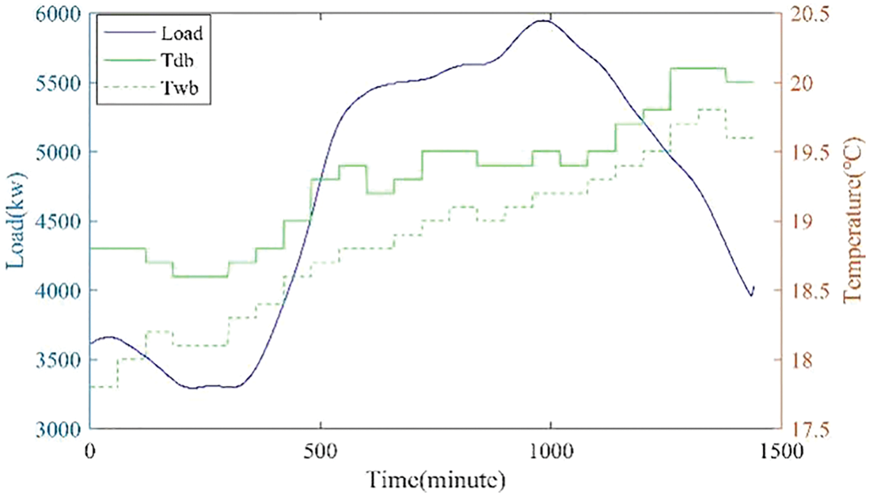
Figure A1: The load profile of a spring day

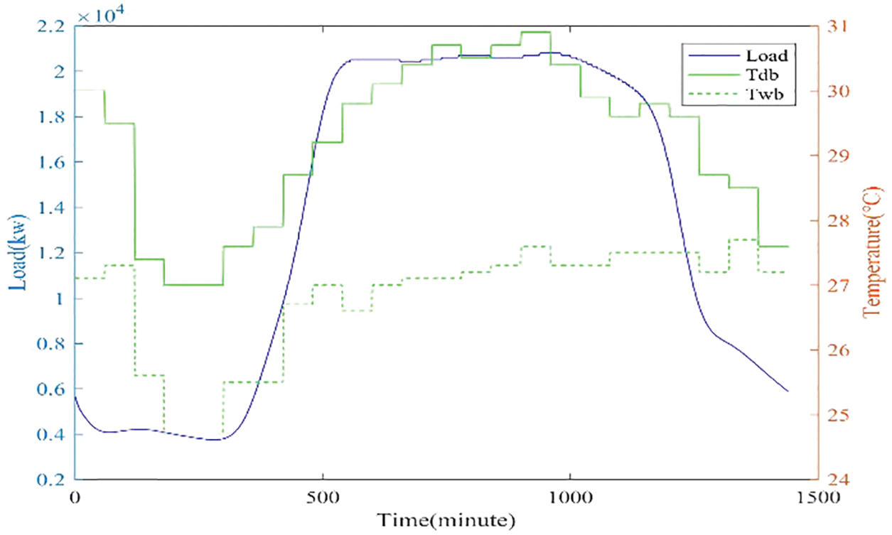
Figure A2: The load profile of a summer day

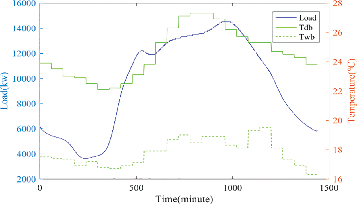
Figure A3: The load profile of an autumn day