A Survey on Artificial Intelligence in Posture Recognition

1  Introduction

In recent years, posture recognition has been a research hotspot in computer vision and artificial intelligence (AI) [1], which analyzes the original information of the target object captured by a sensor device or camera through a series of algorithms to obtain the posture. Human body posture recognition has broad market prospects in many application fields, such as behavior recognition, gait analysis, games, animation, augmented reality, rehabilitation testing, sports science, etc. [2]. AI-based posture recognition has also attracted more and more attention from researchers. We retrieved literature on AI-based posture recognition every year from 2000 to 2022, and the number of them showed an increasing trend, as shown in Fig. 1.

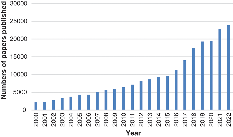
Figure 1: The number of posture recognition papers published (2000–2022)

Although human posture recognition has become the leading research direction in the field of posture recognition, there are also many studies on animal posture recognition, such as birds [3], pigs [4,5], and cattle [6]. With the rise of artificial intelligence, more and more scholars are interested in the research of posture recognition.

According to the input image type, we generally divide posture recognition algorithms into two categories: algorithms based on RGB images and algorithms based on depth images. The RGB image-based recognition algorithm utilizes the contour features of the human body. For example, the edge of the human body can be described through the histogram of oriented gradients (HOG). The depth-based image algorithm mainly uses the image’s gray value to represent the target’s spatial position and contour. The latter is not disturbed by light, color, shadow, and clothing, but it has higher requirements for information image acquisition equipment [7,8].

The existing posture recognition methods can be summarized into two methods. One is based on the traditional machine learning method, and the other is based on the deep neural network method. In the posture recognition method based on traditional machine learning, the traditional image segmentation algorithm is introduced to realize the segmentation of an image or action video. Then machine learning methods are used for classification, such as support vector machines (SVM), Gaussian mixture model (GMM), and hidden Markov models (HMM). The disadvantage of this method is that the representation ability of these features is limited, representative semantic information is challenging to extract from complex content, and step-by-step recognition lacks good real-time performance.

In the recognition method based on deep learning, the low level-feature information of the image is combined with the deep neural network to estimate and recognize the posture at a higher level. Compared with traditional machine learning algorithms, target detection networks based on deep neural networks often have stronger adaptability and can achieve higher recognition speed and accuracy [9].

We conducted a systematic review based on the Preferred Reporting Items for Systematic Review and Meta-Analysis (PRISMA). Through Google scholar, Elsevier, and Springer Link, we searched the papers on the application of artificial intelligence to posture recognition. According to the title and content, we eliminated irrelevant and duplicate papers, and finally, the review included 188 papers. The PRISMA chart is shown in Fig. 2.

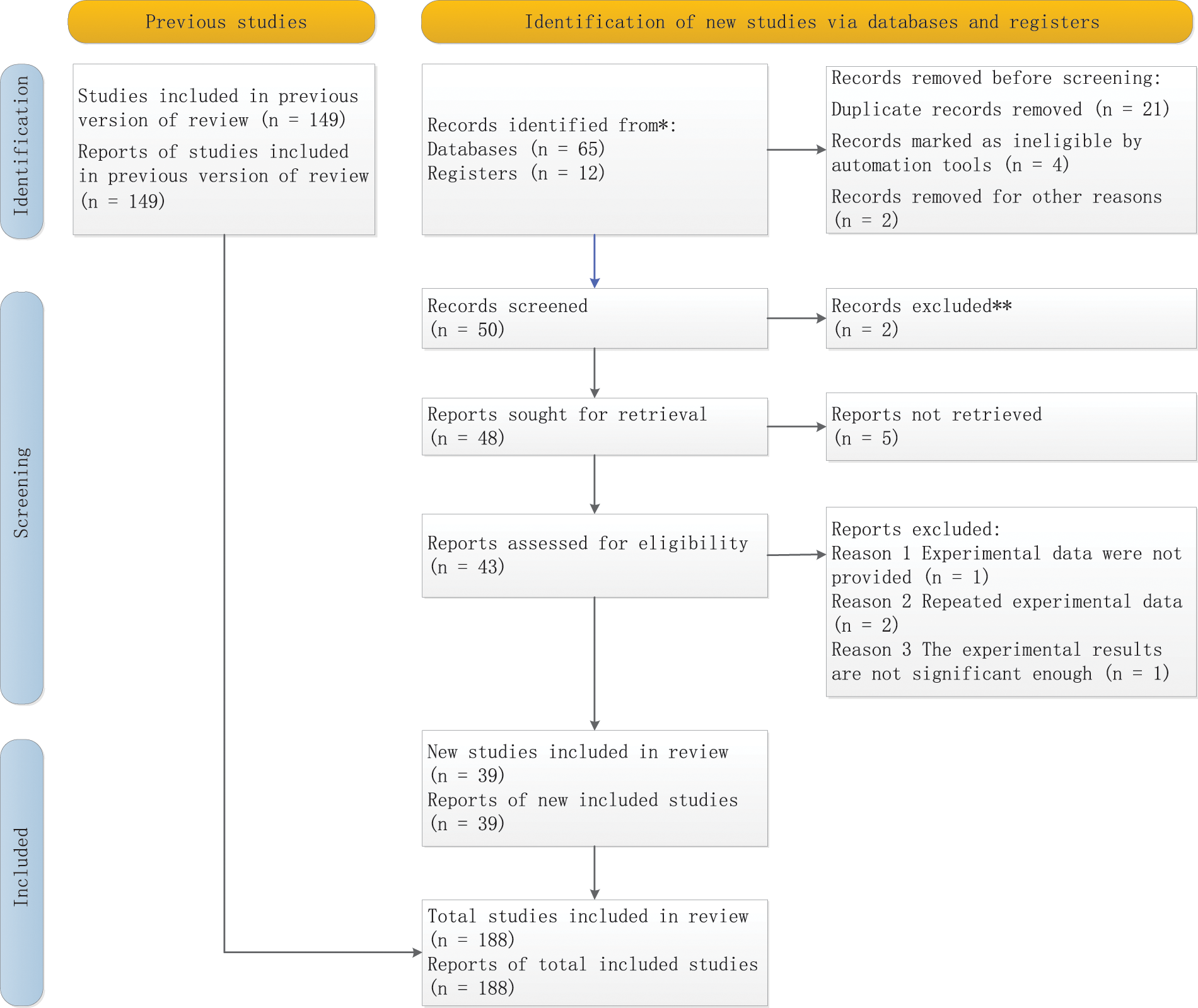
Figure 2: The PRISMA chart of the article selection process for this review

2  Main Recognition Techniques

2.1 Sensor‑Based Recognition

The sensor-based posture recognition requires the target to wear a variety of sensors or optical symbols and collect the action information of the target object based on this. The research on sensor-based human posture recognition algorithms started earlier. As early as the 1950s, some people used gravity sensors to recognize human posture [10]. In daily human posture recognition research, sensors have been used to distinguish standing, walking, running, sitting, and other stable human posture [11,12].

The common classification methods of posture recognition sensors are as follows. According to the position of the sensor, it can be divided into lower limbs, waist, arm, neck, wrist, etc. Sensors can also be classified according to the number of sensors, which can be divided into single-sensor and multi-sensor. Compared with the method of single-sensor signal processing, the multi-sensor system can obtain more information about the measured target and environment effectively [13,14].

Whether or not the sensor is installed on the user can be divided into wearable and fixed sensors. Wearable devices are a representative example of sensor-based human activity recognition (HAR) [15,16]. The sensor’s type of data output can be divided into array time domain signal, image matrix data, vector data, or strap-down matrix data. Common wearable sensors include inertial sensors (such as accelerometers and gyroscopes), physiological sensors (such as EEG, ECG, GSR, EMG), pressure sensors (such as FSR, bending sensors, barometric pressure sensors, textile-based capacitive pressure sensors), vision wearable sensors (such as WVS), flexible sensors [17].

To avoid physical discomfort and system instability caused by workers on construction sites wearing invasive sensors or attaching multiple sensors to the body, Antwi-Afari et al. [18] utilized the network based on deep learning as well as wearable insole sensor data to automatically identify and classify various postures presented by workers during construction. Hong et al. [19] designed a system using multi-sensors and a collaborative AI-IoT-based approach and proposed multi-pose recognition (MPR) and cascade-adaboosting-cart (CACT) posture recognition algorithms to further improve the effect of human posture recognition.

Fan et al. [20] proposed a squeezed convolutional gated attention (SCGA) model to recognize basketball shooting postures fused by various sensors. Sardar et al. [21] proposed a mobile sensor-based human physical activity recognition platform for COVID-19-related physical activity recognition, such as hand washing, hand disinfection, nose-eye contact, and handshake, as well as contact tracing, to minimize the spread of COVID-19.

2.2 Vision‑Based Recognition

The vision-based method extracts the information of the key node and skeleton by analyzing the position of each joint point of the target object in the image data. In vision-based methods, cameras are usually used to obtain images or videos that require posture recognition and can be used in a non-contact environment. Therefore, this method does not affect the comfort of motion and has low acquisition costs.

Obtaining human skeleton keypoints from two-dimensional (2D) images or depth images through posture estimation is the basis of vision-based posture recognition. There are inherent limitations when 2D images are used to model three-dimensional (3D) postures, so RGB-D-based methods are ineffective in practical applications. In addition to RGB images and depth maps, skeletons have become a widely used data modality for posture recognition, where skeleton data are used to construct high-level features that characterize 3D configurations of postures [22].

The general process of vision-based posture recognition includes the following: image data acquisition, preprocessing, feature extraction, and feature classification, as shown in Fig. 3.

Figure 3: Procedure of vision-based posture recognition

Currently, video-based methods mainly use deep neural networks to learn relevant features from video images for posture recognition directly. For example, WMS Abedi et al. [23] used convolutional neural networks to identify and classify different categories of human poses (such as sitting, lying, and standing) in the available frames. Tome et al. [24] fused the probabilistic information of 3D human posture with the multi-stage CNN architecture to achieve 3D posture estimation of the original images. Fang et al. [25] designed a visual teleoperation framework based on a deep neural network structure and posture mapping method. They applied a multi-level network structure to increase the flexibility of visual teleoperation network training and use. Kumar et al. [26] used the integration of six independent deep neural architectures based on genetic algorithms to improve the driver’s performance on the distraction classification problem to assist the existing driver-to-pose recognition technology. Mehrizi et al. [27] proposed a computer vision-based label-free motion capture method that combines the discriminative method of posture estimation with morphological constraints to improve the accuracy and robustness of posture estimation.

2.3 RF-Based Recognition

In some specific posture recognition situations, the target object cannot wear the sensing device, and radio frequency (RF)-based technology can solve this problem. Due to their non-contact nature, various radio frequency-based technologies are finding applications in human activity recognition. Yao et al. [28] used radio frequency identification (RFID) technology to build a posture recognition system to identify the posture of the elderly, who do not need to wear equipment at this time. Yao et al. [29] used RFID and machine learning algorithms to decipher signal fluctuations to identify activities. Liu et al. [30] proposed a sleep monitoring system based on passive RFID tags, which combined hierarchical recognition, image processing, and polynomial fitting to identify body posture through changes caused by backscattered signals from tags.

Radio frequency signals are extremely sensitive to environmental changes, and changes caused by human movements or activities can be easily captured. Radio frequency signals are absorbed, reflected, and scattered by the body, which will cause changes in the signals. Human activities will cause different changes in the radio frequency signal so that human activities can be identified by analyzing the changes in the signals. The most typically used radio frequency technologies are radar, WiFi, and RFID [31,32].

3  Traditional Machine Learning‑Based Approach

3.1 Preprocessing

Image preprocessing is the basis of posture recognition, which can directly affect the extraction of feature points and the result of posture classification, thus affecting the recognition rate of posture. The main tasks in the preprocessing stage are denoising, human skeleton keypoint detection, scale, gray level normalization, and image segmentation.

The keypoint detection of the human skeleton mainly detects the keypoint information such as human joints and facial features. The output is the skeletal feature of the human body, which is the primary part of posture recognition and behavior analysis, mainly used for segmentation and alignment.

The normalization of scale and gray level should first ensure the effective extraction of key features of the human body and then process the color information and size of the image to reduce the amount of computation.

3.2 Feature Extraction

3.2.1 Figure Format Histogram of Oriented Gradients

Histogram of oriented gradient (HOG) constitutes features by calculating and statistical histogram of gradient direction in local image regions [33], which describes the entire image region and reflects strong description ability and robustness. HOG classifier is generally combined with the SVM classifier in image recognition, especially in human detection, which has achieved great success. HOG can describe objects’ appearance features and the shape of local gradient distribution [34]. HOG feature extraction steps are as follows in Fig. 4.

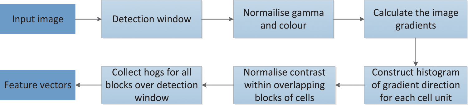
Figure 4: The flowchart of HOG feature extraction

(1) The color space of input images is normalized by gamma correction to reduce the influence of light factors and suppress noise interference. Gamma compression is shown in the following formula:

I(a,b)=I(a,b)γ.(1)

Here, the value of gamma has three conditions:

(i) When gamma is equal to 1, the output value is equal to the input value, and only the original image will be displayed.

(ii) When gamma is greater than 1, the dynamic range of the low gray value region of the input image becomes smaller, and the contrast of the low gray value region of the image is reduced. In the area of high gray value, as the dynamic range increases, the contrast in the area of high gray value of the image will be correspondingly enhanced. Eventually, the overall gray value of the image will be darkened.

(iii) When gamma is less than 1, the dynamic range of the low gray value region of the input image becomes larger, and the contrast of the low gray value region of the image is enhanced. In the area of high gray value, if the dynamic range becomes smaller, the contrast in the area of high gray value will decrease accordingly, thus brightening the overall gray level of the image.

(2) The horizontal and vertical gradient values and the gradient direction values of each pixel in the image can be calculated by the following formula:

Ga(a,b)=H(a+1,b)−H(a−1,b),(2)

Gb(a,b)=H(a,b+1)−H(a,b−1),(3)

where Ga(a,b) represents the horizontal gradient, Gb(a,b) represents the vertical gradient, and H(a,b) represents the pixel value at pixel point (a, b).

The gradient amplitude and orientation at the pixel point are shown in Eqs. (4) and (5), respectively:

G(a,b)=Ga(a,b)2+Gb(a,b)2,(4)

α(a,b)=arctan⁡Gb(a,b)Ga(a,b).(5)

(3) The gradient orientation histogram is constructed for each cell unit to provide the corresponding code for the local image region. At the same time, the image of the human posture and appearance are kept weak sensitivity.

(4) Every few cell units are formed into large blocks, and the gradient intensity is normalized to realize the compression of illumination, shadow, and edge.

(5) All overlapping blocks in the detection window are collected for HOG features and combined into the final feature vector for classification.

3.2.2 Scale‑Invariant Feature Transform

Scale Invariant Feature Transform (SIFT) is an algorithm that maps images to local feature vector sets based on computer vision technology. The essence is to find the keypoints or feature points in different scale-spaces and then calculate the direction of the keypoints [35].

Therefore, SIFT features do not vary with the changes in image rotation, scaling, and brightness and are almost immune to illumination, affine transformation, and noise [36]. Yang et al. [37] used SIFT feature extraction to study writing posture and achieved good results. The main steps of SIFT algorithm are as follows in Fig. 5.

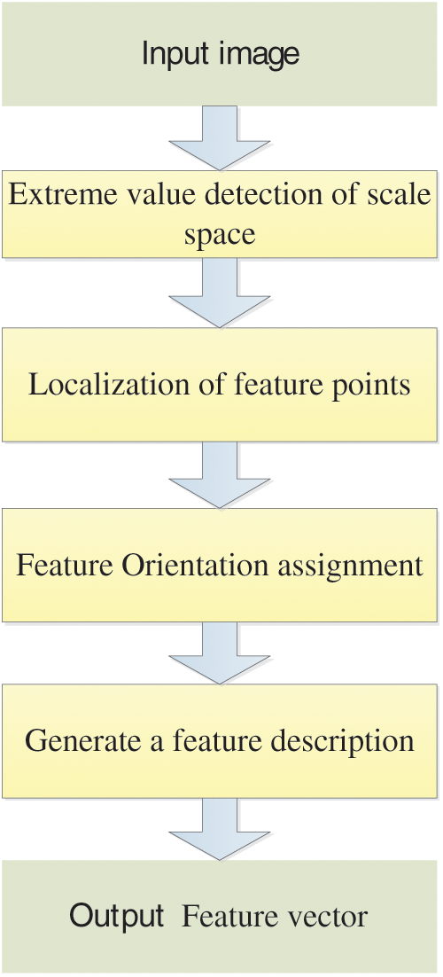
Figure 5: The flowchart of SIFT algorithm

(1) Extreme value detection of scale space

Images over all scale spaces are searched, and Gaussian differential functions are used to identify potential points of interest that are not affected by scale and selection. This can be done efficiently by using the “scale space” function as follows:

G(x,y,δ)=12πδ2ex2+y22δ2,(6)

S(x,y,δ)=G(x,y,δ)×I(x,y),(7)

where G(x,y,δ) is a Gaussian kernel function, (x,y) is the space coordinate, δ refers to the scale space factor, and S(x,y,δ) refers to the Gaussian scale space of the image. The purpose of establishing the scale space is to detect the feature points that exist on different scales. The Gaussian Laplacian operator (LoG) is a good operator for detecting feature points, but its computation is extremely large, so the Gaussian difference (DoG) is usually used to approximate LoG.

D(x,y,δ)=S(x,y,kδ)−S(x,y,δ).(8)

Here, k is the scaling factor of two adjacent Gaussian scale spaces.

(2) Localization of feature points

At this stage, we need to remove the points that do not meet the criteria from the list of keypoints. The points that do not meet the requirements are mainly low-contrast feature points and unstable edge response points.

(3) Feature orientation assignment

One or more directions should be assigned to each keypoint location according to the local gradient direction of the image to achieve rotation invariance. To ensure the invariance of these features, scholars perform all subsequent operations on the orientation, scale, and position of the keypoints. After finding the feature point, the scale of the feature point and its scale image can be obtained:

h(x,y)=(L(x+1,y)−L(x−1,y))2+(L(x,y+1)−L(x,y−1))2,(9)

θ(x,y)=arctan⁡L(x,y+1)−L(x,y−1)L(x+1,y)−L(x−1,y).(10)

Here, h(x,y) and θ(x,y) denote the magnitude and orientation of the gradient at each point L(x,y), respectively. After calculating the gradient direction, the gradient orientation and amplitude of the pixel near the feature point are calculated by the histogram.

In the histogram, the horizontal axis represents the intersection angle of the gradient orientation, the vertical axis represents the sum of the gradient amplitudes corresponding to the gradient orientation, and the orientation corresponding to the peak value is the primary orientation of the feature points.

(4) Generate a feature description

After the above operation, the feature point descriptor must be generated, containing the feature points and the pixels around them. In general, the generation of feature descriptors consists of the following steps: (i) To achieve rotation invariance, the main orientation of rotation is corrected. (ii) Generate descriptors and form 128-dimensional feature vectors. (iii) Normalize the feature vector length to remove illumination’s influence.

3.2.3 Dynamic Time Warping

In time series analysis, dynamic time warping (DTW) is introduced to compare the similarity or distance between two arrays or time series of different lengths. DTW was initially used in speech recognition and is now widely used in posture recognition [38–41].

Suppose there are two sequences denoted by P=[P1,P2,…,Pm] and Q=[Q1,Q2,…,Qn]. Here, m and n are the lengths of the two sequences, respectively. When m is equal to n, the Euclidean distance (formula (11)) can be directly used to calculate the distance d between the two sequences.

d=∑i=1m(Pi−Qi)2.(11)

When m is not equal to n, DTW is introduced to regularize the sequence to make it matches. To align the two sequences, construct a matrix grid of m × n. The elements in the matrix (a, b) are the distance between Pi and Qi, that is, the similarity between each point in sequence P and each point in sequence Q. The smaller the distance, the higher the similarity, and the shortest path from the start to the end. This path is called the “warping path” and is denoted by W. The lth element of W is defined as:

Wl=(a,b)l,(12)

W=w1,w2,…,wl,…,wL,max(m,n)≤L<m+n−1.(13)

This path needs to satisfy the following constraints [42]:

(1) The order of each sequence part cannot be changed, and the selected path starts at the bottom left corner of the matrix and ends at the top right corner. The boundary conditions must be met, as shown in Eq. (14):

{w1=(1,1)wL=(m,n)(14)

(2) Ensure that each coordinate in the two sequences appears in the warping path W, so a point can only be aligned with its neighboring point.

(3) The points above the warping path W must be monotonically progressed over time.

Therefore, only three directions to choose the path to each grid point. Assuming the path has already passed through grid point (a, b), the location of the next grid point to pass through can only be one of three cases: (a + 1, b), (a, b + 1), and (a + 1, b + 1), as shown in Fig. 6. We can solve the value of DTW according to Eq. (15).

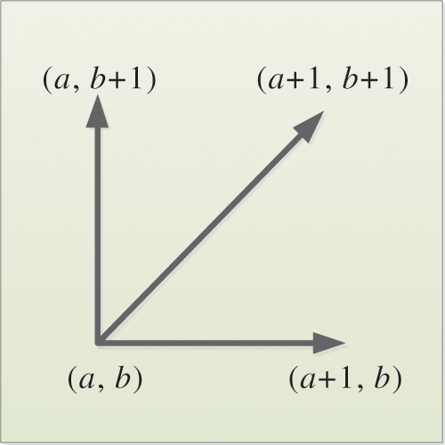
Figure 6: Diagram of the path search direction

DTW(P,Q)=min{∑l=1LwlL}.(15)

3.2.4 Other Feature Extraction Approaches

In addition to the above two feature extraction methods (HOG [43–46], SIFT [47–49], DTW [50,41,39,40]) for posture recognition, several feature extraction methods are widely used in posture recognition, such as Hu moment invariant (HMI) [51,52], Fourier descriptors (FD) [53,54], nonparametric weighted feature extraction (NWFE) [55,56], gray-level co-occurrence matrix (GLCM) [57,58].

3.3 Feature Reduction

After feature extraction is completed, feature dimension reduction is needed when the dimension is too high to improve the speed and efficiency of calculation and decision-making. Principal component analysis (PCA) [59] and linear discriminant analysis (LDA) [60] are the most commonly used dimensionality reduction methods.

PCA aims to try to recombine the numerous original indicators with certain correlations into a new set of unrelated comprehensive indicators and then replace the original ones [61]. It is an unsupervised dimensionality reduction algorithm. LDA is a supervised linear dimensionality reduction algorithm. Unlike PCA, LDA maintains data information and makes dimensionality reduction data as easy to distinguish as possible [62].

3.4 Classification

3.4.1 SVM

Corinna Cortes et al. first proposed the support vector machine (SVM) to find the optimal solution from two types of different sample data [63]. There may be multiple partition hyperplanes for the sample space to separate the two training samples. SVM is used to find the best hyperplane to separate the training samples.

Therefore, the main idea of the support vector machine is to establish a decision hyperplane and realize the division of two different types of samples by obtaining the maximum distance between two types of samples closest to the plane on both sides of the plane [9], as shown in Fig. 7. Here, Vij indicates the support vector, and all of which are divided into two categories by the hyperplane.

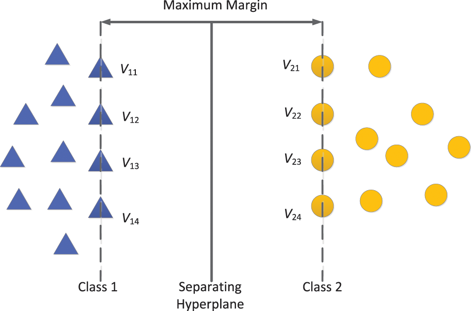
Figure 7: Schematic diagram of linear support vector machine

The model trained by SVM is only related to the support vector, so the algorithm’s complexity is mainly affected by the number of support vectors. Vectors and labels can define the training samples in the two-dimensional feature space. The N training samples in the m-dimensional feature space are defined as:

{(Xi,yi)}i=1N,(16)

Xi=[xi1xi2⋮xim],yi∈{1,−1}.(17)

Here, Xi indicates the ith vector of the sample space, yi indicates the category of the ith sample. If the training sample is linearly separable, we describe the hyperplane by the following equation [64]:

wT⋅X+b=0(18)

where w={w1;w2;…;wm} is the normal vector of the hyperplane, which determines the direction of the hyperplane. X ={x1;x2;…;xm} is the training samples. T is the transpose, b refers to the biases, which determine the distance between the hyperplane and the origin of the space. Once the normal vector w and the biases b are determined, a partition hyperplane can be uniquely determined. The distance d from the vector Xi to the hyperplane can be calculated by the following formula:

d=|w1∗x1+w2∗x2+⋯wm∗xm+b|w12+w22+⋯wm2=|wT⋅X+b|‖w‖.(19)

We assume that the hyperplane can classify the training samples correctly so that the following relation holds [65]:

{wT⋅Xi+b≥+1,  yi=+1wT⋅Xi+b≤−1,  yi=−1.(20)

Here, we define the category label of the points on and above the plane wT⋅Xi+b=1 as “+1”, and the category label of the points on and below the plane wT⋅Xi+b=−1 as “−1”. It can be obtained that the distance d between the plane wT⋅Xi+b=1 and wT⋅Xi+b=−1 is

d=2‖w‖.(21)

Here, the distance d is the sum of the distances of the two outlier support vectors to the hyperplane and is called the margin. We need to find the segmentation hyperplane with the maximum marginal value, that is, the parameters w and b (Eq. (20)), satisfying the constraint conditions to maximize d.

In practice, the samples are often linearly inseparable, so it is necessary to transform the nonlinear separability into linear separability. In support vector machines, the kernel function can map samples from low-dimensional to high-dimensional space so that SVM can deal with nonlinear problems. In other words, the kernel function extends linear SVM to nonlinear SVM, which makes SVM more universal.

Different kernel functions correspond to different mapping methods. The SVM algorithm was initially used to deal with binary classification problems and extended on this basis. It can also deal with multiple classification problems and regression problems.

3.4.2 GMM

The Gaussian mixture model (GMM) uses the Gaussian probability density functions (normal distribution curves) to quantify the variable distribution accurately and decomposes the distribution of variables into several statistical models based on Gaussian probability density functions (normal distribution curves). Theoretically, suppose the number of Gaussian models fused by a GMM is enough, and the weights between them are set reasonably enough. In that case, the GMM can fit samples with any arbitrary distribution.

Suppose that the Gaussian mixture model consists of M Gaussian models, and each Gaussian is called a “Component”, the probability density function of GMM is as follows [66,67]:

p(x)=∑m=1Mp(m)p(x|m)=∑m=1MπmN(x|μm,Σm),(22)

where x denotes a D-dimensional feature vector, p(x|m)=N(x|μm,Σm) is the probability density function of the mth Gaussian model, which can be seen as the probability of x produced by the mth Gaussian model after selection, as shown in the following formula:

N(x|μ,Σ)=1(2π)D/21|Σ|1/2exp{−12(x−μ)TΣ−1(x−μ)}.(23)

Here, p(m)=πm is the weight of the mth Gaussian model, that is, the prior probability of choosing the mth Gaussian model, and satisfies ∑m=1Mπm=1. Σ represents the covariance of each component, and μ represents the average value of each component. Solving the GMM model is essentially to solve these three parameters. The EM algorithm is usually used to solve this problem, which includes expectation-step (E-step) and maximization-step (M-step), as shown in Fig. 8.

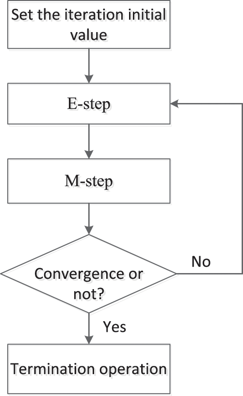
Figure 8: The solving process of GMM based on the EM algorithm

(1) E-step

First, estimate the probability that each component generates the data. Here, we mark the probability of data xi generated by the mth component as γ(i,m), as shown in formula (24).

γ(i,m)=πmN(xi|μm,Σm)∑j=1MπjN(xi|μj,Σj).(24)

(2) M-step

Next, iteratively solve the parameter values according to the calculation results of the previous step.

μm=1Nm∑i=1Nγ(i,m)xi,(25)

Σm=1Nm∑i=1Nγ(i,m)(xi−μm)(xi−μm)T,(26)

πm=NmN,(27)

where Nm=∑i=1Nγ(i,m), repeat the above E-M steps until the value of the log-likelihood function (formula (23)) no longer changes significantly.

lnp(x|π,μ,Σ)=∑i=1Nln{∑m=1MπmN(xi|μm,Σm)}.(28)

3.4.3 HMM

As we all know, the hidden Markov model (HMM) is a classic machine learning model which has proved its value in language recognition, natural language processing, pattern recognition, and other fields [68,69]. This model describes the process of generating a random sequence of unobservable states from a hidden Markov chain and then generating the observed random sequence from each state. Among them, the transition between the states and the observation sequence and the state sequence have a certain probability relationship [70]. The hidden Markov model is mainly used to model the above process.

We assume that M and N represent the set of all possible hidden states and the set of all possible observed states, respectively. Then M and N are expressed as follows:

M={m1,m2,…,mP},N={n1,n2,…,nQ},(29)

where P and Q are the number of possible hidden states and the number of possible observed states, respectively, which are not necessarily equal.

In a sequence of length T, U and V correspond to the state and observation sequences, respectively, as follows:

U={u1,u2,…,uT},V={v1,v2,…,vT},(30)

where the subscript of each element represents the moment. That is, the state sequence and the observation sequence elements are successively related. Any hidden state ut∈M and any observed state vt∈N. Therefore, the graph model structure of the above hidden Markov model is shown in the following Fig. 9.

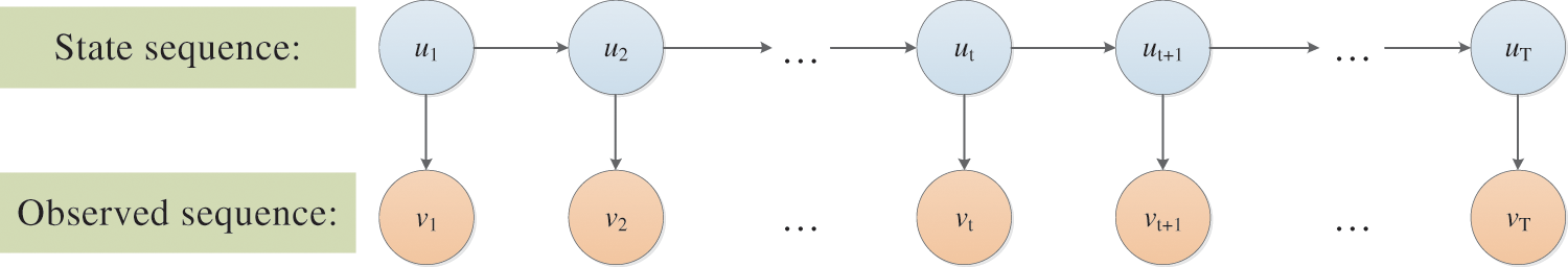
Figure 9: Graph model structure of hidden Markov model

To facilitate the solution, assume that the hidden state at any moment is only related to its previous hidden state. The hidden state at time t is ut=mi and the hidden state at time t+1 is ut+1=mj, then the transition probability of HMM state aij from time t to time t+1 can be obtained as follows:

aij=P(ut+1=mj|ut=mi).(31)

Thus, the state transition matrix A can be obtained:

A=[aij]P×P.(32)

Assuming that the observed state at any moment is only related to the hidden state at the current moment when the hidden state at time t is ut=mj and the corresponding observed state is vt=nk, then the probability bj(k) generated by the observed state nk at this time satisfies the following equation under the hidden state mj.

bj(k)=P(vt=nk|ut=mj).(33)

In this way, bj(k) can form the probability matrix B generated by the observed state.

B=[bj(k)]P×Q.(34)

In addition, we define the probability distribution Π of hidden states at time t=1 as follows:

Π=[π(i)]P,(35)

where π(i)=P(u1=mi), Π is an n-dimensional vector with each element representing the probability of being in a certain state at time t=1. In this way, the initial probability distribution of hidden states Π, the state transition probability matrix A, and the observed state probability matrix B can determine the HMM model, which can be expressed as follows [71]:

λ=(A,B,Π).(36)

Here, Π and A determines the sequence of states, and B determines the sequence of observations.

3.4.4 Other Classification Approaches

In addition to the above classification algorithms (SVM [72–75,43,61], GMM [76,77], HMM [70,69,78]), some other classification algorithms are used for posture recognition, such as k-nearest neighbor (k-NN) [79], random forest (RF) [80–82], Bayesian classification algorithm [83], decision tree (DT) [72,84,85], linear discriminant analysis [86,60], naïve Bayes (NB) [72,87], etc.

4  Deep Neural Network‑Based Approach

Deep learning mainly uses neural network models, such as convolutional neural network (CNN), deep neural network (DNN), recurrent neural network (RNN), transfer learning, attention model, and long short-term memory (LSTM), as parameter structures to optimize machine learning algorithms.

This method is an end-to-end learning method, which does not require manual operation, but relies on the algorithm to automatically extract features, starting directly from the original input data, and automatically completes feature extraction and model learning through a hierarchical network [17]. In recent years, it has been widely used in many fields and achieved remarkable results, such as image recognition, intelligent monitoring, text recognition, semantic analysis, and other fields. Human posture recognition based on deep learning can quickly fit the human posture information in the sample label so as to generate a model with posture analysis ability.

4.1 Posture Estimation

Regarding network architecture, deep learning-based posture estimation is divided into a single-stage approach and a multi-stage approach. The usual difficulty of single-stage networks lies in the subsequent feature fusion work, and multi-stage networks generally repeat and superimpose a small network structure.

Since the number and position of people in the image are unknown in advance, multi-body posture estimation is more difficult than single-body posture estimation, which is usually divided into two ideas: top-down and bottom-up. The former is first to incorporate person detectors, then estimate each part, and finally calculate the pose of each person. The latter is to detect all parts in the image, the parts of each person, and then use a certain algorithm to associate/group the parts belonging to different people. The algorithms mainly include CPM [88], stacked hourglass networks [89], and MSPN [90]. Single-stage approaches are all Top-down, such as CPN [91] and simple baselines [92].

4.2 Convolutional Neural Networks

In posture recognition, convolutional neural networks (CNN) have achieved good results. In the system designed by Yan et al. [93], CNN is used to learn and predict the preset driving posture automatically. Wang [94] used CNN to design a human posture recognition model for sports training. CNN has also been successfully used for capture posture detection [95]. Rani et al. [96] adopted the lightweight network of convolution neural network-long short-term memory (CNN-LSTM) for classical dance pose estimation and classification. Zhu et al. [97] proposed a two-flow RGB-D faster R-CNN algorithm to achieve automatic posture recognition of sows, which applied the feature level fusion strategy.

The neurons in each layer of convolutional neural networks are arranged in three dimensions (width, height, and depth). It should be noted that depth here refers to the number of layers of the network. The convolutional neural network is mainly composed of the input layer, convolutional layer (CL), ReLU layer, pooling layer (PL), and fully connected layer (FCL). A simple diagram of CNN is shown in Fig. 10.

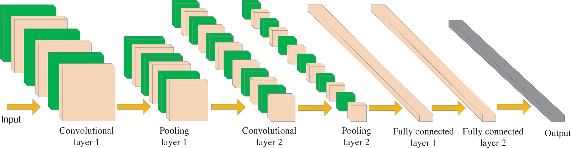
Figure 10: A simple diagram of CNN

The core layer of the convolutional neural network is the convolutional layer, which is composed of several convolution units. The important purposes of dimension reduction and feature extraction are achieved through convolution operation. In the first layer of the convolution layer, only some low-level features, such as edges, lines, and angles, can be extracted. In contrast, more complex posture features need to be extracted from more layers of iteration.

The pooling layer is sandwiched between continuous convolution layers to compress the amount of data and parameters, improve identification efficiency and effectively control overfitting. A pooling layer is actually a nonlinear form of drop sampling.

Generally, the full connection layer is in the last few layers and is used to make the final identification judgment. Their activation can be matrix multiplication, and then the deviation is added.

4.3 Improved Convolutional Neural Networks

Since the sparse network structure of the traditional CNN cannot retain the high efficiency of dense computation of a fully connected network, and the classification results are inaccurate, or the convergence speed is slow due to the low utilization of convolutional features in the experimental process, so many researchers have carried out various optimization of the CNN algorithm.

For example, by using batch normalization (BN), the distribution of input values of any neuron in each layer of the neural network is forced to return to the normal distribution with a mean of 0 and a variance of 1 (or other), so that the activated input values fall in the sensitive area of the input, thus avoiding the vanishing gradient [98].

Deep residual networks address network degradation using residual learning with identity connections [99]. CNN-LSTM provides solutions to complex problems with large amounts of data [96]. Since target tracking methods based on traditional CNN and correlation filters are usually limited to feature extraction with scale invariance, multi-scale spatio-temporal residual network (MSST-ResNet) can be used to realize multi-scale feature and spatio-temporal interaction between the flows of spatial and time [100], which is also regarded as an extension of residual network architecture. Bounding box regression and labeling from raw images via faster R-CNN showed high reliability [101]. In human posture recognition, many networks based on CNN have emerged (such as stacked hourglass networks, MSPN, CPM, and HRNet [102]).

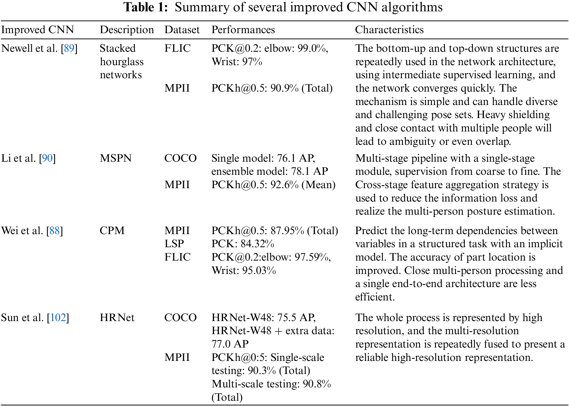
Stacked hourglass networks show good performance in human posture estimation based on successive pooling and upsampling steps to capture and integrate information at all image scales. The network is combined with intermediate supervision for bottom-up, top-down repetitive processing [89]. The stacked hourglass model is formed by concatenating hourglass modules, each consisting of many residual units, pooling layers, and upsampling layers [103], so it is able to capture all information at each scale and combine these features to output pixel-level predictions.

In the study by Alejandro Newell et al. [89] using a single pipeline with skip layers to preserve spatial information at each resolution, the topology of the hourglass is symmetric. That is, for each layer that exists downward, there is an upper-level corresponding to it. After reaching the output resolution of the network, the final network prediction is completed by two successive rounds of 1×1 convolution.

The output of the network is a set of heat maps, and for a given heat map, the probability of a joint occurring at each pixel will be predicted. The remaining modules are used as much as possible in the stacked hourglass network, and local and global features are integrated by each hourglass module, which is further understood in subsequent bottom-up and top-down processing phases. The hourglass modules do not share the weight with each other. The filters are all less than or equal to 3 × 3, and the bottleneck limits the total number of parameters per layer, thus reducing the overall memory usage [89].

Li et al. [90] first introduced the multi-stage pose estimation network (MSPN), which adopted ResNet-based global net as a single-stage module and used a cross-stage feature aggregation strategy, that is, two independent information streams are introduced from the downsampling unit and upsampling unit of the previous stage to the downsampling process of the current stage for each scale, and 1×1 convolution is added to each stream for feature aggregation to alleviate the problem of information loss during repeated upsampling and downsampling of multi-stage networks.

Furthermore, feature aggregation can be regarded as an extended residual design that helps solve the vanishing gradient. The multi-stage pose estimation network is designed as a multi-branch supervision method from coarse to fine. Different Gaussian kernel sizes are used at different stages, and the closer the stage kernel-size is to the input, the larger the stage kernel-size will be. Multi-scale supervision is introduced to perform intermediate supervision with four different scales at each stage, resulting in a large amount of contextual information at different levels to help localize challenging poses.

Wei et al. [88] introduced the first pose estimation model based on deep learning, which is called the convolutional pose machine (CPM). CPM combines the advantages of a deep convolutional architecture with a pose machine framework consisting of a series of convolutional networks. In other words, the pose machine’s prediction and image feature calculation modules are replaced by deep convolutional architecture, which allows the image and context features to be directly learned from the data to represent these networks. The convolutional architecture is fully differentiable, and all stages of the CPM can be trained end-to-end. In this way, the problem of structured prediction in computer vision can be solved without inferring the graphical model. Furthermore, the method of intermediate supervision is also used to solve the gradient disappearance problem in the cascade model training process.

The high-resolution network (HRNet) was proposed by Sun et al. [102], showing superior performance in human body pose estimation. This network will connect sub-networks from high resolution to low resolution in parallel to maintain high-resolution expression. Furthermore, the predicted heatmaps are more accurate by performing repeated multi-scale fusions to obtain high-resolution features with low-resolution representations of the same depth and similar levels.

We have introduced several typical CNN-based posture recognition algorithms above, which all have their own characteristics, and the summary is shown in Table 1.

4.4 Lightweight Network

The practice proves that a large number of convolutional neural network models have a significant effect on posture recognition. However, with the increasing complexity of convolutional neural network models, the number of layers of the model will gradually deepen accordingly, resulting in an increasing number of parameters, which will require more computing resources. Moreover, with the support of Internet of Things (IoT) technology and smart terminals, such as mobile phones and embedded devices, there is an increasing demand for porting human posture recognition networks to resource-constrained platforms [104]. Therefore, lightweight research on the convolutional neural network model is gradually carried out. The emerging lightweight network models mainly include Squeeze Net [105], Mobile Net [106], Shuffle Net [107], Xception [108], and Shuffle Net V2 [109].

4.4.1 Spatial Separable Convolutions

Spatially separable convolution (SSC) mainly refers to splitting or transforming the convolution kernel, then performing convolution calculations separately, which mainly deals with the two spatial dimensions of image width and height and the convolution kernel. A spatially separable convolution splits a kernel into two smaller kernels.

For example, before a 3×3 convolution core is split, nine times multiplication is required to complete a convolution. After being split into a 3×1 and 1×3 convolution core, three times multiplication is required for each convolution, and a total of 6 multiplications for the combination of the two convolutions can achieve the same effect as before [110], as shown in Fig. 11. The cost of multiplication is reduced, so the computational complexity is reduced, and the network can run faster. It should be noted that not all convolution kernels can be split into two smaller ones.

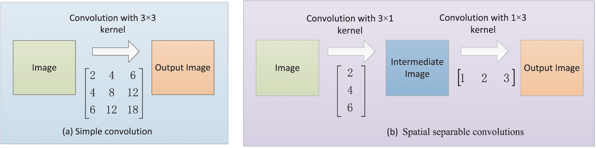
Figure 11: An example of spatial separable convolutions

4.4.2 Depthwise Separable Convolution

In depthwise separable convolution (DSC), one convolution kernel can also be split into two small convolution kernels, but different from spatially separable convolution, depthwise separable convolution can be applied to those convolution kernels that cannot be split, and then perform two calculations for these two convolution kernels: depthwise convolution and pointwise convolution, which greatly reduces the amount of computation in the convolution process.

Depthwise convolution is a channel-to-channel convolution operation that establishes a k×k convolution kernel for each channel of input data. A convolution kernel convolves a channel, and a channel is convolved only by a convolution kernel. In this process, the number of generated feature mapping channels is exactly equal to the number of input channels [111].

Pointwise convolution operations are very similar to regular convolution operations. A 1×1 convolution kernel is implemented on every channel completed by depthwise convolution. The size of the pointwise convolution kernel is 1×1×L, where L is the number of channels on the upper layer. The mapping in the previous step is weighted in the depth direction by the convolution operation to generate a new feature map pointwise convolution.

The spatial dimension can be processed by depthwise separable convolution, and the matrix can also be divided by the depth of the convolution kernel. It is to segment the channels of the convolution kernel instead of directly decomposing the matrix.

4.4.3 Feature Pyramid Networks

The feature pyramid network (FPN) is designed according to the concept of a feature pyramid. Instead of the feature extractor of detection models (such as faster R-CNN), FPN generates multi-layer feature maps and pays attention to both the texture features of the shallow network and semantic features of the deep network when extracting features.

FPN includes three parts: bottom-up path, top-down path, and lateral connection [112], as shown in Fig. 12. The bottom-up path calculation is a feature hierarchy composed of feature maps of multiple scales, which is the traditional convolutional network to achieve feature extraction. With the deepening of the convolution network, the spatial resolution decreases, and the spatial information is lost, but the semantic value of the network layer increases correspondingly and is more detected.

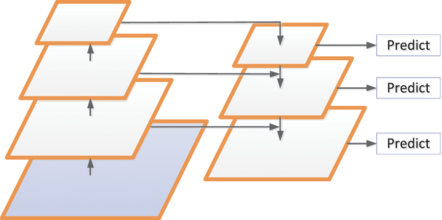
Figure 12: Schematic diagram of FPN network structure

The top-down path builds higher-resolution layers based on semantically richer layers. These features are then augmented by horizontal connections using the features in the bottom-up path [112]. The feature maps of the same spatial size of the bottom-up path and the top-down path are merged by each horizontal connection.

4.5 Batch Normalization

For a neural network, the parameters will be continuously updated with the gradient descent, which will cause changes in the data distribution of internal nodes, that is, the internal covariance translation phenomenon. In this case, the above problems can be solved by batch normalization (BN), and the speed of model training and the performance of network generalization can be significantly improved [113].

The main idea of BN is that any layer in the network can be normalized, and the normalized feature graph can be re-scaled and shifted to make the data meet or approximate the Gaussian form of distribution. Batch normalization can reparameterize almost any deep network, addressing the situation where the data distribution in the middle layers changes during training [114]. Like the convolution layer, activation function layer, pooling layer, and fully connected layer, batch normalization is also a network layer. The forward transmission process of the BN network layer is shown in Eqs. (37)–(40) and Fig. 13.

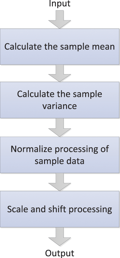
Figure 13: The forward transmission process of the BN network layer

μg=1n∑i=1nxi,(37)

σg=21n∑i=1n(xi−μg)2,(38)

xiΔ=xi−μgσg2+τ,(39)

BNα,β(xi)=αxiΔ+β.(40)

Here, μg refers to mini-batch mean, σg2 refers to mini-batch variance, n refers to the mini-batch size, and xiΔ denotes the normalization process. We define τ as a very small value to prevent the denominator from being zero. To maintain the expressiveness of the model, we introduce two learning parameters α and β, α refers to the scale factor, and β refers to the shift factor.

In convolutional neural networks, batch normalization occurs after the convolution computation and before the activation function is applied. If the convolution calculation outputs multiple channels, the outputs of these channels should be batch normalized separately, and each channel has the independent scale and shift parameters, which are all scalars.

4.6 Deep Residual Network

In conventional neural networks, the continuous increase of network depth will lead to the gradual increase of accuracy until saturation and then rapid decline, resulting in the difficulty of deep network training, that is, network degradation, which may be caused by the model being too large and the convergence speed too slow. The degradation problem can be solved by the deep residual network (DRN) [115]. The network layer can be made very deep through this residual network structure, and the final classification effect is also very good.

In the residual network structure, for a neural network with a stacked-layer structure, assuming the input is x, H(x) denotes the learned feature, and the residual that can be learned is expected to be denoted as F(x)=H(x)−x, so the original learned feature obtained as F(x)+x. H(x) can be implemented by a feedforward neural network with “shortcut connections” [115], as shown in Fig. 14. When the residual F(x) is equal to 0, only the identity mapping is completed by the stacking layer, and the goal of the later learning is to approximate the residual result to 0 so that with the deepening of the network, the network performance will not be degraded.

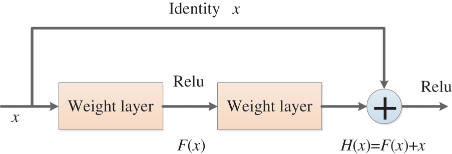
Figure 14: The basic residual block

4.7 Dropout Technology

In the deep neural network model, if the number of neural network layers is too large, the training samples are few, or the training time is too long, it will lead to the phenomenon of overfitting [116]. Dropout technology can be used to reduce overfitting to prevent complex co-adaptation to training data [117].

In the neural network using dropout technology, a batch of units is randomly selected and temporarily removed from the network at each iteration in the training stage, keeping these units out of forward inference and backward propagation [116].

It should be noted that instead of simply discarding the outputs of some neural units, we need to change the values of the remaining outputs to ensure that the expectations of the outputs before and after discarding remain unchanged. In general, a fixed probability p that each cell retains can be selected using the validation set, and the probability p is often set to 0.5. Still, the optimal retention probability is usually closer to 1 for input cells. In networks with dropout, the generalization errors of various classification problems can be significantly reduced using the approximate averaging method.

Suppose we want to train such a neural network, as shown in Fig. 15a. After Dropout is applied to the neural network, the training process is mainly the following:

  (i)   Randomly delete half of the hidden neurons in the network. Note that these deleted neurons are only temporarily deleted, not permanently deleted, and the input and output neurons remain unchanged, as shown in Fig. 15b.

 (ii)   The input is then propagated forward along the modified network, and the loss result is propagated back along the modified network. After this procedure was performed on a small group of training samples, the parameters of the neurons that were not deleted were updated according to the random gradient descent (SGD) method.

(iii)   Restore the deleted neuron. At this time, the deleted neuron parameters keep the results before deletion, while the non-deleted neuron parameters have been updated. The above process is repeated continuously.

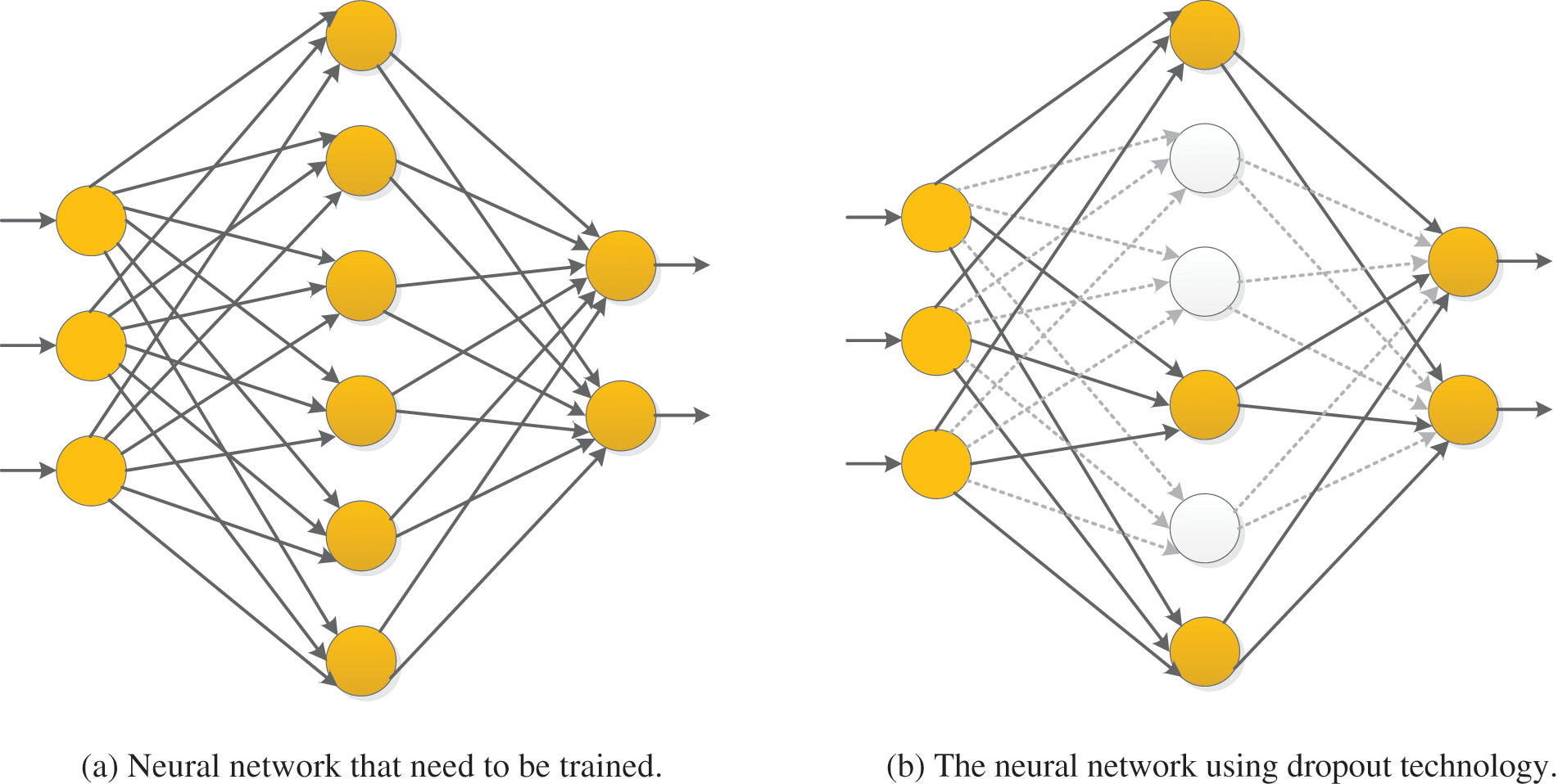
Figure 15: A neural network using dropout technology

4.8 Advanced Activation Functions

In a neural network, an important purpose of using multi-layer convolution is to use the size of different convolution kernels to extract image features at different convolution kernel scales. The convolution algorithm is composed of a mass of multiplications and additions, so the convolution algorithm is also linear and can be considered a linear weighting operation through the convolution kernel. The convolutional neural network composed of many convolution algorithms will degenerate into a simple linear model without introducing nonlinear factors, making the multi-layer convolution meaningless.

Therefore, adding a nonlinear function after the convolution of each layer of the neural network can complete the linear isolation of the two convolution layers and ensure that each convolution layer completes its own convolution task. Currently, the common activation functions mainly include sigmoid, tanh, rectified linear unit (ReLU), etc. Compared with the traditional activation functions of neural networks, such as sigmoid and tanh, RELU has the following advantages: (i) When the input of the ReLU function is positive, the gradient saturation will not occur in the network. (ii) Since the ReLU function has only a linear relationship, its calculation speed is faster than sigmoid and tanh. The definition of the ReLU function is shown in Eq. (41) [118]:

hReLU(xi)=max(0,xi),(41)

where xi is the input in the ith channel. There are many variants of the ReLU function, such as parametric ReLU, leaky ReLU, random ReLU, etc. Each activation function has advantages in one or several specific deep learning networks.

Leaky ReLU (LReLU) is similar to ReLU, except that the input is less than 0. In the ReLU function, all negative values are zero, and the outputs are non-negative. In contrast, in the Leaky ReLU, all negative values are assigned a non-zero slope with a negative value and a small gradient [119]. The Leaky ReLU activation function can avoid zero gradients, which is defined as follows:

hLReLU(xi)={xi,if xi>0aixi,if xi≤0.(42)

Here, ai is a fixed parameter, usually with a value of 0.01. In the process of backpropagation, the gradient can also be calculated for the part of the Leaky ReLU activation function input less than zero, which can avoid the problem of gradient direction aliasing.

Parametric ReLU (PReLU) adaptively learns to rectify the parameters of linear units and is able to improve classification accuracy at a negligible extra computational cost [120]. The definition of the PReLU function is shown in Eq. (43):

hPReLU(xi)={xi,if xi>0βixi,if xi≤0.(43)

Here, βi is responsible for controlling the slope of the negative semi-axis, and the activation functions of different channels can be different. When the value of βi is 0, PReLU can be regarded as ReLU. If the value of βi is small and fixed, then PReLU can be considered Leaky ReLU.

Randomized ReLU (RReLU) can be understood as a variant of Leaky ReLU. The definition of RReLU function is shown as follows:

hRReLU(xji)={xji,if xji>0ajixji,if xji≤0.(44)

Here, xji represents the input of the ith channel in the jth example, aji is a random value drawn from a uniform distribution U(l,u).

aji∼U(l,u),l<u and l, u∈[0,1).(45)

The diagrams of ReLU, LReLU, PReLU, and RReLU are shown in the following Fig. 16 [121].

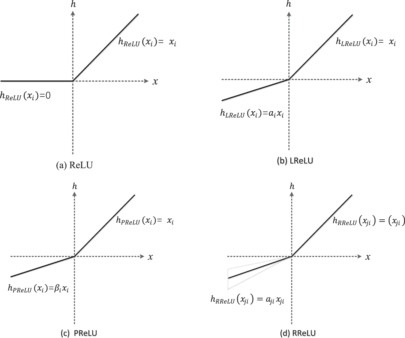
Figure 16: The diagrams of ReLU, LReLU, PReLU, and RReLU

5  Advanced Neural Networks

In order to improve the performance of the system, some advanced neural networks are studied in the field of posture recognition, such as transfer learning, ensemble learning, graph neural networks, explainable deep neural networks, etc.

5.1 Transfer Learning

Transfer learning (TL) refers to the transfer of the trained model parameters to the new model to help the new model training [122]. Transfer learning technology has been used in posture recognition. Hu et al. [123] used transfer learning in their sleep posture system, and the system accuracy and real-time processing speed were much higher than the standard training-test method. Ogundokun et al. [124] applied the transfer learning algorithm with hyperparameter optimization (HPO) to human posture detection. The experiments show that the algorithm is superior to the algorithm using image enhancement in terms of training loss and verification accuracy, but the system’s complexity increased after the algorithm was used. Long et al. [125] developed a yoga self-training system using transfer learning techniques.

Considering that most data or tasks are related, through transfer learning, we can share the learned model parameters with the new model in some way to speed up and optimize the learning efficiency of the model. It is one of the advantages of transfer learning that we do not need to learn from zero like most networks. In addition, in the case of small data sets, transfer learning can get good results, and we can also use transfer learning to reduce training cost sets.

5.2 Ensemble Learning

Ensemble learning (EL) is to construct and combine multiple machine learning machines to complete learning tasks. The process generates a group of “individual learning machines” and then combines them with a certain strategy [126]. Individual learning machines are common machine learning algorithms, such as decision trees and neural networks [127]. Ensemble learning can be used for classification problem integration, regression problem integration, feature selection integration, outlier detection integration, and so on.

Ensemble learning is used in sensor-based posture recognition systems to overcome the problems of data imbalance, instant recognition, sensor deployment, and selection when collecting data with wearable devices [128]. Liang et al. [129] designed a sitting posture recognition system using an ensemble learning classification model to ensure the generalization ability of the system. Esmaeili et al. [130] designed a posture recognition integrated model by superimposing two classification layers based on the deep convolution method.

5.3 Graph Neural Networks

Graph neural networks (GNN) is a framework that uses deep learning to learn the graph structure data directly. Aggregating features of adjacent nodes calculate the features of each node, and the graph dependency is established by passing messages between nodes [131]. In GNN, graph properties (such as points, edges, and global information) are transformed without changing the connectivity of the graph.

GNN has achieved excellent results in posture recognition tasks. Guo [132] formed a multi-person posture estimation algorithm based on a graph neural network by using multilevel feature maps, which greatly improved the positioning accuracy of each part of the human body. Li et al. [133] used the graph neural network to optimize posture graphs, which achieves good efficiency and robustness. Taiana et al. [134] constructed a system based on graph neural networks that can produce accurate relative poses.

In recent years, the variants of GNN variants, such as graph convolutional networks (GCNs), graph attention networks (GATs), and gated graph neural networks (GGNNs), have shown breakthrough performance in many posture recognition tasks [135–137].

6  Analysis and Discussion

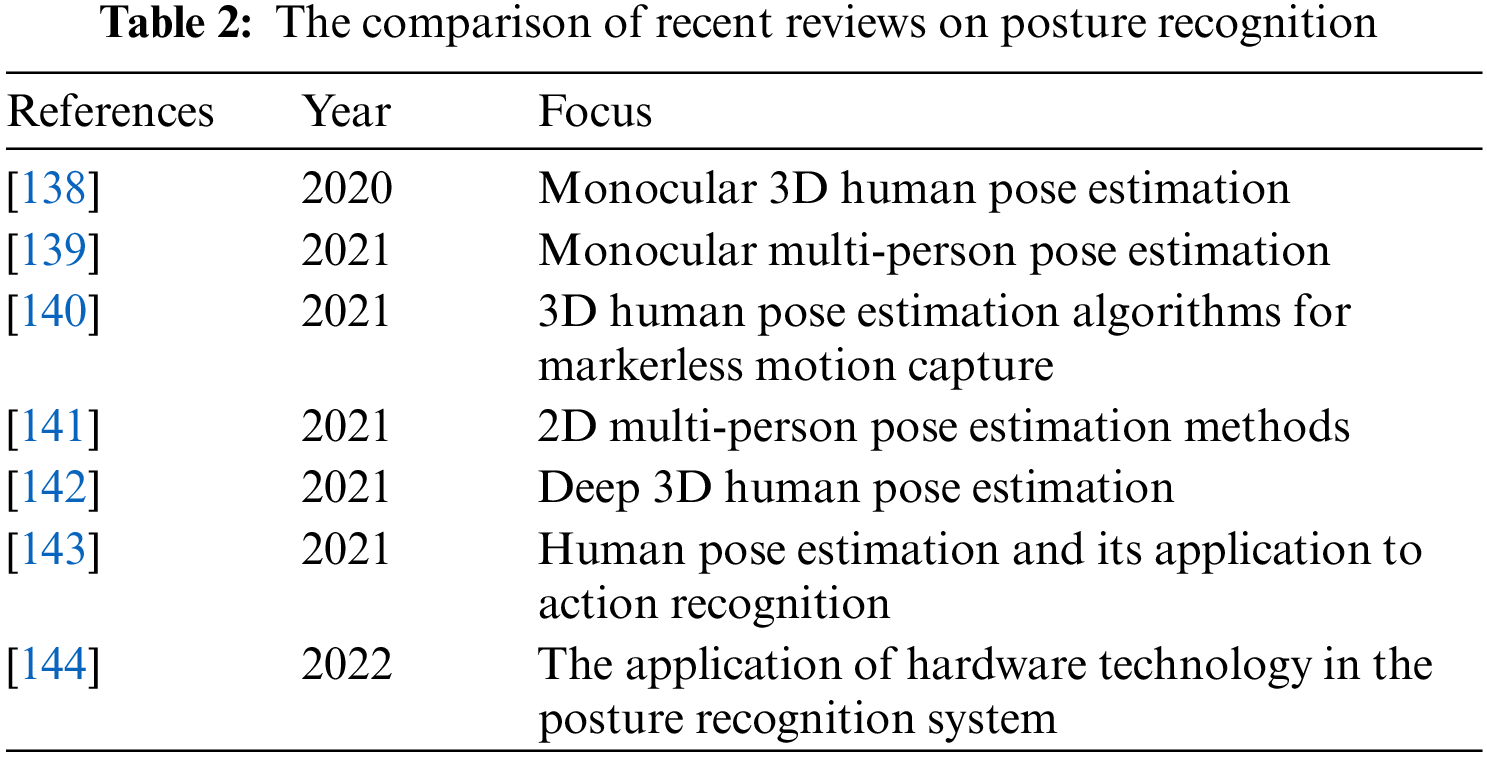
We have detailedly reviewed the techniques and methods of posture recognition, including the process of posture recognition, feature extraction, and classification techniques. Compared with the existing reviews in recent years, this paper presents the following advantages: (i) This paper combs the pose recognition technologies and methods based on traditional machine learning and deep learning-based posture recognition technologies and methods and summarizes and analyzes 2D and 3D datasets, which is more comprehensive in content; (ii) In order to timely share the latest technologies and methods of posture recognition with readers, this review focuses on the latest development of posture recognition technologies and methods. The literature on posture recognition technologies and methods is relatively new, and most of them are related research papers from the past five years, which have been updated in time. We list the comparison of recent reviews on posture recognition as shown in Table 2.

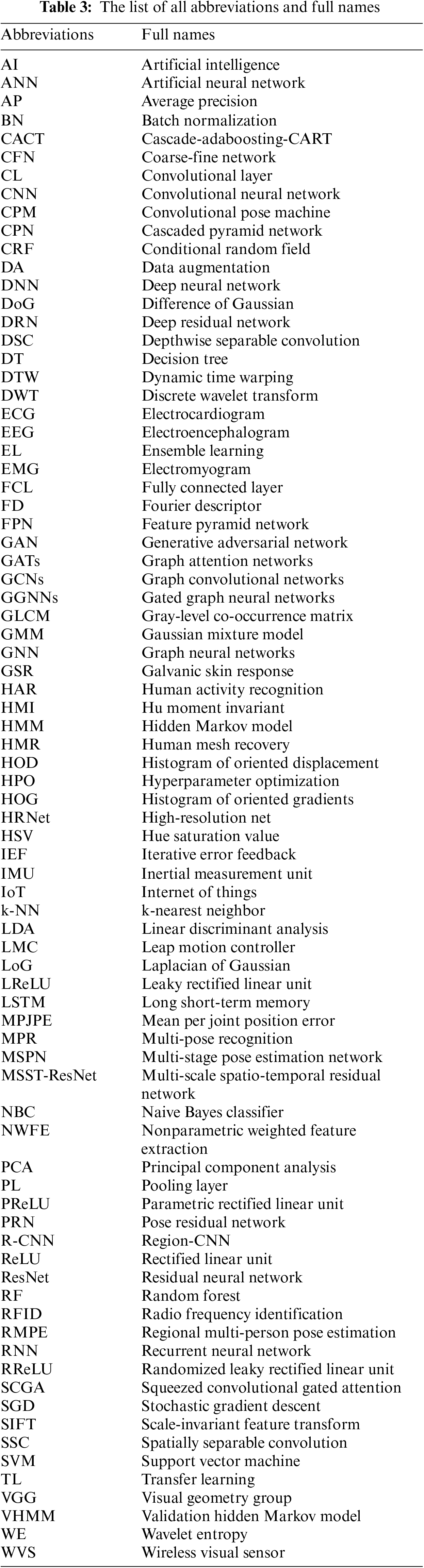
To help understand more clearly, we created a table of abbreviations and corresponding full names for posture recognition terms as follows (Table 3):

6.1 Main Recognition Techniques

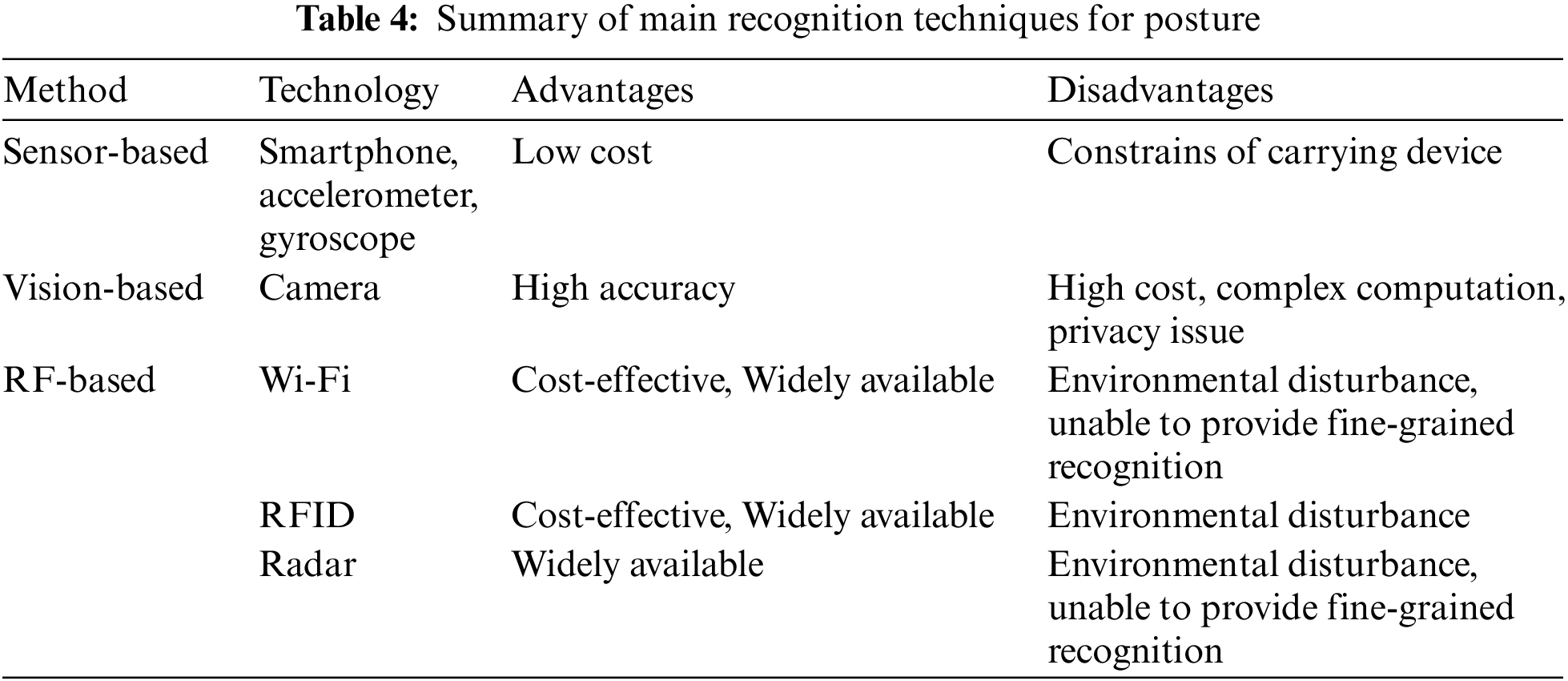
According to data acquisition, posture recognition technology is divided into sensor-based recognition technology, vision-based recognition technology, and RF-based recognition technology.

Sensor-based recognition methods are less costly and simple to operate but are limited to devices and require the real-time wearing of sensors [17,145].

Vision-based recognition method has high accuracy and overcomes the problem of wearing. It is easy to obtain the trajectory, contour, and other information about human movement. However, this method is affected by light, background environment, and other factors and is prone to recognition errors due to occlusion and privacy exposure [146,147].

RF-based identification technology has the characteristics of non-contact and is very sensitive to environmental changes. It is easily affected by the human body’s absorption, reflection, and scattering of RF signals [31]. The characteristics of the three recognition methods are shown in Table 4.

6.2 2D Posture Recognition and 3D Posture Recognition

According to the difference in human posture dimensions, the human posture recognition task can be divided into two-dimensional human posture recognition and three-dimensional human posture recognition. The purpose of two-dimensional human posture recognition is to locate and identify the keypoints of the human body. Then these key points are connected in the order of joints, which are projected on the two-dimensional plane of the image to form the human skeleton.

There are currently many 2D recognition algorithms, and the accuracy and processing speed have been greatly improved. However, the keypoints of 2D are greatly affected by wearing, posture and perspective. They are also affected by the environment, such as occlusion, illumination, and fog, which require high requirements for data annotation. In addition, the keypoints of 2D are not easy to estimate the positions between human body parts through vision.

3D posture recognition can give images a more stable and understandable interpretation. In recognition of human 3D posture, the 3D coordinate position and angle of human joints are mainly predicted. We can use the 3D posture estimator to convert objects in the image into 3D objects by adding depth to the prediction, that is, to realize the mapping between 2D keypoints and 3D keypoints. There are two specific methods: One is to directly regress 3D coordinates from 2D images [148,149], and the other is to obtain the data of 2D first and then “lift” to 3D posture [150,151].

In 3D posture recognition, due to the addition of depth information on the basis of 2D posture recognition, the expression of human posture is more accurate than in 2D, but there will be occlusion, and it also faces challenges such as the inherent deep ambiguity and inadequacy in single-view 2D to 3D mapping, and the lack of large outdoor datasets. Currently, the mainstream datasets are established in the laboratory environment, and the model’s generalization ability is weak. In addition, there is a lack of special posture datasets, such as falling and rolling.

6.3 Recognition Based on Traditional Machine Learning and Deep Neural Network

Traditional machine learning-based recognition methods mainly describe and infer human posture based on the human body models and extract image posture features through algorithms, which have high requirements on feature representation and spatial position relationship of keypoints. Excluding low level features (such as boundary and color), typical high-level features, such as scale-invariant feature transformation and gradient histogram, have stronger expression ability and can effectively compress the spatial dimension of features, showing advantages in terms of time efficiency.

Posture recognition based on deep learning can be trained and learned through the image data of the network model, and the most effective representation method can be directly obtained. The core of posture recognition based on deep learning is the depth of neural networks. Semantic information is extracted from the image through a convolutional neural network, richer and more accurate and reflects better robustness than artificial features.

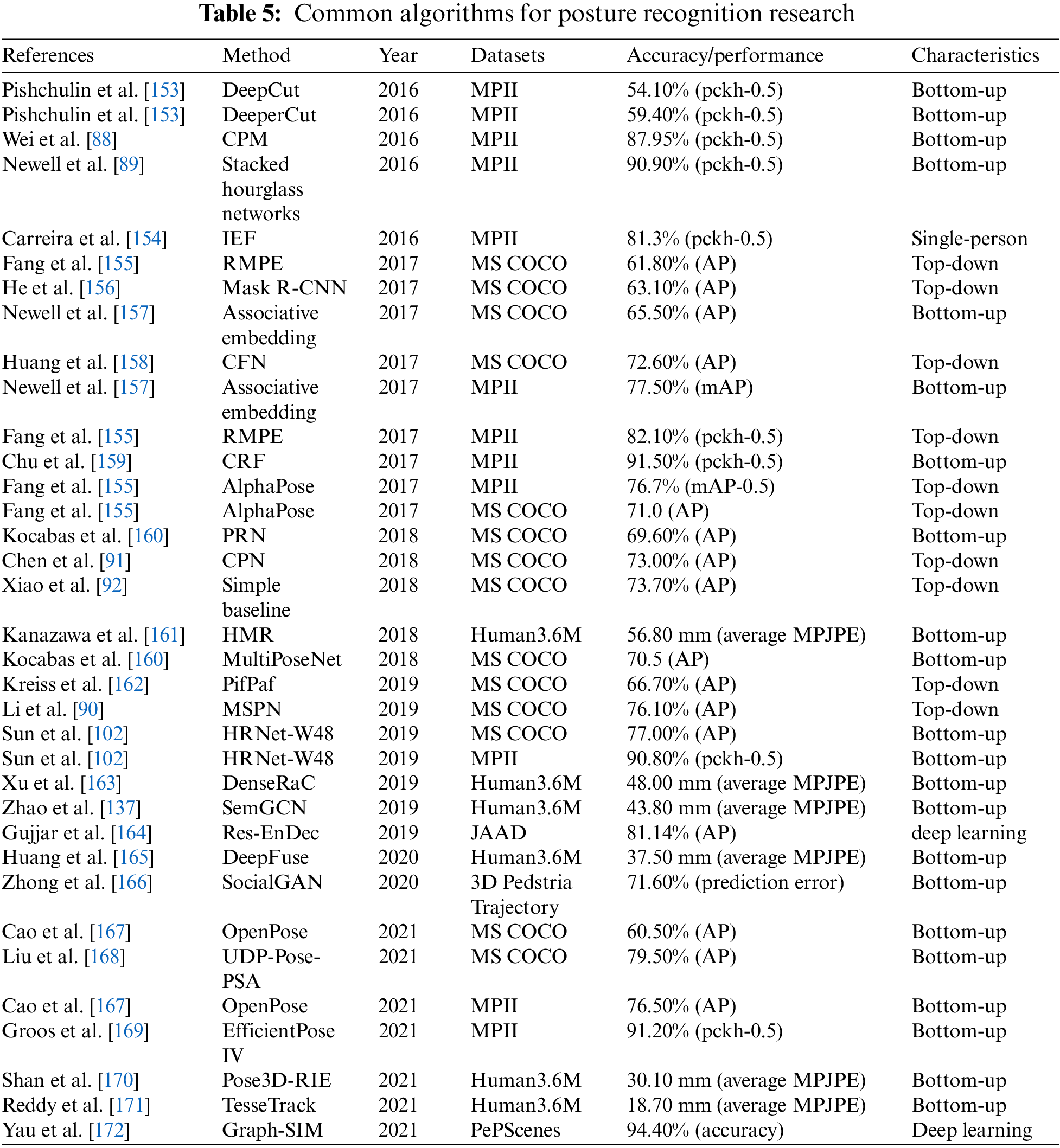
Moreover, the expressive ability of the network model will increase exponentially with the increase of the network stack number. However, overcoming factors such as occlusion, inadequate training data, and depth blur is still difficult. The commonly used posture recognition algorithms [143,152] in recent years are shown in Table 5.

6.4 Datasets

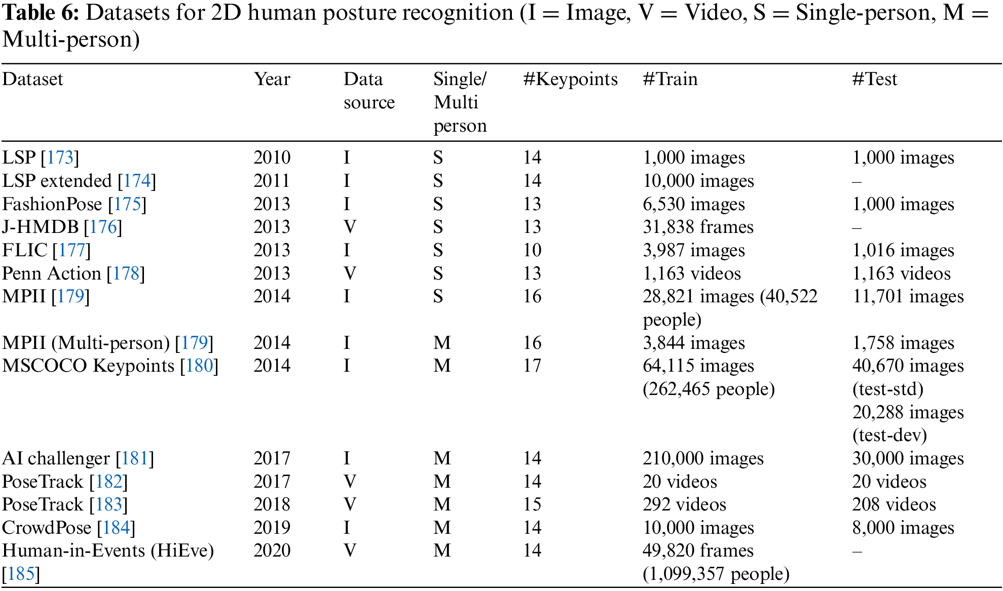
In the field of posture recognition, the successful application of deep learning has significantly improved the accuracy and generalization ability of two-dimensional posture recognition, where the datasets play a crucial role in the system [143]. We list widely used 2D posture benchmark datasets, as shown in Table 6.

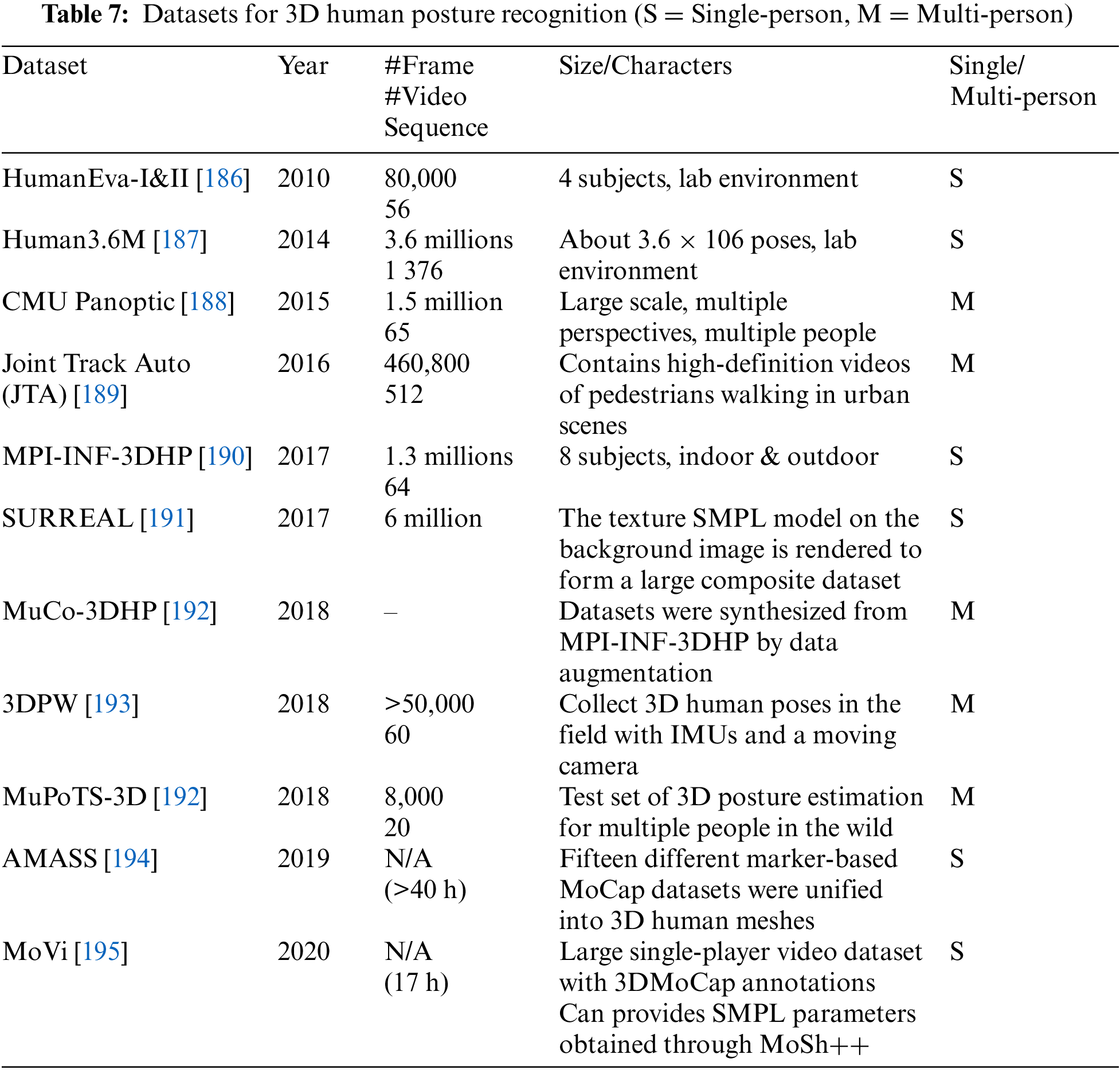
Compared with 2D posture recognition, 3D posture recognition faces more challenges, among which deep learning algorithms rely on huge training data. However, due to the difficulty and high cost of 3D posture labeling, the current mainstream datasets are collected in the laboratory environment and lack large outdoor datasets. This will inevitably affect the generalization performance of the algorithm on outdoor data [138,143]. The widely used 3D posture recognition datasets are shown in Table 7.

6.5 Current Research Direction

At present, posture recognition is divided into the following research directions:

(1)   Pose machines. The pose machine is a mature 2D human posture recognition method. In order to make use of the excellent image feature extraction ability of the convolutional neural network, the convolutional neural network is integrated into the framework of the pose machine [88].

(2)   Convolutional network structure. In recent years, significant progress has been made in posture recognition based on convolutional network structure, but there is still room for optimization in recognition performance. Many researchers focused on the optimization of convolutional network structures, and some optimization models were proposed, such as stacked hourglass network [89], iterative error feedback (IEF) [154], Mask R-CNN [156], and the EfficientPose [169].

(3)   Multi-person posture recognition in natural scenes. Due to many factors, such as complex background, occlusive congestion, and posture difference in the natural environment, many posture recognition methods with a fine performance in the experimental environment are ineffective in multi-person posture recognition tasks. However, with the development of the field of posture recognition, multi-person recognition in natural scenes is very worthy of study. Fortunately, the recognition of multiple people in natural scenes has attracted the attention of many scholars [155].

(4)   Attention mechanism. By designing different attention mechanism characteristics for each part of the human body, more accurate human posture recognition results can be obtained. Some attention-related strategies have been proposed, for example, the attention regularization loss based on local feature identity to constrain attention weight [135], the convolutional neural network with multi-context attention mechanism is incorporated into the end-to-end framework of posture recognition [159], and the polarization self-attention block is realized through polarization filtering and enhancement techniques [168].

(5)   Data fusion. The performance of the data fusion algorithm directly affects the accuracy of posture recognition and the reliability of the system [196,197]. Data fusion strategies include multi-sensor-based data fusion [17,198,199], position and posture-based fusion [200], multi-feature fusion [201,202], and so on.

7  Conclusion and Future Directions

This paper reviews and summarizes the methods and techniques of posture recognition. It mainly includes the following aspects: (i) The structure and related algorithms based on traditional machine learning and deep neural network are presented; (ii) The background and application of three posture recognition techniques are presented, and their characteristics are compared; (iii) Several common posture recognition network structures based on CNN are presented and compared; (iv) Three typical lightweight network design methods are presented; (v) The commonly used datasets for posture recognition are summarized, and the limitations of 2D and 3D datasets are talked about. In summary, the framework of our review is shown in Fig. 17.

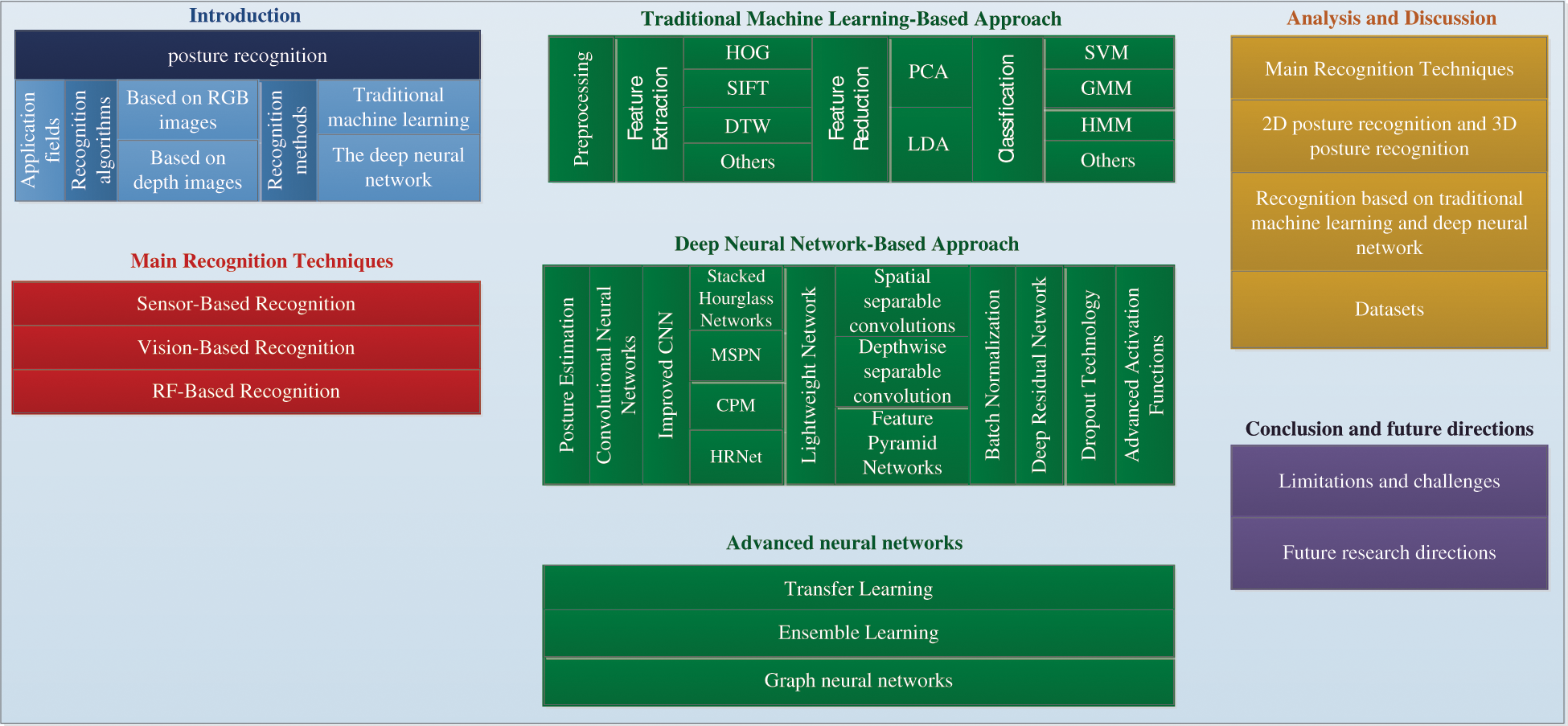
Figure 17: The systematic diagram of our study

7.1 Limitations and Challenges

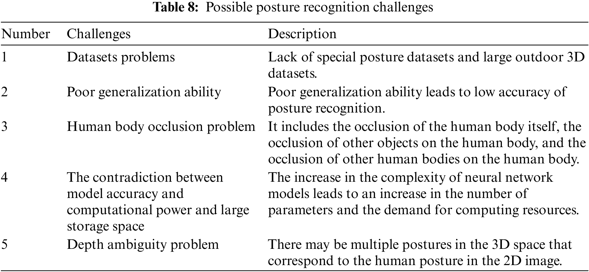
Although the techniques and methods of posture recognition have made great progress in recent years, posture research will still face challenges due to the complexity of the task and the different requirements of different fields. Through the research, we believe that the challenges facing posture recognition at this stage mainly include the following aspects, as shown in Table 8.

(1) Datasets problems

  (i)   Lack of special posture datasets. Currently, the existing public datasets have a large amount of data, but most of the human posture is normal, such as standing, walking, and so on. Lack of special postures, such as falling, crowding, etc.

 (ii)   Lack of large outdoor 3D datasets. The production of 3D posture datasets mostly relies on motion capture equipment, which has restrictions on the environment and the range of human activity, so 3D datasets in outdoor scenes are relatively scarce.

(2) Poor generalization ability

Since many datasets are established in the experimental environment, the generalization ability of the human posture recognition model in natural scenes is poor, and it is difficult to achieve an accurate posture recognition effect in practical applications [203].

(3) Human body occlusion problem

Human body occlusion is one of the most important problems in the process of posture recognition, especially in the natural environment of multi-person posture recognition. Human body occlusion is very common. The phenomenon of human-body occlusion includes the occlusion of the human body itself, the occlusion of other objects on the human body, and the occlusion of other human bodies on the human body [204,205]. The occlusion of the human body has a great influence on the prediction of human body joints.

(4) The contradiction between model accuracy and computational power and large storage space

Deep learning algorithm has become the mainstream method of posture recognition. Many existing posture recognition technologies based on deep learning blindly pursue accuracy, and the design of complex and multi-level networks leads to high requirements on hardware, which is not good for the wide application of neural networks. Therefore, it is particularly important to carry out lightweight design on the network while maintaining recognition accuracy.

(5) Depth ambiguity problem

Depth ambiguity is a problem in 3D posture recognition, which may result in multiple 3D postures corresponding to the same 2D projection. Additional information needs to be added by the algorithm to recover the correct 3D posture [206]. Many approaches attempt to solve this problem by using a variety of prior information, such as geometric prior knowledge, statistical models, and temporal smoothness [207]. However, there are still some unsolved challenges and gaps between research and practical application.

7.2 Future Research Directions

In the future, the research of posture recognition can proceed from the following two aspects of the above discussion of the challenges. (i) Establish an appropriate posture benchmark database, which can be integrated and improved. (ii) The technology based on CNN and other deep neural networks have the potential for improvement, which can be researched in feature extraction, information fusion, and other aspects. (iii) The robustness and stability of body mesh reconstruction under heavy occlusion need to be further explored [208]. (iv) Lightweight network design can be used to solve the contradiction between model accuracy, computing power, and large storage space. It still has a lot of room for improvement in recognition accuracy.

Funding Statement: The paper is partially supported by British Heart Foundation Accelerator Award, UK (AA/18/3/34220); Royal Society International Exchanges Cost Share Award, UK (RP202G0230); Hope Foundation for Cancer Research, UK (RM60G0680); Medical Research Council Confidence in Concept Award, UK (MC_PC_17171); Sino-UK Industrial Fund, UK (RP202G0289); Global Challenges Research Fund (GCRF), UK (P202PF11); LIAS Pioneering Partnerships award, UK (P202ED10); Data Science Enhancement Fund, UK (P202RE237); Fight for Sight, UK (24NN201); Sino-UK Education Fund, UK (OP202006).

Conflicts of Interest: The authors declare that they have no conflicts of interest to report regarding the present study.

References

1. Górriz, J. M., Ramírez, J., Ortíz, A., Martínez-Murcia, F. J., Segovia, F. et al. (2020). Artificial intelligence within the interplay between natural and artificial computation: Advances in data science, trends and applications. Neurocomputing, 410(2), 237–270. https://doi.org/10.1016/j.neucom.2020.05.078 [Google Scholar] [CrossRef]

2. Islam, M. M., Nooruddin, S., Karray, F. (2022). Multimodal human activity recognition for smart healthcare applications. 2022 IEEE International Conference on Systems, Man, and Cybernetics (SMC), pp. 196–203. Prague, Czech Republic, IEEE. [Google Scholar]

3. Lin, C. W., Hong, S., Lin, M., Huang, X., Liu, J. (2022). Bird posture recognition based on target keypoints estimation in dual-task convolutional neural networks. Ecological Indicators, 135, 108506. https://doi.org/10.1016/j.ecolind.2021.108506 [Google Scholar] [CrossRef]

4. Shao, H., Pu, J., Mu, J. (2021). Pig-posture recognition based on computer vision: Dataset and exploration. Animals, 11(5), 1295. https://doi.org/10.3390/ani11051295 [Google Scholar] [PubMed] [CrossRef]

5. Zhang, C., Wang, F., Tian, J. Y. (2018). The recognition of pig posture based on target features and decision tree support vector machine. Science Technology and Engineering, 18, 297–301. [Google Scholar]

6. Chen, C., Zhu, W., Norton, T. (2021). Behaviour recognition of pigs and cattle: Journey from computer vision to deep learning. Computers and Electronics in Agriculture, 187(1–3), 106255. https://doi.org/10.1016/j.compag.2021.106255 [Google Scholar] [CrossRef]

7. Siddiqui, M. (2010). Human pose estimation from a single view point. Computer Vision and Pattern Recognition Workshops (CVPRW2010 IEEE Computer Society Conference, pp. 1–8. San Francisco, CA, USA, IEEE. [Google Scholar]

8. Liu, G., Lin, L., Zhou, W., Zhang, R., Guo, H. (2019). A posture recognition method applied to smart product service. Procedia CIRP, 83(12), 425–428. https://doi.org/10.1016/j.procir.2019.04.145 [Google Scholar] [CrossRef]

9. Jiang, X., Satapathy, S. C., Yang, L., Wang, S. H., Zhang, Y. D. (2020). A survey on artificial intelligence in Chinese sign language recognition. Arabian Journal for Science and Engineering, 45(12), 9859–9894. https://doi.org/10.1007/s13369-020-04758-2 [Google Scholar] [CrossRef]

10. Bao, L., Intille, S. S. (2004). Activity recognition from user-annotated acceleration data. International Conference on Pervasive Computing, pp. 1–17. Linz/Vienna, Austria, Springer. [Google Scholar]

11. Yadav, S. K., Agarwal, A., Kumar, A., Tiwari, K., Pandey, H. M. et al. (2022). YogNet: A two-stream network for realtime multiperson yoga action recognition and posture correction. Knowledge-Based Systems, 250(1), 109097. https://doi.org/10.1016/j.knosys.2022.109097 [Google Scholar] [CrossRef]

12. Nooruddin, S., Islam, M., Sharna, F. A., Alhetari, H., Kabir, M. N. (2022). Sensor-based fall detection systems: A review. Journal of Ambient Intelligence and Humanized Computing, 13(5), 2735–2751. https://doi.org/10.1007/s12652-021-03248-z [Google Scholar] [CrossRef]

13. Wei, P., Wang, B. (2020). Multi-sensor detection and control network technology based on parallel computing model in robot target detection and recognition. Computer Communications, 159(4), 215–221. https://doi.org/10.1016/j.comcom.2020.05.006 [Google Scholar] [CrossRef]

14. Chen, N., Sun, F., Ding, L., Wang, H. (2009). An adaptive PNN-DS approach to classification using multi-sensor information fusion. Neural Computing and Applications, 18(5), 455–467. https://doi.org/10.1007/s00521-008-0220-4 [Google Scholar] [CrossRef]

15. Xu, Y., Shen, Z., Zhang, X., Gao, Y., Deng, S. et al. (2017). Learning multi-level features for sensor-based human action recognition. Pervasive and Mobile Computing, 40(1), 324–338. https://doi.org/10.1016/j.pmcj.2017.07.001 [Google Scholar] [CrossRef]

16. Ahmed, M., Antar, A. D., Ahad, M. A. R. (2021). Static postural transition-based technique and efficient feature extraction for sensor-based activity recognition. Pattern Recognition Letters, 147(6), 25–33. https://doi.org/10.1016/j.patrec.2021.04.001 [Google Scholar] [CrossRef]

17. Qiu, S., Zhao, H., Jiang, N., Wang, Z., Liu, L. et al. (2022). Multi-sensor information fusion based on machine learning for real applications in human activity recognition: State-of-the-art and research challenges. Information Fusion, 80(2), 241–265. https://doi.org/10.1016/j.inffus.2021.11.006 [Google Scholar] [CrossRef]

18. Antwi-Afari, M. F., Qarout, Y., Herzallah, R., Anwer, S., Umer, W. et al. (2022). Deep learning-based networks for automated recognition and classification of awkward working postures in construction using wearable insole sensor data. Automation in Construction, 136(2), 104181. https://doi.org/10.1016/j.autcon.2022.104181 [Google Scholar] [CrossRef]

19. Hong, Z., Hong, M., Wang, N., Ma, Y., Zhou, X. et al. (2022). A wearable-based posture recognition system with AI-assisted approach for healthcare IoT. Future Generation Computer Systems, 127(7), 286–296. https://doi.org/10.1016/j.future.2021.08.030 [Google Scholar] [CrossRef]

20. Fan, J., Bi, S., Xu, R., Wang, L., Zhang, L. (2022). Hybrid lightweight deep-learning model for sensor-fusion basketball shooting-posture recognition. Measurement, 189(8), 110595. https://doi.org/10.1016/j.measurement.2021.110595 [Google Scholar] [CrossRef]

21. Sardar, A. W., Ullah, F., Bacha, J., Khan, J., Ali, F. et al. (2022). Mobile sensors based platform of human physical activities recognition for COVID-19 spread minimization. Computers in Biology and Medicine, 146(12), 105662. https://doi.org/10.1016/j.compbiomed.2022.105662 [Google Scholar] [PubMed] [CrossRef]

22. Liu, J., Wang, Y., Liu, Y., Xiang, S., Pan, C. (2020). 3D PostureNet: A unified framework for skeleton-based posture recognition. Pattern Recognition Letters, 140(8), 143–149. https://doi.org/10.1016/j.patrec.2020.09.029 [Google Scholar] [CrossRef]

23. Abedi, W. M. S., Ibraheem Nadher, D., Sadiq, A. T. (2020). Modified deep learning method for body postures recognition. International Journal of Advanced Science and Technology, 29, 3830–3841. [Google Scholar]

24. Tome, D., Russell, C., Agapito, L. (2017). Lifting from the deep: Convolutional 3D pose estimation from a single image. Proceedings of the IEEE Conference on Computer Vision and Pattern Recognition, pp. 2500–2509. Honolulu, HI, USA. [Google Scholar]

25. Fang, B., Ma, X., Wang, J., Sun, F. (2020). Vision-based posture-consistent teleoperation of robotic arm using multi-stage deep neural network. Robotics and Autonomous Systems, 131(12), 103592. https://doi.org/10.1016/j.robot.2020.103592 [Google Scholar] [CrossRef]

26. Kumar, A., Sangwan, K. S. (2021). A computer vision based approach fordriver distraction recognition using deep learning and genetic algorithm based ensemble. International Conference on Artificial Intelligence and Soft Computing, pp. 44–56. Zakopane, Poland, Springer. [Google Scholar]

27. Mehrizi, R., Peng, X., Xu, X., Zhang, S., Metaxas, D. et al. (2018). A computer vision based method for 3D posture estimation of symmetrical lifting. Journal of Biomechanics, 69(1–2), 40–46. https://doi.org/10.1016/j.jbiomech.2018.01.012 [Google Scholar] [PubMed] [CrossRef]

28. Yao, L., Sheng, Q., Ruan, W., Gu, T., Li, X. et al. (2015). RF-care: Device-free posture recognition for elderly people using a passive rfid tag array. Proceedings of the 12th International Conference on Mobile and Ubiquitous Systems: Computing, Networking and Services, pp. 120–129. [Google Scholar]

29. Yao, L., Sheng, Q. Z., Xue, L., Tao, G., Wan, Z. (2018). Compressive representation for device-free activity recognition with passive RFID signal strength. IEEE Transactions on Mobile Computing, 17(2), 293–306. https://doi.org/10.1109/TMC.2017.2706282 [Google Scholar] [CrossRef]

30. Liu, J., Chen, X., Chen, S., Liu, X., Chen, L. (2019). TagSheet: Sleeping posture recognition with an unobtrusive passive tag matrix. IEEE Conference on Computer Communications, pp. 874–882. Paris, France, IEEE. [Google Scholar]

31. Hussain, Z., Sheng, Q. Z., Zhang, W. E. (2020). A review and categorization of techniques on device-free human activity recognition. Journal of Network and Computer Applications, 167, 102738. https://doi.org/10.1016/j.jnca.2020.102738 [Google Scholar] [CrossRef]

32. Islam, M., Nooruddin, S., Karray, F., Muhammad, G. (2022). Human activity recognition using tools of convolutional neural networks: A state of the art review, data sets, challenges and future prospects. arXiv preprint arXiv: 220203274. [Google Scholar]

33. Zhou, H., Yu, G. (2021). Research on pedestrian detection technology based on the SVM classifier trained by HOG and LTP features. Future Generation Computer Systems, 125(1), 604–615. https://doi.org/10.1016/j.future.2021.06.016 [Google Scholar] [CrossRef]

34. Vashisth, S., Saurav, S. (2018). Histogram of oriented gradients based reduced feature for traffic sign recognition. 2018 International Conference on Advances in Computing, Communications and Informatics (ICACCI), pp. 2206–2212. Bangalore, India. [Google Scholar]

35. Lowe, D. G. (2004). Distinctive image features from scale-invariant key-points. International Journal of Computer Vision, 60(2), 91–110. https://doi.org/10.1023/B:VISI.0000029664.99615.94 [Google Scholar] [CrossRef]

36. Giveki, D., Soltanshahi, M. A., Montazer, G. A. (2017). A new image feature descriptor for content based image retrieval using scale invariant feature transform and local derivative pattern. Optik, 131(8), 242–254. https://doi.org/10.1016/j.ijleo.2016.11.046 [Google Scholar] [CrossRef]

37. Yang, B., Zhang, Y., Liu, Z., Jiang, X., Xu, M. (2019). Handwriting posture prediction based on unsupervised model. Pattern Recognition, 100, 107093. https://doi.org/10.1016/j.patcog.2019.107093 [Google Scholar] [CrossRef]

38. Oszust, M., Krupski, J. (2021). Isolated sign language recognition with depth cameras. Procedia Computer Science, 192, 2085–2094. https://doi.org/10.1016/j.procs.2021.08.216 [Google Scholar] [CrossRef]

39. Ramezanpanah, Z., Mallem, M., Davesne, F. (2020). Human action recognition using laban movement analysis and dynamic time warping. Procedia Computer Science, 176(27), 390–399. https://doi.org/10.1016/j.procs.2020.08.040 [Google Scholar] [CrossRef]

40. Yoon, J., Lee, B., Chun, J., Son, B., Kim, H. (2022). Investigation of the relationship between Ironworker’s gait stability and different types of load carrying using wearable sensors. Advanced Engineering Informatics, 51(7), 101521. https://doi.org/10.1016/j.aei.2021.101521 [Google Scholar] [CrossRef]

41. Ghersi, I., Ferrando, M. H., Fliger, C. G., Castro Arenas, C. F., Edwards Molina, D. J. et al. (2020). Gait-cycle segmentation method based on lower-trunk acceleration signals and dynamic time warping. Medical Engineering & Physics, 82, 70–77. https://doi.org/10.1016/j.medengphy.2020.06.001 [Google Scholar] [PubMed] [CrossRef]

42. Hernández-Vela, A., Bautista, M. Á., Perez-Sala, X., Ponce-López, V., Escalera, S. et al. (2014). Probability-based dynamic time warping and bag-of-visual-and-depth-words for human gesture recognition in RGB-D. Pattern Recognition Letters, 50(2), 112–121. https://doi.org/10.1016/j.patrec.2013.09.009 [Google Scholar] [CrossRef]

43. Žemgulys, J., Raudonis, V., Maskeliūnas, R., Damaševičius, R. (2018). Recognition of basketball referee signals from videos using Histogram of Oriented Gradients (HOG) and Support Vector Machine (SVM). Procedia Computer Science, 130(4), 953–960. https://doi.org/10.1016/j.procs.2018.04.095 [Google Scholar] [CrossRef]

44. Onishi, K., Takiguchi, T., Ariki, Y. (2008). 3D human posture estimation using the HOG features from monocular image. 2008 19th International Conference on Pattern Recognition, pp. 1–4. Tampa, FL, USA, IEEE. [Google Scholar]

45. Seemanthini, K., Manjunath, S. (2018). Human detection and tracking using HOG for action recognition. Procedia Computer Science, 132(1), 1317–1326. https://doi.org/10.1016/j.procs.2018.05.048 [Google Scholar] [CrossRef]

46. Cheng, P., Li, W., Ogunbona, P. (2009). Kernel PCA of HOG features for posture detection. 2009 24th International Conference Image and Vision Computing, pp. 415–420. New Zealand, IEEE. [Google Scholar]

47. Wang, C. C., Wang, K. C. (2007). Hand posture recognition using adaboost with sift for human robot interaction. In: Recent progress in robotics: Viable robotic service to human, pp. 317–329. Berlin, Heidelberg, Springer. [Google Scholar]

48. Wang, C., Zhang, Z., Xi, Z. (2020). A human body based on sift-neural network algorithm attitude recognition method. Journal of Medical Imaging and Health Informatics, 10(1), 129–133. https://doi.org/10.1166/jmihi.2020.2867 [Google Scholar] [CrossRef]

49. Wang, B., Liang, W., Wang, Y., Liang, Y. (2013). Head pose estimation with combined 2D SIFT and 3D HOG features. 2013 Seventh International Conference on Image and Graphics, pp. 650–655. Qingdao, China, IEEE. [Google Scholar]

50. Ning, B., Na, L. (2021). Deep spatial/temporal-level feature engineering for Tennis-based action recognition. Future Generation Computer Systems, 125(6), 188–193. https://doi.org/10.1016/j.future.2021.06.022 [Google Scholar] [CrossRef]

51. Atrevi, D. F., Vivet, D., Duculty, F., Emile, B. (2017). A very simple framework for 3D human poses estimation using a single 2D image: Comparison of geometric moments descriptors. Pattern Recognition, 71(1), 389–401. https://doi.org/10.1016/j.patcog.2017.06.024 [Google Scholar] [CrossRef]

52. Yang, Z., Li, C. J. (2017). Review on vision-based pose estimation of UAV based on landmark. 2017 2nd International Conference on Frontiers of Sensors Technologies (ICFST), pp. 453–457. Shenzhen, China, IEEE. [Google Scholar]

53. Comellini, A., Le Le Ny, J., Zenou, E., Espinosa, C., Dubanchet, V. (2021). Global descriptors for visual pose estimation of a noncooperative target in space rendezvous. IEEE Transactions on Aerospace and Electronic Systems, 57(6), 4197–4212. https://doi.org/10.1109/TAES.2021.3086888 [Google Scholar] [CrossRef]

54. Rong, Z., Kong, D., Wang, S., Yin, B. (2018). RGB-D hand pose estimation using fourier descriptor. 2018 7th International Conference on Digital Home (ICDH), pp. 50–56. Guilin, China, IEEE. [Google Scholar]

55. Dedeolu, Y., Treyin, B. U., Güdükbay, U., Etin, A. E. (2006). Silhouette-based method for object classification and human action recognition in video. International Conference on Computer Vision, pp. 64–77. Graz, Austria. [Google Scholar]

56. Cherla, S., Kulkarni, K., Kale, A., Ramasubramanian, V. (2008). Towards fast, view-invariant human action recognition. 2008 IEEE Computer Society Conference on Computer Vision and Pattern Recognition Workshops, pp. 1–8. Anchorage, AK, USA, IEEE. [Google Scholar]

57. Fan, Z., Hu, X., Chen, W. M., Zhang, D. W., Ma, X. (2022). A deep learning based 2-dimensional hip pressure signals analysis method for sitting posture recognition. Biomedical Signal Processing and Control, 73(2), 103432. https://doi.org/10.1016/j.bspc.2021.103432 [Google Scholar] [CrossRef]

58. Koprowski, R. (2015). Automatic analysis of the trunk thermal images from healthy subjects and patients with faulty posture. Computers in Biology and Medicine, 62(6), 110–118. https://doi.org/10.1016/j.compbiomed.2015.04.017 [Google Scholar] [PubMed] [CrossRef]

59. Federolf, P. A. (2016). A novel approach to study human posture control: Principal movements obtained from a principal component analysis of kinematic marker data. Journal of Biomechanics, 49(3), 364–370. https://doi.org/10.1016/j.jbiomech.2015.12.030 [Google Scholar] [PubMed] [CrossRef]

60. Iosifidis, A., Tefas, A., Nikolaidis, N., Pitas, I. (2012). Multi-view human movement recognition based on fuzzy distances and linear discriminant analysis. Computer Vision and Image Understanding, 116(3), 347–360. https://doi.org/10.1016/j.cviu.2011.08.008 [Google Scholar] [CrossRef]

61. Hsia, C., Liou, K., Aung, A., Foo, V., Huang, W. et al. (2009). Analysis and comparison of sleeping posture classification methods using pressure sensitive bed system. 2009 Annual International Conference of the IEEE Engineering in Medicine and Biology Society, pp. 6131–6134. Minneapolis, MN, USA, IEEE. [Google Scholar]

62. Dolphens, M., Cagnie, B., Coorevits, P., Vleeming, A., Palmans, T. et al. (2014). Posture class prediction of pre-peak height velocity subjects according to gross body segment orientations using linear discriminant analysis. European Spine Journal, 23(3), 530–535. https://doi.org/10.1007/s00586-013-3058-0 [Google Scholar] [PubMed] [CrossRef]

63. Cortes, C., Vapnik, V. N. (1995). Support vector networks. Machine Learning, 20(3), 273–297. https://doi.org/10.1007/BF00994018 [Google Scholar] [CrossRef]

64. Wang, Y., Shi, Y., Wei, G. (2017). A novel local feature descriptor based on energy information for human activity recognition. Neurocomputing, 228(11), 19–28. https://doi.org/10.1016/j.neucom.2016.07.058 [Google Scholar] [CrossRef]

65. Alcaraz, J., Labbé, M., Landete, M. (2022). Support vector machine with feature selection: A multiobjective approach. Expert Systems with Applications, 204(4), 117485. https://doi.org/10.1016/j.eswa.2022.117485 [Google Scholar] [CrossRef]

66. Chen, Q., Sang, L. (2018). Face-mask recognition for fraud prevention using Gaussian mixture model. Journal of Visual Communication and Image Representation, 55(4), 795–801. https://doi.org/10.1016/j.jvcir.2018.08.016 [Google Scholar] [CrossRef]

67. Lee, S., Rajan, S., Jeon, G., Chang, J. H., Dajani, H. R. et al. (2017). Oscillometric blood pressure estimation by combining nonparametric bootstrap with Gaussian mixture model. Computers in Biology and Medicine, 85(5), 112–124. https://doi.org/10.1016/j.compbiomed.2015.11.008 [Google Scholar] [PubMed] [CrossRef]

68. Huang, C. L., Wu, M. S., Jeng, S. H. (2000). Gesture recognition using the multi-PDM method and hidden Markov model. Image and Vision Computing, 18(11), 865–879. https://doi.org/10.1016/S0262-8856(99)00042-6 [Google Scholar] [CrossRef]

69. Sánchez, V. G., Lysaker, O. M., Skeie, N. O. (2020). Human behaviour modelling for welfare technology using hidden Markov models. Pattern Recognition Letters, 137, 71–79. https://doi.org/10.1016/j.patrec.2019.09.022 [Google Scholar] [CrossRef]

70. Wang, L., Zhou, Y., Li, R., Ding, L. (2022). A fusion of a deep neural network and a hidden Markov model to recognize the multiclass abnormal behavior of elderly people. Knowledge-Based Systems, 252(1), 109351. https://doi.org/10.1016/j.knosys.2022.109351 [Google Scholar] [CrossRef]

71. Rabiner, L. R. (1989). A tutorial on hidden Markov models and selected applications in speech recognition. Proceedings of the IEEE, 77(2), 257–286. https://doi.org/10.1109/5.18626 [Google Scholar] [CrossRef]

72. Haider, D., Yang, X., Abbasi, Q. H. (2019). Post-surgical fall detection by exploiting the 5G C-band technology for eHealth paradigm. Applied Soft Computing, 81(1), 105537. https://doi.org/10.1016/j.asoc.2019.105537 [Google Scholar] [CrossRef]

73. Nasirahmadi, A., Sturm, B., Olsson, A. C., Jeppsson, K. H., Müller, S. et al. (2019). Automatic scoring of lateral and sternal lying posture in grouped pigs using image processing and support vector machine. Computers and Electronics in Agriculture, 156(1–3), 475–481. https://doi.org/10.1016/j.compag.2018.12.009 [Google Scholar] [CrossRef]

74. Zhao, D., Wang, H., Yin, H., Yu, Z., Li, H. (2020). Person re-identification by integrating metric learning and support vector machine. Signal Processing, 166, 107277. https://doi.org/10.1016/j.sigpro.2019.107277 [Google Scholar] [CrossRef]

75. Bonneau, M., Benet, B., Labrune, Y., Bailly, J., Ricard, E. et al. (2021). Predicting sow postures from video images: Comparison of convolutional neural networks and segmentation combined with support vector machines under various training and testing setups. Biosystems Engineering, 212(3–4), 19–29. https://doi.org/10.1016/j.biosystemseng.2021.09.014 [Google Scholar] [CrossRef]

76. Ameli, S., Naghdy, F., Stirling, D., Naghdy, G., Aghmesheh, M. (2017). Objective clinical gait analysis using inertial sensors and six minute walking test. Pattern Recognition, 63(9604), 246–257. https://doi.org/10.1016/j.patcog.2016.08.002 [Google Scholar] [CrossRef]

77. Li, X., Zheng, H. (2021). Target detection algorithm for dance moving images based on sensor and motion capture data. Microprocessors and Microsystems, 81(2), 103743. https://doi.org/10.1016/j.micpro.2020.103743 [Google Scholar] [CrossRef]

78. Mallick, T., Das, P. P., Majumdar, A. K. (2022). Posture and sequence recognition for Bharatanatyam dance performances using machine learning approaches. Journal of Visual Communication and Image Representation, 87(3), 103548. https://doi.org/10.1016/j.jvcir.2022.103548 [Google Scholar] [CrossRef]

79. Wang, C., Li, X., Guo, Y., Zhang, R., Chen, W. (2022). Classification of human movements with and without spinal orthosis based on surface electromyogram signals. Medicine in Novel Technology and Devices, 16, 100165. https://doi.org/10.1016/j.medntd.2022.100165 [Google Scholar] [CrossRef]

80. Nunes, U. M., Faria, D. R., Peixoto, P. (2017). A human activity recognition framework using max-min features and key poses with differential evolution random forests classifier. Pattern Recognition Letters, 99(1), 21–31. https://doi.org/10.1016/j.patrec.2017.05.004 [Google Scholar] [CrossRef]

81. Imbeault-Nepton, T., Maitre, J., Bouchard, K., Gaboury, S. (2022). Filtering data bins of UWB radars for activity recognition with random forest. Procedia Computer Science, 201, 48–55. https://doi.org/10.1016/j.procs.2022.03.009 [Google Scholar] [CrossRef]

82. Subedi, S., Pradhananga, N. (2021). Sensor-based computational approach to preventing back injuries in construction workers. Automation in Construction, 131(196), 103920. https://doi.org/10.1016/j.autcon.2021.103920 [Google Scholar] [CrossRef]

83. Dimitrijevic, M., Lepetit, V., Fua, P. (2006). Human body pose detection using Bayesian spatio-temporal templates. Computer Vision and Image Understanding, 104(2), 127–139. https://doi.org/10.1016/j.cviu.2006.07.007 [Google Scholar] [CrossRef]

84. Pajak, G., Krutz, P., Patalas-Maliszewska, J., Rehm, M., Pajak, I. et al. (2022). An approach to sport activities recognition based on an inertial sensor and deep learning. Sensors and Actuators A: Physical, 345(4), 113773. https://doi.org/10.1016/j.sna.2022.113773 [Google Scholar] [CrossRef]

85. Singh, R., Garg, D. (2016). Hybrid machine learning algorithm for human activity recognition using decision tree and particle swarm optimization. International Journal of Engineering Science and Computing, 6(7), 8379–8389. [Google Scholar]

86. Lee, M., Roan, M., Smith, B., Lockhart, T. E. (2009). Gait analysis to classify external load conditions using linear discriminant analysis. Human Movement Science, 28(2), 226–235. https://doi.org/10.1016/j.humov.2008.10.008 [Google Scholar] [PubMed] [CrossRef]

87. Balaji, E., Brindha, D., Elumalai, V. K., Umesh, K. (2021). Data-driven gait analysis for diagnosis and severity rating of Parkinson’s disease. Medical Engineering & Physics, 91(21), 54–64. https://doi.org/10.1016/j.medengphy.2021.03.005 [Google Scholar] [PubMed] [CrossRef]

88. Wei, S. -E., Ramakrishna, V., Kanade, T., Sheikh, Y. (2016). Convolutional pose machines. Proceedings of the IEEE Conference on Computer Vision and Pattern Recognition, pp. 4724–4732. Las Vegas, NV, USA. [Google Scholar]

89. Newell, A., Yang, K., Jia, D. (2016). Stacked hourglass networks for human pose estimation. European Conference on Computer Vision, pp. 483–499. Amsterdam, The Netherlands. [Google Scholar]

90. Li, W., Wang, Z., Yin, B., Peng, Q., Du, Y. et al. (2019). Rethinking on multi-stage networks for human pose estimation. arXiv preprint arXiv:190100148. [Google Scholar]

91. Chen, Y., Wang, Z., Peng, Y., Zhang, Z., Yu, G. et al. (2018). Cascaded pyramid network for multi-person pose estimation. Proceedings of the IEEE Conference on Computer Vision and Pattern Recognition, pp. 7103–7112. Salt Lake City, UT, USA. [Google Scholar]

92. Xiao, B., Wu, H., Wei, Y. (2018). Simple baselines for human pose estimation and tracking. Proceedings of the European Conference on Computer Vision (ECCV), pp. 466–481. Munich, Germany. [Google Scholar]

93. Yan, C., Coenen, F., Zhang, B. (2016). Driving posture recognition by convolutional neural networks. IET Computer Vision, 10(2), 103–114. https://doi.org/10.1049/iet-cvi.2015.0175 [Google Scholar] [CrossRef]

94. Wang, Q. (2022). Application of human posture recognition based on the convolutional neural network in physical training guidance. Computational Intelligence and Neuroscience, 2022(1), 1–11. https://doi.org/10.1155/2022/5277157 [Google Scholar] [PubMed] [CrossRef]

95. Yun, J., Jiang, D., Sun, Y., Huang, L., Tao, B. et al. (2022). Grasping pose detection for loose stacked object based on convolutional neural network with multiple self-powered sensors information. IEEE Sensors Journal, 1. https://doi.org/10.1109/JSEN.2022.3190560 [Google Scholar] [CrossRef]

96. Rani, M. C. J., Devarakonda, D. N. (2022). An effectual classical dance pose estimation and classification system employing convolution neural network–long shortterm memory (CNN-LSTM) network for video sequences. Microprocessors and Microsystems, 95(3), 104651. https://doi.org/10.1016/j.micpro.2022.104651 [Google Scholar] [CrossRef]

97. Zhu, X., Chen, C., Zheng, B., Yang, X., Gan, H. et al. (2020). Automatic recognition of lactating sow postures by refined two-stream RGB-D faster R-CNN. Biosystems Engineering, 189(1), 116–132. https://doi.org/10.1016/j.biosystemseng.2019.11.013 [Google Scholar] [CrossRef]

98. Kharghanian, R., Peiravi, A., Moradi, F., Iosifidis, A. (2021). Pain detection using batch normalized discriminant restricted Boltzmann machine layers. Journal of Visual Communication and Image Representation, 76(8), 103062. https://doi.org/10.1016/j.jvcir.2021.103062 [Google Scholar] [CrossRef]

99. Indira, D. N. V. S. L. S., Markapudi, B. R., Chaduvula, K., Jyothi Chaduvula, R. (2022). Visual and buying sequence features-based product image recommendation using optimization based deep residual network. Gene Expression Patterns, 45(6), 119261. https://doi.org/10.1016/j.gep.2022.119261 [Google Scholar] [PubMed] [CrossRef]

100. Liu, B., Liu, Q., Zhu, Z., Zhang, T., Yang, Y. (2019). MSST-ResNet: Deep multi-scale spatiotemporal features for robust visual object tracking. Knowledge-Based Systems, 164(4), 235–252. https://doi.org/10.1016/j.knosys.2018.10.044 [Google Scholar] [CrossRef]

101. Son, H., Choi, H., Seong, H., Kim, C. (2019). Detection of construction workers under varying poses and changing background in image sequences via very deep residual networks. Automation in Construction, 99(4), 27–38. https://doi.org/10.1016/j.autcon.2018.11.033 [Google Scholar] [CrossRef]

102. Sun, K., Xiao, B., Liu, D., Wang, J. (2019). Deep high-resolution representation learning for human pose estimation. Proceedings of the IEEE/CVF Conference on Computer Vision and Pattern Recognition, pp. 5693–5703. Long Beach, CA, USA. [Google Scholar]

103. Li, X., Cai, C., Zhang, R., Ju, L., He, J. (2019). Deep cascaded convolutional models for cattle pose estimation. Computers and Electronics in Agriculture, 164(4), 104885. https://doi.org/10.1016/j.compag.2019.104885 [Google Scholar] [CrossRef]

104. Wang, W., Zhang, K., Ren, H., Wei, D., Gao, Y. et al. (2022). UULPN: An ultra-lightweight network for human pose estimation based on unbiased data processing. Neurocomputing, 480(5), 220–233. https://doi.org/10.1016/j.neucom.2021.12.083 [Google Scholar] [CrossRef]

105. Zhang, J., Zhu, H., Wang, P., Ling, X. (2021). ATT squeeze U-Net: A lightweight network for forest fire detection and recognition. IEEE Access, 9, 10858–10870. https://doi.org/10.1109/ACCESS.2021.3050628 [Google Scholar] [CrossRef]

106. Li, Y., Huang, H., Xie, Q., Yao, L., Chen, Q. (2018). Research on a surface defect detection algorithm based on MobileNet-SSD. Applied Sciences, 8(9), 1678. https://doi.org/10.3390/app8091678 [Google Scholar] [CrossRef]

107. Zhang, X., Zhou, X., Lin, M., Sun, J. (2018). ShuffleNet: An extremely efficient convolutional neural network for mobile devices. 2018 IEEE/CVF Conference on Computer Vision and Pattern Recognition (CVPR), pp. 6848–6856. Salt Lake City, UT, USA. [Google Scholar]

108. Chollet, F. (2017). Xception: Deep learning with depthwise separable convolutions. 2017 IEEE Conference on Computer Vision and Pattern Recognition (CVPR), pp. 1251–1258. Honolulu, HI, USA. [Google Scholar]

109. Ma, N., Zhang, X., Zheng, H. T., Sun, J. (2018). ShuffleNet V2: Practical guidelines for efficient CNN architecture design. Proceedings of the European Conference on Computer Vision (ECCV), pp. 116–131. Munich, Germany. [Google Scholar]

110. Wang, C. F. (2018). A basic introduction to separable convolutions. Towards Data Science. [Google Scholar]

111. Tseng, F. H., Yeh, K. H., Kao, F. Y., Chen, C. Y. (2022). MiniNet: Dense squeeze with depthwise separable convolutions for image classification in resource-constrained autonomous systems. ISA Transactions, 20(3), 273. https://doi.org/10.1016/j.isatra.2022.07.030 [Google Scholar] [PubMed] [CrossRef]

112. Lin, T. Y., Dollar, P., Girshick, R., He, K., Hariharan, B. et al. (2017). Feature pyramid networks for object detection. 2017 IEEE Conference on Computer Vision and Pattern Recognition (CVPR), pp. 2117–2125. Honolulu, HI, USA. [Google Scholar]

113. Ioffe, S., Szegedy, C. (2015). Batch normalization: Accelerating deep network training by reducing internal covariate shift. International Conference on Machine Learning, pp. 448–456. Lille, France. [Google Scholar]

114. Wang, J., Li, S., An, Z., Jiang, X., Qian, W. et al. (2019). Batch-normalized deep neural networks for achieving fast intelligent fault diagnosis of machines. Neurocomputing, 329, 53–65. https://doi.org/10.1016/j.neucom.2018.10.049 [Google Scholar] [CrossRef]

115. He, K., Zhang, X., Ren, S., Sun, J. (2016). Deep residual learning for image recognition. Proceedings of the IEEE Conference on Computer Vision and Pattern Recognition, pp. 770–778. Las Vegas, NV, USA. [Google Scholar]

116. Srivastava, N., Hinton, G., Krizhevsky, A., Sutskever, I., Salakhutdinov, R. (2014). Dropout: A simple way to prevent neural networks from overfitting. Journal of Machine Learning Research, 15(1), 1929–1958. [Google Scholar]

117. Hinton, G. E., Srivastava, N., Krizhevsky, A., Sutskever, I., Salakhutdinov, R. R. (2012). Improving neural networks by preventing co-adaptation of feature detectors. Computer Science, 3(4), 212–223. [Google Scholar]

118. Nair, V., Hinton, G. E. (2010). Rectified linear units improve restricted boltzmann machines. ICML, Haifa, Israel. [Google Scholar]

119. Maas, A. L., Hannun, A. Y., Ng, A. Y. (2013). Rectifier nonlinearities improve neural network acoustic models. Proceedings of ICML, vol. 30, no. 1, pp. 3. Atlanta, Georgia, USA. [Google Scholar]

120. He, K., Zhang, X., Ren, S., Sun, J. (2015). Delving deep into rectifiers: Surpassing human-level performance on ImageNet classification. Proceedings of the IEEE International Conference on Computer Vision, pp. 1026–1034. Santiago, Chile. [Google Scholar]

121. Ding, B., Qian, H., Zhou, J. (2018). Activation functions and their characteristics in deep neural networks. 2018 Chinese Control and Decision Conference (CCDC), pp. 1836–1841. Shenyang, China. IEEE. [Google Scholar]

122. Weiss, K., Khoshgoftaar, T. M., Wang, D. (2016). A survey of transfer learning. Journal of Big Data, 3(1), 1–40. https://doi.org/10.1186/s40537-016-0043-6 [Google Scholar] [CrossRef]

123. Hu, Q., Tang, X., Tang, W. (2020). A real-time patient-specific sleeping posture recognition system using pressure sensitive conductive sheet and transfer learning. IEEE Sensors Journal, 21(5), 6869–6879. https://doi.org/10.1109/JSEN.2020.3043416 [Google Scholar] [CrossRef]

124. Ogundokun, R. O., Maskeliūnas, R., Damaševičius, R. (2022). Human posture detection using image augmentation and hyperparameter-optimized transfer learning algorithms. Applied Sciences, 12(19), 10156. https://doi.org/10.3390/app121910156 [Google Scholar] [CrossRef]

125. Long, C., Jo, E., Nam, Y. (2022). Development of a yoga posture coaching system using an interactive display based on transfer learning. The Journal of Supercomputing, 78(4), 5269–5284. https://doi.org/10.1007/s11227-021-04076-w [Google Scholar] [PubMed] [CrossRef]

126. Yang, X., Zhang, Y., Lv, W., Wang, D. (2021). Image recognition of wind turbine blade damage based on a deep learning model with transfer learning and an ensemble learning classifier. Renewable Energy, 163(1), 386–397. https://doi.org/10.1016/j.renene.2020.08.125 [Google Scholar] [CrossRef]

127. Sagi, O., Rokach, L. (2018). Ensemble learning: A survey. Wiley Interdisciplinary Reviews: Data Mining and Knowledge Discovery, 8(4), e1249. https://doi.org/10.1002/widm.1249 [Google Scholar] [CrossRef]

128. Wang, J., Huang, Z., Zhang, W., Patil, A., Patil, K. et al. (2016). Wearable sensor based human posture recognition. 2016 IEEE International Conference on Big Data (Big Data), pp. 3432–3438. Washington DC, USA, IEEE. [Google Scholar]

129. Liang, G., Cao, J., Liu, X. (2017). Smart cushion: A practical system for fine-grained sitting posture recognition. 2017 IEEE International Conference on Pervasive Computing and Communications Workshops (PerCom Workshops), pp. 419–424. Kona, HI, USA, IEEE. [Google Scholar]

130. Esmaeili, B., AkhavanPour, A., Bosaghzadeh, A. (2020). An ensemble model for human posture recognition. 2020 International Conference on Machine Vision and Image Processing (MVIP), pp. 1–7. Iran, IEEE. [Google Scholar]

131. Defferrard, M., Bresson, X., Vandergheynst, P. (2016). Convolutional neural networks on graphs with fast localized spectral filtering. In: Advances in neural information processing systems. [Google Scholar]

132. Guo, X. (2022). Research on multiplayer posture estimation technology of sports competition video based on graph neural network algorithm. Computational Intelligence and Neuroscience, 2022(11), 1–12. https://doi.org/10.1155/2022/4727375 [Google Scholar] [PubMed] [CrossRef]

133. Li, X., Ling, H. (2021). PoGO-Net: Pose graph optimization with graph neural networks. Proceedings of the IEEE/CVF International Conference on Computer Vision, pp. 5895–5905. Montreal, QC, Canada. [Google Scholar]

134. Taiana, M., Toso, M., James, S., Del Bue, A. (2022). PoserNet: Refining relative camera poses exploiting object detections. European Conference on Computer Vision, pp. 247–263. Tel Aviv, Israel, Springer. [Google Scholar]

135. Zhang, Z., Zhang, H., Liu, S. (2021). Person re-identification using heterogeneous local graph attention networks. Proceedings of the IEEE/CVF Conference on Computer Vision and Pattern Recognition, pp. 12136–12145. Nashville, TN, USA. [Google Scholar]

Li, G., Zhu, X., Zeng, Y., Wang, Q., Lin, L. (2019). Semantic relationships guided representation learning for facial action unit recognition. Proceedings of the AAAI Conference on Artificial Intelligence, vol. 1, pp. 8594–8601. Honolulu, Hawaii, USA. [Google Scholar]

137. Zhao, L., Peng, X., Tian, Y., Kapadia, M., Metaxas, D. N. (2019). Semantic graph convolutional networks for 3D human pose regression. Proceedings of the IEEE/CVF Conference on Computer Vision and Pattern Recognition, pp. 3425–3435. Long Beach, CA, USA. [Google Scholar]

138. Ji, X., Fang, Q., Dong, J., Shuai, Q., Jiang, W. et al. (2020). A survey on monocular 3D human pose estimation. Virtual Reality & Intelligent Hardware, 2(6), 471–500. https://doi.org/10.1016/j.vrih.2020.04.005 [Google Scholar] [CrossRef]

139. Souza dos Reis, E., Seewald, L. A., Antunes, R. S., Rodrigues, V. F., da Rosa Righi, R. et al. (2021). Monocular multi-person pose estimation: A survey. Pattern Recognition, 118(1), 108046. https://doi.org/10.1016/j.patcog.2021.108046 [Google Scholar] [CrossRef]

140. Desmarais, Y., Mottet, D., Slangen, P., Montesinos, P. (2021). A review of 3D human pose estimation algorithms for markerless motion capture. Computer Vision and Image Understanding, 212(1), 103275. https://doi.org/10.1016/j.cviu.2021.103275 [Google Scholar] [CrossRef]

141. Wang, C., Zhang, F., Ge, S. S. (2021). A comprehensive survey on 2D multi-person pose estimation methods. Engineering Applications of Artificial Intelligence, 102(3), 104260. https://doi.org/10.1016/j.engappai.2021.104260 [Google Scholar] [CrossRef]

142. Wang, J., Tan, S., Zhen, X., Xu, S., Zheng, F. et al. (2021). Deep 3D human pose estimation: A review. Computer Vision and Image Understanding, 210(2), 103225. https://doi.org/10.1016/j.cviu.2021.103225 [Google Scholar] [CrossRef]

143. Song, L., Yu, G., Yuan, J., Liu, Z. (2021). Human pose estimation and its application to action recognition: A survey. Journal of Visual Communication and Image Representation, 76, 103055. https://doi.org/10.1016/j.jvcir.2021.103055 [Google Scholar] [CrossRef]

144. Ali, M. A., Hussain, A. J., Sadiq, A. T. (2022). Human body posture recognition approaches. ARO-The Scientific Journal of Koya University, 10(1), 75–84. https://doi.org/10.14500/aro.10930 [Google Scholar] [CrossRef]

145. Ran, X., Wang, C., Xiao, Y., Gao, X., Zhu, Z. et al. (2021). A portable sitting posture monitoring system based on a pressure sensor array and machine learning. Sensors and Actuators A: Physical, 331, 112900. https://doi.org/10.1016/j.sna.2021.112900 [Google Scholar] [CrossRef]

146. Wang, X., Zhu, Z. (2021). Vision-based framework for automatic interpretation of construction workers’ hand gestures. Automation in Construction, 130, 103872. https://doi.org/10.1016/j.autcon.2021.103872 [Google Scholar] [CrossRef]

147. Saremi, S., Mirjalili, S., Lewis, A. (2018). Vision-based hand posture estimation using a new hand model made of simple components. Optik, 167(1), 15–24. https://doi.org/10.1016/j.ijleo.2018.02.069 [Google Scholar] [CrossRef]

148. Li, S., Chan, A. B. (2014). 3D human pose estimation from monocular images with deep convolutional neural network. Asian Conference on Computer Vision, pp. 332–347. Singapore, Springer. [Google Scholar]

149. Pavlakos, G., Zhou, X., Derpanis, K. G., Daniilidis, K. (2017). Coarse-to-fine volumetric prediction for single-image 3D human pose. Proceedings of the IEEE Conference on Computer Vision and Pattern Recognition, pp. 7025–7034. Honolulu, HI, USA. [Google Scholar]

150. Ge, L., Ren, Z., Li, Y., Xue, Z., Wang, Y. et al. (2019). 3D hand shape and pose estimation from a single RGB image. Proceedings of the IEEE/CVF Conference on Computer Vision and Pattern Recognition, pp. 10833–10842. Long Beach, CA, USA. [Google Scholar]

151. Zhou, X., Huang, Q., Sun, X., Xue, X., Wei, Y. (2017). Towards 3D human pose estimation in the wild: A weakly-supervised approach. Proceedings of the IEEE International Conference on Computer Vision, pp. 398–407. Venice, Italy. [Google Scholar]

152. Ma, N., Wu, Z., Cheung, Y. M., Guo, Y., Gao, Y. et al. (2022). A survey of human action recognition and posture prediction. Tsinghua Science and Technology, 27(6), 973–1001. https://doi.org/10.26599/TST.2021.9010068 [Google Scholar] [CrossRef]

153. Pishchulin, L., Insafutdinov, E., Tang, S., Andres, B., Andriluka, M. et al. (2016). Deepcut: Joint subset partition and labeling for multi person pose estimation. Proceedings of the IEEE Conference on Computer Vision and Pattern Recognition, pp. 4929–4937. Las Vegas, NV, USA. [Google Scholar]

154. Carreira, J., Agrawal, P., Fragkiadaki, K., Malik, J. (2016). Human pose estimation with iterative error feedback. Proceedings of the IEEE Conference on Computer Vision and Pattern Recognition, pp. 4733–4742. Las Vegas, NV, USA. [Google Scholar]

155. Fang, H. S., Xie, S., Tai, Y. W., Lu, C. (2017). RMPE: Regional multi-person pose estimation. Proceedings of the IEEE International Conference on Computer Vision, pp. 2334–2343. Venice, Italy. [Google Scholar]

156. He, K., Gkioxari, G., Dollár, P., Girshick, R. (2017). Mask R-CNN. Proceedings of the IEEE International Conference on Computer Vision, pp. 2961–2969. Venice, Italy. [Google Scholar]

157. Newell, A., Huang, Z., Deng, J. (2017). Associative embedding: End-to-end learning for joint detection and grouping. In: Advances in neural information processing systems, Long Beach, California, USA. [Google Scholar]

158. Huang, S., Gong, M., Tao, D. (2017). A coarse-fine network for keypoint localization. Proceedings of the IEEE International Conference on Computer Vision, pp. 3028–3037. Venice, Italy. [Google Scholar]

159. Chu, X., Yang, W., Ouyang, W., Ma, C., Yuille, A. L. et al. (2017). Multi-context attention for human pose estimation. Proceedings of the IEEE Conference on Computer Vision and Pattern Recognition, pp. 1831–1840. Honolulu, HI, USA. [Google Scholar]

160. Kocabas, M., Karagoz, S., Akbas, E. (2018). MultiPoseNet: Fast multi-person pose estimation using pose residual network. Proceedings of the European Conference on Computer Vision (ECCV), pp. 417–433. Munich, Germany. [Google Scholar]

161. Kanazawa, A., Black, M. J., Jacobs, D. W., Malik, J. (2018). End-to-end recovery of human shape and pose. Proceedings of the IEEE Conference on Computer Vision and Pattern Recognition, pp. 7122–7131. Salt Lake City, UT, USA. [Google Scholar]

162. Kreiss, S., Bertoni, L., Alahi, A. (2019). PifPaf: Composite fields for human pose estimation. Proceedings of the IEEE/CVF Conference on Computer Vision and Pattern Recognition, pp. 11977–11986. Long Beach, CA, USA. [Google Scholar]

163. Xu, Y., Zhu, S. C., Tung, T. (2019). DenseRaC: Joint 3D pose and shape estimation by dense render-and-compare. Proceedings of the IEEE/CVF International Conference on Computer Vision, pp. 7760–7770. Seoul, Korea (South). [Google Scholar]

164. Gujjar, P., Vaughan, R. (2019). Classifying pedestrian actions in advance using predicted video of urban driving scenes. 2019 International Conference on Robotics and Automation (ICRA), pp. 2097–2103. Montreal, QC, Canada, IEEE. [Google Scholar]

165. Huang, F., Zeng, A., Liu, M., Lai, Q., Xu, Q. (2020). DeepFuse: An IMU-aware network for real-time 3D human pose estimation from multi-view image. Workshop on Applications of Computer Vision, pp. 429–438. Snowmass, CO, USA. [Google Scholar]

166. Zhong, J., Sun, H., Cao, W., He, Z. (2020). Pedestrian motion trajectory prediction with stereo-based 3D deep pose estimation and trajectory learning. IEEE Access, 8, 23480–23486. https://doi.org/10.1109/ACCESS.2020.2969994 [Google Scholar] [CrossRef]

167. Cao, Z., Simon, T., Wei, S. E., Sheikh, Y. (2017). Realtime multi-person 2D pose estimation using part affinity fields. Proceedings of the IEEE Conference on Computer Vision and Pattern Recognition, pp. 7291–7299. Honolulu, HI, USA. [Google Scholar]

168. Liu, H., Liu, F., Fan, X., Huang, D. (2021). Polarized self-attention: Towards high-quality pixel-wise regression. arXiv preprint arXiv:210700782. [Google Scholar]

169. Groos, D., Ramampiaro, H., Ihlen, E. A. (2021). EfficientPose: Scalable single-person pose estimation. Applied Intelligence, 51(4), 2518–2533. https://doi.org/10.1007/s10489-020-01918-7 [Google Scholar] [CrossRef]

170. Shan, W., Lu, H., Wang, S., Zhang, X., Gao, W. (2021). Improving robustness and accuracy via relative information encoding in 3D human pose estimation. Proceedings of the 29th ACM International Conference on Multimedia, Virtual Event, China. [Google Scholar]

171. Reddy, N. D., Guigues, L., Pishchulin, L., Eledath, J., Narasimhan, S. G. (2021). TesseTrack: End-to-end learnable multi-person articulated 3D pose tracking. Proceedings of the IEEE/CVF Conference on Computer Vision and Pattern Recognition, pp. 15190–15200. Nashville, TN, USA. [Google Scholar]

172. Yau, T., Malekmohammadi, S., Rasouli, A., Lakner, P., Rohani, M. et al. (2021). Graph-sim: A graph-based spatiotemporal interaction modelling for pedestrian action prediction. 2021 IEEE International Conference on Robotics and Automation (ICRA), pp. 8580–8586. Xi'an, China, IEEE. [Google Scholar]

173. Johnson, S., Everingham, M. (2010). Clustered pose and nonlinear appearance models for human pose estimation. BMVC, vol. 4, pp. 5. Aberystwyth, Wales, UK, Citeseer. [Google Scholar]

174. Johnson, S., Everingham, M. (2011). Learning effective human pose estimation from inaccurate annotation. CVPR 2011, pp. 1465–1472. Colorado Springs, CO, USA, IEEE. [Google Scholar]

175. Dantone, M., Gall, J., Leistner, C., van Gool, L. (2013). Human pose estimation using body parts dependent joint regressors. Proceedings of the IEEE Conference on Computer Vision and Pattern Recognition, pp. 3041–3048. Portland, OR, USA. [Google Scholar]

176. Jhuang, H., Gall, J., Zuffi, S., Schmid, C., Black, M. J. (2013). Towards understanding action recognition. Proceedings of the IEEE International Conference on Computer Vision, pp. 3192–3199. Sydney, NSW, Australia. [Google Scholar]

177. Sapp, B., Taskar, B. (2013). Modec: Multimodal decomposable models for human pose estimation. Proceedings of the IEEE Conference on Computer Vision and Pattern Recognition, pp. 3674–3681. Portland, OR, USA. [Google Scholar]

178. Zhang, W., Zhu, M., Derpanis, K. G. (2013). From actemes to action: A strongly-supervised representation for detailed action understanding. Proceedings of the IEEE International Conference on Computer Vision, pp. 2248–2255. Sydney, NSW, Australia. [Google Scholar]

179. Andriluka, M., Pishchulin, L., Gehler, P., Schiele, B. (2014). 2D human pose estimation: New benchmark and state of the art analysis. Proceedings of the IEEE Conference on Computer Vision and Pattern Recognition, pp. 3686–3693. Columbus, OH, USA. [Google Scholar]

180. Lin, T. Y., Maire, M., Belongie, S., Hays, J., Perona, P. et al. (2014). Microsoft coco: Common objects in context. European Conference on Computer Vision, pp. 740–755. Zurich, Switzerland, Springer. [Google Scholar]

181. Wu, J., Zheng, H., Zhao, B., Li, Y., Yan, B. et al. (2019). Large-scale datasets for going deeper in image understanding. 2019 IEEE International Conference on Multimedia and Expo (ICME), pp. 1480–1485. Shanghai, China, IEEE. [Google Scholar]

182. Iqbal, U., Milan, A., Gall, J. (2017). Posetrack: Joint multi-person pose estimation and tracking. Proceedings of the IEEE Conference on Computer Vision and Pattern Recognition, pp. 2011–2020. Honolulu, HI, USA. [Google Scholar]

183. Andriluka, M., Iqbal, U., Insafutdinov, E., Pishchulin, L., Milan, A. et al. (2018). Posetrack: A benchmark for human pose estimation and tracking. Proceedings of the IEEE Conference on Computer Vision and Pattern Recognition, pp. 5167–5176. Salt Lake City, UT, USA. [Google Scholar]

184. Li, J., Wang, C., Zhu, H., Mao, Y., Fang, H. S. et al. (2019). Crowdpose: Efficient crowded scenes pose estimation and a new benchmark. Proceedings of the IEEE/CVF Conference on Computer Vision and Pattern Recognition, pp. 10863–10872. Long Beach, CA, USA. [Google Scholar]

185. Lin, W., Liu, H., Liu, S., Li, Y., Qian, R. et al. (2020). Human in events: A large-scale benchmark for human-centric video analysis in complex events. arXiv preprint arXiv: 200504490. [Google Scholar]

186. Sigal, L., Balan, A. O., Black, M. J. (2010). Humaneva: Synchronized video and motion capture dataset and baseline algorithm for evaluation of articulated human motion. International Journal of Computer Vision, 87(1), 4–27. https://doi.org/10.1007/s11263-009-0273-6 [Google Scholar] [CrossRef]

187. Ionescu, C., Papava, D., Olaru, V., Sminchisescu, C. (2013). Human3.6M: Large scale datasets and predictive methods for 3D human sensing in natural environments. IEEE Transactions on Pattern Analysis and Machine Intelligence, 36(7), 1325–1339. https://doi.org/10.1109/TPAMI.2013.248 [Google Scholar] [PubMed] [CrossRef]

188. Joo, H., Liu, H., Tan, L., Gui, L., Nabbe, B. et al. (2015). Panoptic studio: A massively multiview system for social motion capture. Proceedings of the IEEE International Conference on Computer Vision, pp. 3334–3342. Santiago, Chile. [Google Scholar]

189. Banks, S., Flood, P. (2016). JointTrack auto: An open-source programme for automatic measurement of 3D implant kinematics from single-or bi-plane radiographic images. Orthopaedic Proceedings, vol. 98, no. SUPP_1, pp. 38. The British Editorial Society of Bone & Joint Surgery. [Google Scholar]

190. Mehta, D., Rhodin, H., Casas, D., Fua, P., Sotnychenko, O. et al. (2017). Monocular 3D human pose estimation in the wild using improved CNN supervision. 2017 International Conference on 3D Vision (3DV), pp. 506–516. Qingdao, China, IEEE. [Google Scholar]

191. Varol, G., Romero, J., Martin, X., Mahmood, N., Black, M. J. et al. (2017). Learning from synthetic humans. Proceedings of the IEEE Conference on Computer Vision and Pattern Recognition, pp. 109–117. Honolulu, HI, USA. [Google Scholar]

192. Mehta, D., Sotnychenko, O., Mueller, F., Xu, W., Sridhar, S. et al. (2018). Single-shot multi-person 3D pose estimation from monocular RGB. 2018 International Conference on 3D Vision (3DV), pp. 120–130. Verona, Italy, IEEE. [Google Scholar]

193. Von Marcard, T., Henschel, R., Black, M. J., Rosenhahn, B., Pons-Moll, G. (2018). Recovering accurate 3D human pose in the wild using IMUs and a moving camera. Proceedings of the European Conference on Computer Vision (ECCV), pp. 601–617. Munich, Germany. [Google Scholar]

194. Mahmood, N., Ghorbani, N., Troje, N. F., Pons-Moll, G., Black, M. J. (2019). AMASS: Archive of motion capture as surface shapes. Proceedings of the IEEE/CVF International Conference on Computer Vision, pp. 5442–5451. Seoul, Korea (South). [Google Scholar]

195. Ghorbani, S., Mahdaviani, K., Thaler, A., Kording, K., Cook, D. J. et al. (2021). MoVi: A large multi-purpose human motion and video dataset. PLoS One, 16(6), e0253157. https://doi.org/10.1371/journal.pone.0253157 [Google Scholar] [PubMed] [CrossRef]

196. Zhang, Y. D., Dong, Z., Wang, S. H., Yu, X., Yao, X. et al. (2020). Advances in multimodal data fusion in neuroimaging: Overview, challenges, and novel orientation. Information Fusion, 64(Suppl 3), 149–187. https://doi.org/10.1016/j.inffus.2020.07.006 [Google Scholar] [PubMed] [CrossRef]

197. Wang, S., Celebi, M. E., Zhang, Y. D., Yu, X., Lu, S. et al. (2021). Advances in data preprocessing for biomedical data fusion: An overview of the methods, challenges, and prospects. Information Fusion, 76(2), 376–421. https://doi.org/10.1016/j.inffus.2021.07.001 [Google Scholar] [CrossRef]

198. Gravina, R., Alinia, P., Ghasemzadeh, H., Fortino, G. (2017). Multi-sensor fusion in body sensor networks: State-of-the-art and research challenges. Information Fusion, 35(3), 68–80. https://doi.org/10.1016/j.inffus.2016.09.005 [Google Scholar] [CrossRef]

199. He, L., Liu, S., Guan, J. (2021). Research on intelligent position posture detection and control based on multi-sensor fusion method. Journal of Physics: Conference Series, 1, 012078. IOP Publishing. [Google Scholar]

200. Chen, H., Luo, X., Zheng, Z., Ke, J. (2019). A proactive workers’ safety risk evaluation framework based on position and posture data fusion. Automation in Construction, 98, 275–288. https://doi.org/10.1016/j.autcon.2018.11.026 [Google Scholar] [CrossRef]

201. Liu, Y., Wu, Y. (2021). A multi-feature motion posture recognition model based on genetic algorithm. Traitement du Signal, 38(3), 599–605. https://doi.org/10.18280/ts.380307 [Google Scholar] [CrossRef]

202. Zeng, H., Liu, Y., Li, S., Che, J., Wang, X. (2018). Convolutional neural network based multi-feature fusion for non-rigid 3D model retrieval. Journal of Information Processing Systems, 14(1), 176–190. [Google Scholar]

203. Zhang, H., Yan, X., Li, H. (2018). Ergonomic posture recognition using 3D view-invariant features from single ordinary camera. Automation in Construction, 94(12), 1–10. https://doi.org/10.1016/j.autcon.2018.05.033 [Google Scholar] [CrossRef]

204. Chakraborty, B. K., Sarma, D., Bhuyan, M. K., MacDorman, K. F. (2018). Review of constraints on vision-based gesture recognition for human-computer interaction. IET Computer Vision, 12(1), 3–15. https://doi.org/10.1049/iet-cvi.2017.0052 [Google Scholar] [CrossRef]

205. Angelini, F., Fu, Z., Long, Y., Shao, L., Naqvi, S. M. (2019). 2D pose-based real-time human action recognition with occlusion-handling. IEEE Transactions on Multimedia, 22(6), 1433–1446. https://doi.org/10.1109/TMM.2019.2944745 [Google Scholar] [CrossRef]

206. Zhang, S., Wang, C., Dong, W., Fan, B. (2022). A survey on depth ambiguity of 3D human pose estimation. Applied Sciences, 12(20), 10591. https://doi.org/10.3390/app122010591 [Google Scholar] [CrossRef]

207. Liu, W., Bao, Q., Sun, Y., Mei, T. (2022). Recent advances of monocular 2D and 3D human pose estimation: A deep learning perspective. ACM Computing Surveys, 55(4), 1–41. [Google Scholar]

208. Zaka-Ud-Din, M., Huang, Z., Khan, R. (2022). A review of 3D human body pose estimation and mesh recovery. Digital Signal Processing, 128, 103628. [Google Scholar]