Prediction of Geopolymer Concrete Compressive Strength Using Convolutional Neural Networks

1  Introduction

Geopolymer concrete provides environmental protection by repurposing industrial by-products such as low-calcium fly ash, blast furnace slag, etc., into efficient construction materials. In geopolymer concrete, a tonne of fly ash or blast furnace slag is comparable in cost to a tonne of Portland cement after subtracting the cost of alkaline solutions. In a study [1], it was found that one tonne of low-calcium fly ash could be used to produce three metric tonnes of geopolymer concrete, which would result in reduced emissions. A wide range of characteristics has also been studied [2–5], with extremely high strengths and other outstanding qualities achieved [6–8]. However, substantial scientific obstacles exist based on research findings, such as a better knowledge of setting reactions, the interplay between mixed design elements, and short-term and long-term mechanical qualities [9,10]. The compressive strength of the geopolymer concrete is typically higher than that of Portland cement concrete, so the mix design can target a lower compressive strength for a given application. The lower compressive strength will reduce the materials needed and lead to a more cost-effective mix design. Compressive strength information can be used to make initial decisions about the material’s properties for engineering purposes. This data allows for more accurate estimates of the material's properties and how they will respond to stresses and forces. It also helps engineers to make more informed decisions about which materials to use in their designs. Hence, it is critical to anticipate compressive strength. Concrete’s compressive strength results from its mix-design proportions; therefore, it may be anticipated based on the proportions of the various constituents. Progress has been made by researchers who have studied the inclusion of waste ashes into geopolymers, including bottom ash, ground granulated blast furnace slag, and fly ash, as well as microstructural analysis and its link to compressive strength [11]. Traditional empirical relationships make it impossible to forecast and assess the relationship between mix proportion and geopolymer material performance. Although several tests might be employed to confirm the links, a lot of time and resources will have to be squandered. As a result, employing soft computing approaches is a far superior choice.

Its ability to handle complex nonlinear structural systems under difficult conditions makes machine learning the most successful artificial intelligence subfield. It enhances structural engineering predictability. Machine learning (ML) trains a computer system to make accurate predictions. In order to build any ML model, you must prepare a database, learn, and then evaluate the model. As a computer system learns, it improves. Due to recent advances in ML methods, processing power, and access to large datasets, machine learning is becoming more prevalent in structural engineering. In the study, neural networks were found to be the most used machine learning method for structural engineering, approximately 56 percent of the time, and among neural network methods, artificial neural networks accounted for 84 percent, followed by convolutional neural networks with 8% [12]. An analysis of machine learning approaches for compressive strength prediction revealed that artificial neural networks were used in 43.9% of cases, statistical procedures in 12.3%, and support vector machines in 11.4% of cases. Tree-based models, genetic methods, and fuzzy logic techniques are used in 10.5, 9.6, and 5.3 percent of cases, respectively [13]. In addition to ANN (Artificial Neural Network) models, gene expression interface models, and adaptive neuro-fuzzy models, geopolymer concrete has also been examined [14]. Using an artificial neural network, models were developed to predict the compressive strength, curing time, and heat of geopolymerization of high-calcium fly ash geopolymer, and 189 data samples were used to train a multilayer neural network for fly ash evaluation. compressive strength of fly ash-based geopolymer concrete [15,16].

The objectives of the research are outlined as follows:

•   The primary objective is to create a predictive analytical methodology for forecasting the compressive strength of geopolymer concrete.

•   The study introduces an optimized deep learning model that utilizes convolutional neural networks (CNNs).

•   The research involves obtaining a dataset comprising the composition of 162 geopolymer concrete mixes using Class F fly ash and their corresponding 28-day compressive strength values.

•   The research involves selecting an optimal set of input parameters for the predictive model based on two criteria: the influence of each feature on both the compressive strength and the model's prediction performance.

•   The use of bivariate plots to explore interactions between various components of geopolymer concrete mix design and compressive strength adds a valuable dimension to the analysis.

2  Related Works

Composite geopolymer slump and compressive strength were predicted using a back propagation neural network, and the results were compared to the random forest and k-closest neighbor algorithm models [17], A unique mix design strategy for FAGC (fly ash geopolymer concrete) that enables high strength and outstanding workability was developed and validated [18]. The compressive strength of fly ash geopolymer concrete was estimated using supervised machine learning methods such as bagging regressor, AdaBoost regressor, and decision tree [19]. To forecast the strength of geopolymer concrete containing 100% waste slag aggregates, both a particle swarm optimization-based adaptive network-based fuzzy inference system and one that is based on a genetic algorithm was employed [20]. Multi-expression programming and gene expression programming models were used to predict strength, and their accuracy was validated using statistical checks and an external validation parameter and later compared to linear regression and non-linear regression models [21]. The correlation of compressive strength with various mechanical properties was determined, and later equations for properties such as strain, Poisson’s ratio, and flexure strength corresponding to peak compressive strength were derived by utilizing a dataset of 126 points [22]. Geopolymer concrete mix proportions were established and experimentally validated using the Bayesian regularization algorithm, a scaled conjugate gradient technique, and the Levenberg-Marquardt algorithm, as well as contour plots [23] and flexural, shear, and torsion strength parameters of fly ash geopolymer concrete, were assessed and established using past experimental data as well as those from several standard design codes such as AS3600 and ACI (American Concrete Institute) [24]. All the attempts produced excellent results, but there were a few issues, such as a lack of generalization when sample sizes were small, as well as a high computing cost when using an artificial neural network and the fuzzy logic method, which required tuning to produce the desired results. Convolutional neural networks (CNNs) represent a relatively recent advancement in the field of machine learning, demonstrating their capability to outperform several other methodologies. Notably, CNNs have been employed to predict the compressive strength of recycled concrete, exhibiting impressive precision and generalization in this context [25]. Furthermore, CNNs have been harnessed to determine the compressive strength of fiber-reinforced concrete under elevated temperatures [26], and an ensemble prediction model, incorporating a CNN, was developed for concrete compositions containing Ground Granulated Blast Furnace Slag (GGBFS) and Recycled Concrete Aggregate (RCA) components [27]. Predicting the strength of concrete mixtures incorporating diatomite and iron ore tailings was also accomplished using a CNN-based approach [28]. To enhance computational efficiency, a lightweight deep CNN was engineered [29]. Leveraging an extensive dataset encompassing 380 concrete mix groups, a CNN was proposed and trained, showcasing its versatility across varied applications [30]. Furthermore, a trained deep-learning CNN model was adeptly employed to estimate the workability of diverse concrete grades [31]. These instances collectively illustrate the versatility and effectiveness of convolutional neural networks across a spectrum of concrete-related predictions and analyses. However, research shows that the convolutional neural network technique has certain limitations. However, research shows that the convolutional neural network technique has certain limitations. Some difficulties that one may have while using this technique include attempting to apply the correct hyperparameters; decoding the “black box” nature of this model to understand how it works; and avoiding overfitting in the event of inadequate data [12]. These limitations can also be found in other complicated machine-learning methods. Some scholars have attempted to address these concerns by employing Shapley's additive explanations [32], presenting improved data imputation methodologies [33], and employing a game theory approach [34]. This research focused on building an optimized prediction model using a convolutional neural network on geopolymer concrete made with low-calcium fly ash. In addition to the forecasting, the influence of several characteristics, including the composition of fly ash, was investigated, which had only been done in a few earlier studies [35–37]. Fig. 1 provides a graphical overview of the methodology flowchart used in this study.

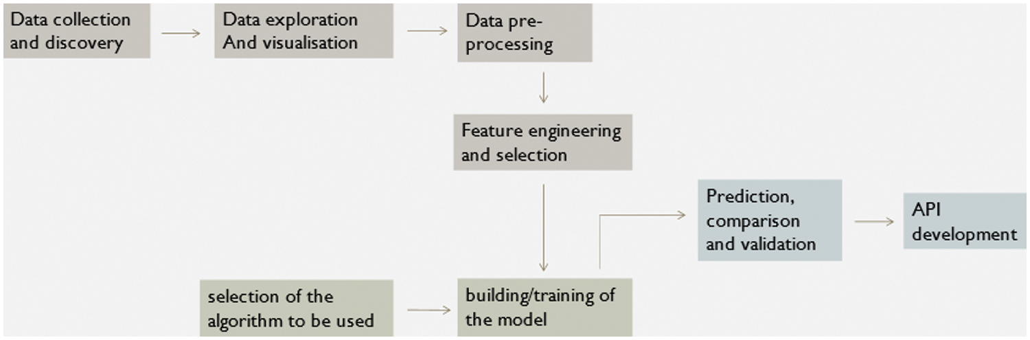
Figure 1: An outline of the study design in graphic form

2.1 Proposed Predictive Analytical Model

This section introduces the proposed convolutional neural network model, describes the model training technique, and discusses the performance metrics used to judge the model's performance.

2.2 Structure of the Proposed Model

There are four layers in the CNN model we propose, namely the output layer, the flattened layer, the one-dimension convolutional layer, and the fully connected layers. The architecture of the suggested model is shown in Fig. 2.

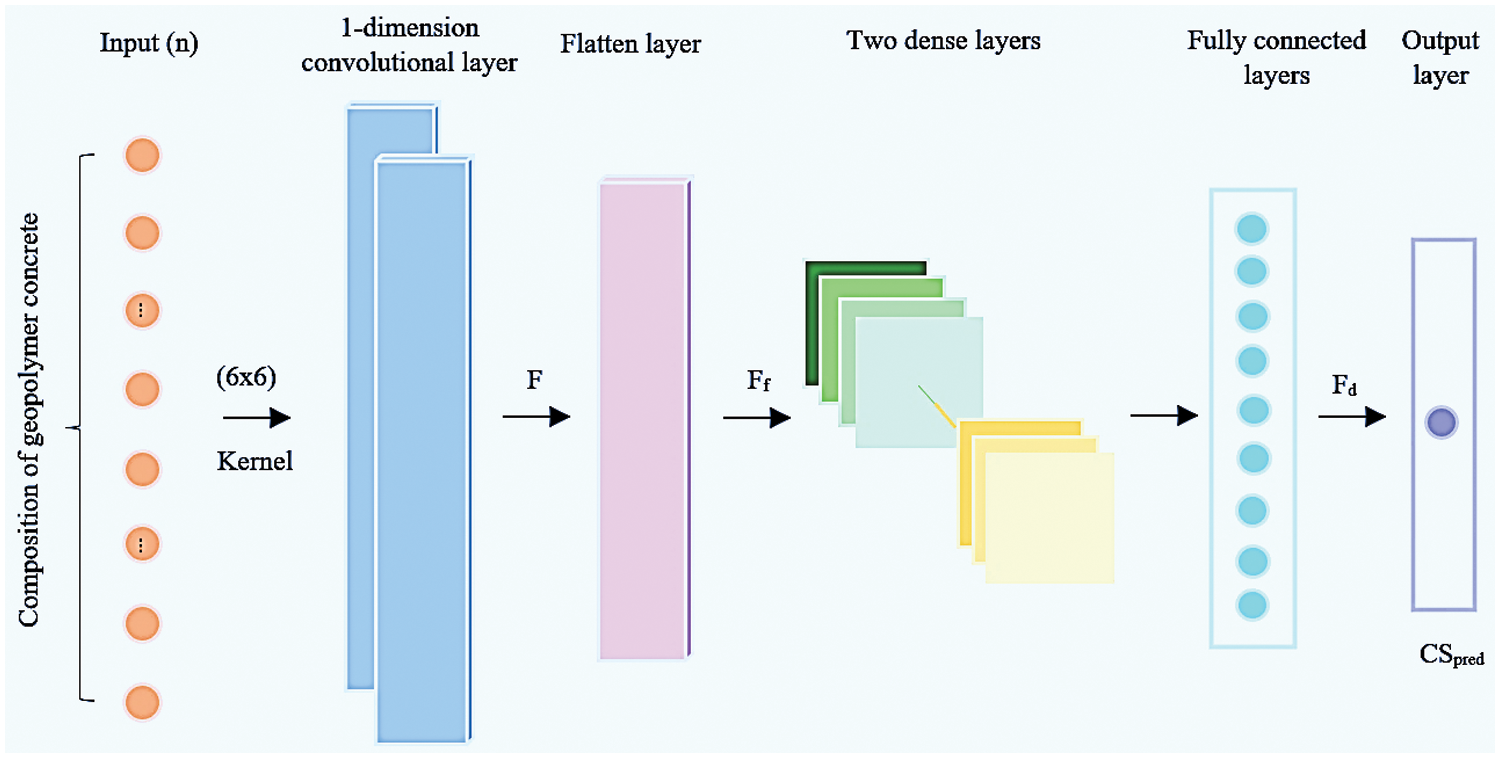
Figure 2: Illustration of the proposed CNN model’s architecture

2.2.1 The One-Dimension Convolutional Layer

This layer is primarily in charge of collecting the connections between input parameters using multiple convolutional kernels (the value of which is indicated by p). By utilizing multiple kernels, the model is able to pick up as many trends as feasible and look into further ways to enhance compressive strength forecasting. Each convolutional kernel slides across the entire input feature vectors with a particular stride u for each slide, calculating a weighted sum over all the q components the kernel covers for each slide. The values used for p (no. of convolution layer kernels) and q (dimension of the kernel) are discussed further. The value of u is set to 1 to allow the kernel to discover as many locally existing patterns as feasible, as bigger numbers can result in the kernel losing too much information and slipping through too many features. Within the convolutional kernel, the RELU (rectified linear activation unit) function functions as the activation function. RELU was chosen because the needed compressive strength is a positive real number and RELU can separate negative interim calculation results that influence the outcome. Fig. 2a illustrates the RELU function. For the specified input feature vector z with n dimensions, this layer's final output for the Pth convolutional kernel is shown below:

F=[f1,……,fp],F∈R(n−q+1)×P(1)

In Eq. (1), F is a set of feature vectors generated by p convolutional kernels. The size of the matrix is (n-q+1, P). This type of matrix holds the information from all the retrieved feature patterns that locally exist for an input z and can be used as a more edifying feature in succeeding layers.

2.2.2 The Flattening Layer

Matrix F is flattened into a 1-d feature vector. Later it passed to the fully connected layers to retrieve further hidden patterns. The flattened layer's corresponding feature vector Ff is calculated as follows:

Ff=[f1⋮fp],Ff∈R(n−q+1)×P(2)

2.2.3 The Fully Connected Layers

Because of the input parameters and compressive strength's extremely nonlinear relationships, only superficial patterns are present in the flattened vector Ff, making it impossible to infer compressive strength from it. To solve this issue, A deep latent feature vector is obtained by sending Ff across D number of fully connected layers in order to simulate and learn the appropriate non-linear connection. Each fully connected layer's intermediate results are calculated as follows, where dth fully connected layer has gd neurons.

Fd=[F1d⋮Fid⋮Fgdd],Fd∈Rgd,1≤d≤D(3)

Fid=RELU(∑j=1gd−1(wi,jd×Fjd−1))(4)

wid={wi,jd}j=1gd−1(5)

Here, for the ith neuron within dth fully connected layer, wid is an array of trainable weights which are denoted by wi,jd. The activation function chosen for this step is Rectified Linear Unit (RELU). The activation function chosen for this step is the Rectified Linear Unit (RELU) shown in Fig. 3a.

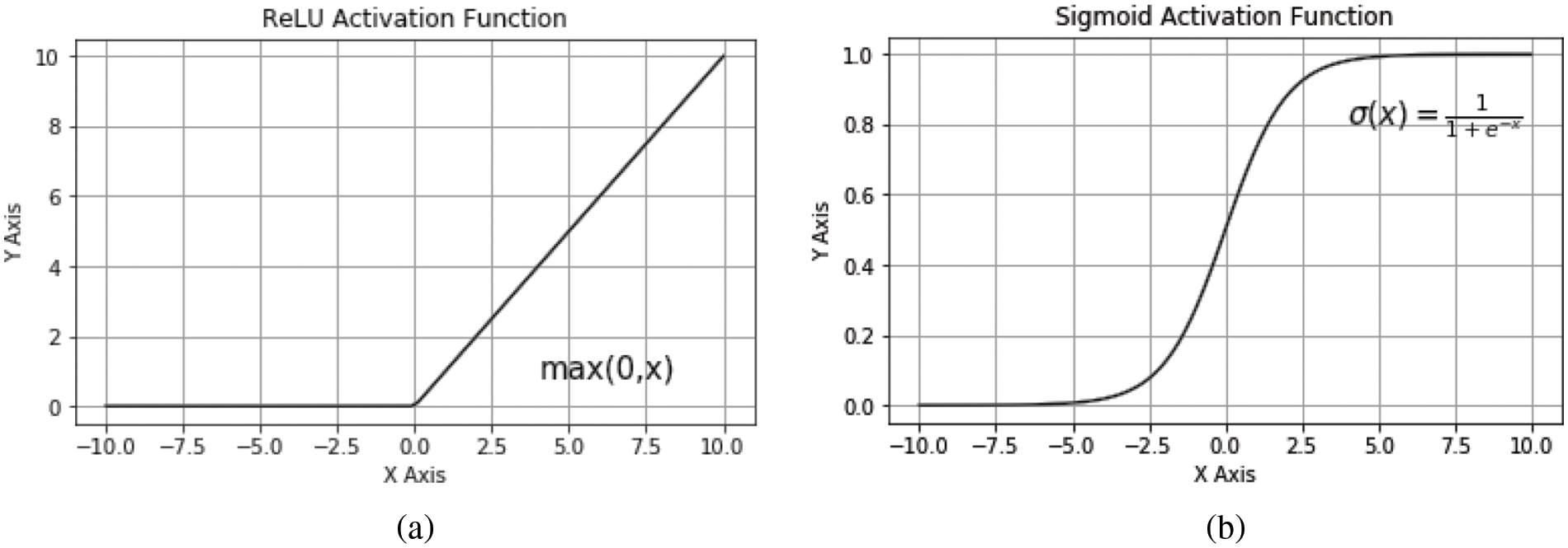
Figure 3: Illustration of activation function: (a) RELU activation function (b) Sigmoid activation function

2.2.4 Output Layer

The final compressive strength prediction is carried out by another fully connected layer with a sigmoid activation function. Fig. 3b illustrates the sigmoid activation function. The estimated compressive strength is calculated by:

CSpred=sigmoid(∑j=1gd(wj0×FjD))(6)

w0={wj0}j=1gd(7)

Here, w0 represents the output layer’s trainable weights. Because of the sigmoid function's unique properties, the estimated compressive strength (CSestm) values will be in the [0,1] range. Later, for model evaluation, by employing the normalizing function's inverse operation, these values are normalized to their actual scale.

2.3 Training of the Model

2.3.1 Loss Function

A binary cross-entropy loss function was utilized to calculate the loss generated during the prediction process between its real and estimated values. The sigmoid activation function, being the only function compatible with this loss function, was employed. In the following set of formulas, the loss value between real compressive strength values and estimated compressive strength values is determined as shown in the former expression. The latter formula in the set of formulas below is used to compute the overall loss by calculating the mean of individual loss Lz of every estimated value for the input z.

Lz=−CSreallog⁡(CSestm)−(1−CSreal)log⁡(1−CSestm)(8)

L=1N∑zLz(9)

To improve the model weights based on the above loss, Adaptive Moment Estimation (Adam) is utilized, which is one of the most frequently used optimizers. Adam's ability to asynchronously change learning rates for parameters has been proven to perform successfully in practice with the default configuration. The number of epochs E for learning and Adam’s dynamic rate of learning are two of the many hyperparameters, and optimal values of epochs are investigated and examined in the upcoming sections.

2.3.2 k-Fold Cross-Validation

Given that the division of training and testing databases and the arbitrary assignment of trainable weights can affect training and evaluation results, a cross-validation strategy is employed to train and evaluate the model rather than a fixed training-testing split. This method can minimize the impact of randomization and improve the visualization of the model’s predictive accuracy. The technique of k-fold cross-validation is a well-known method for assessing the performance of a machine learning algorithm on a database. The database is divided into k number of non-overlapping folds using the cross-validation technique of k-fold. One of the k-folds is chosen as the held-back test set, whereas the rest are utilized collectively as the training dataset. After fitting and assessing k models on k hold-out test sets, the average performance is provided. The most common choices for the value of ‘k’ are 3, 5, and 10, with 10 being the most frequently used value in many studies to evaluate models. This is because the research was conducted, and k = 10 was discovered to give a suitable trade-off between cheap computing cost and low bias in an assessment of model performance [12,13]. On the contrary, some researchers have also concluded that a model with 5 folds (k = 5) has also shown acceptable performance, particularly in saving time and tackling computational complexity. The question is what value of k to utilize for CNN model evaluation on the geopolymer dataset to attain the best possible performance. The approach chosen in this study to answer this question was to compare the performance of the model, using a certain database, for varying k values. k’s value would range from 2 to 30.

2.3.3 Setting of the Hyperparameters

The proposed model’s hyperparameters are as follows: kernel dimension; number of neurons in the completely connected layer; number of kernels in the convolution layer; number of fully connected layers; training epochs, learning rate, and the activation function. Because a hyperparameter governs the learning process, its values directly affect other model parameters like biases and weights and thus how well the model works. The convolution layer’s number of kernels was set to 32, the number of fully connected layers was 2, the kernel dimension to 6 the number of neurons in the 1st fully connected layer was 128 and the 2nd was 64, and the learning rate was set to 0.01, and Rectified Linear Unit (RELU) was selected as the activation function for the fully connected layers. These values of hyperparameters were chosen on the basis of previous work which used a similar set of hyperparameters whereas the rest were decided by utilizing a trial-and-error approach. The number of times the learning algorithm will loop through the entire training dataset is determined by the hyperparameter known as the training epoch. Any positive integer between one and infinity can be chosen. The most typical values are 10, 100, 500, and 1000. The training epochs were not chosen based on studies; three empirical values were chosen for them, which were 500, 200, and 5000, and then, utilizing the cross-validation technique, the performance of the model under all possible combinations of training epoch value and k-fold value as mentioned in the previous section was studied. In total, 87 configurations were tested on each dataset, and the combination that produced the least average root mean square error was considered the optimum combination.

2.4 Performance Metrics

Four performance metrics were used to assess how effectively the proposed CNN model functions, which are, the mean absolute error (MAE), mean absolute percentage error (MAPE), correlation coefficient (R), and root mean square error (RMSE). R determines whether the real and estimated compressive strength values have a linear relationship. While Mean Absolute Error takes the square of the errors, RMSE provides an error measure in the target variable’s unit. Instead, it just estimates the absolute value of the errors and then averages them. MAE, like RMSE, does not square the units, making the findings more interpretable. MAPE expresses the percentage of real and estimated values’ differences. By presenting the mistake as a percentage, it provides a better grasp of how far off the forecasts are in relative terms. In general, a larger R-value suggests better model prediction performance, while a lower value indicates better performance for RMSE, MAE, and MAPE. The following is the calculation formulas for the four indicators mentioned above:

R=∑i=1N(yi−y¯)(y^i−y~)∑i=1N(yi−y¯)2(y^i−y~)2(10)

RMSE=∑i=1N(yi−y^i)2N(11)

MAE=∑i=1N|yi−y^i|N(12)

MAPE=∑|yi−y^i|yi×100N(13)

In the above-mentioned formulae, yi and y^i are the real and predicted compressive strengths in a database. Correspondingly, y¯ is the average value of the real strength value, y~ is the average value of the estimated strength value; and N is the entire data quantity.

3  Materials and Methods

3.1 Data Acquisition and Data Pre-Processing

A dataset was acquired from the work of Toufigh et al. [33]. In their study, data was collected from papers published from the years 2000 to 2020 [38–41]. This dataset contained one hundred and sixty-two mixed-design values. Table 1 enlists the influential parameters affecting the 28-day compressive strength of fly ash-based geopolymer.

By studying the fly ash constituents, it could be deduced that the fly ash used in all these mix designs had a low amount of calcium oxide, which makes it class F fly ash. Table 2 describes the data in the data frame concerning the concrete studied in this inquiry. Each column’s description contains details such as std (standard deviation), count (number of non-empty values), mean (average value), 75% (75th percentile), 50% (50th percentile), 25% (25th percentile), and max (maximum value) and min (minimum value) with percentile indicating the proportion of values that are smaller than the stated percentile.

The data frame was also examined for any null values, and it was determined that no null values existed. While analyzing the data, outliers were discovered in a couple of the features. Although it is said that outliers may cause elevated error rates, no attempt has been made to delete them since some scholars believe that their removal may result in bad outcomes [42]. One of the distribution visualization techniques used to comprehend the distribution of the variables was a combination of kernel density estimate (KDE) plots and histograms. Distribution visualization techniques provide answers such as an observation’s range, central tendency, degree of skewness in one direction, etc. KDE plots provide numerous benefits: the data’s most important aspects are easily discernible (skew, bimodality, central tendency). However, there are times when KDE fails to accurately display the underlying data. This is due to KDE’s logic assuming that the underlying distribution is continuous and boundless. If there are close observations (for instance, minimal non-negative values of a variable), the KDE contour might extend to unrealistic values. One of the most prevalent methods to display a distribution is with a histogram. A histogram is a bar graph in which the axis indicating the data variable is segmented into distinct segments. The height of the corresponding bar indicates how many observations occurred inside each segment. The KDE shows that there are surges near numbers, whereas the histogram shows a much more cluttered distribution. As a result, as a compromise, these two approaches can be combined as depicted in Fig. 4.

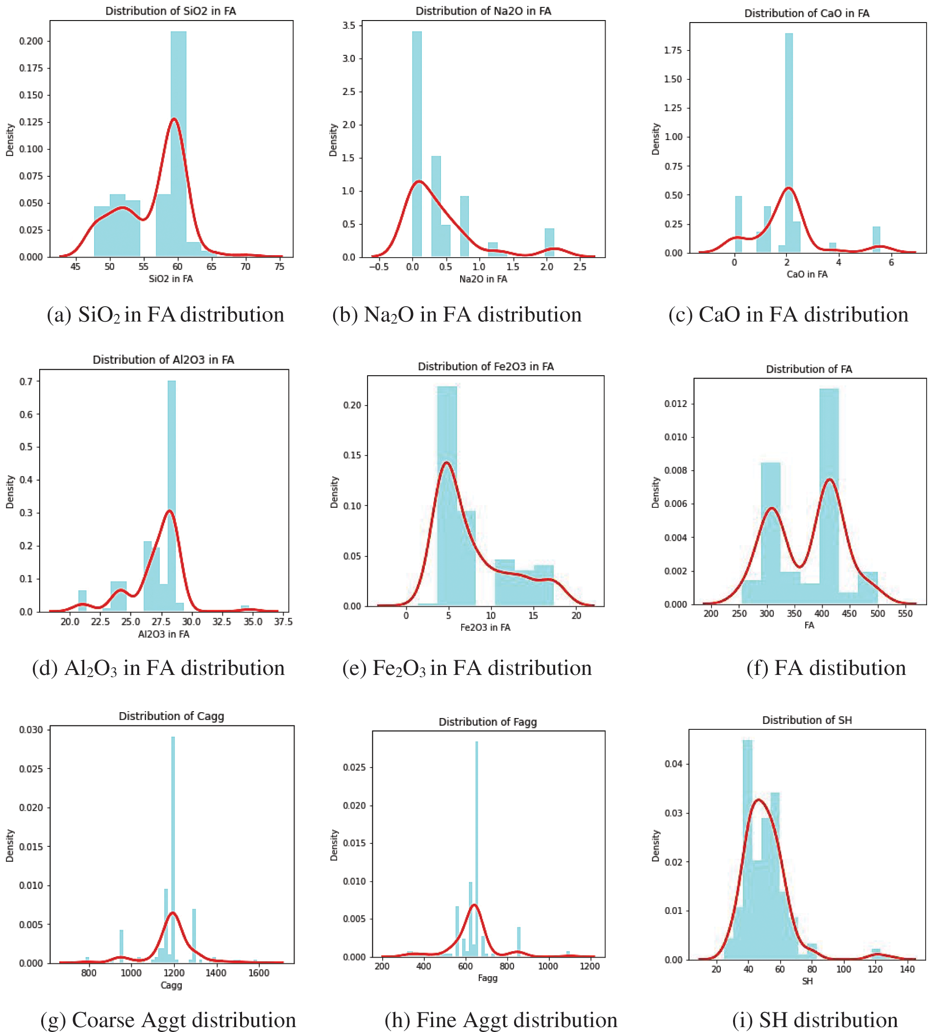
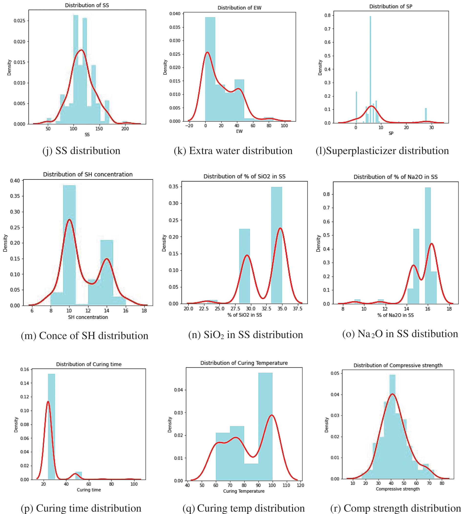
Figure 4: KDE distribution of various features the GPC dataset

Features such as silicon dioxide in fly ash, the content of fly ash, and curing temperature were symmetric negatively. Positively symmetric sodium silicate solution and sodium hydroxide concentration Aluminum dioxide in fly ash, coarse aggregate, and the percentage of silicon dioxide in sodium silicate curing temperature was moderately negatively skewed. Fine aggregate, extra water, and compressive strength were moderately positively skewed. The percentage of silicon dioxide in sodium oxide seemed highly negatively skewed. Sodium oxide in fly ash, calcium oxide in fly ash, iron oxide in fly ash, sodium hydroxide solution, superplasticizer, and curing time were highly positively skewed. Fig. 5 is an illustration of the Spearman correlation matrix.

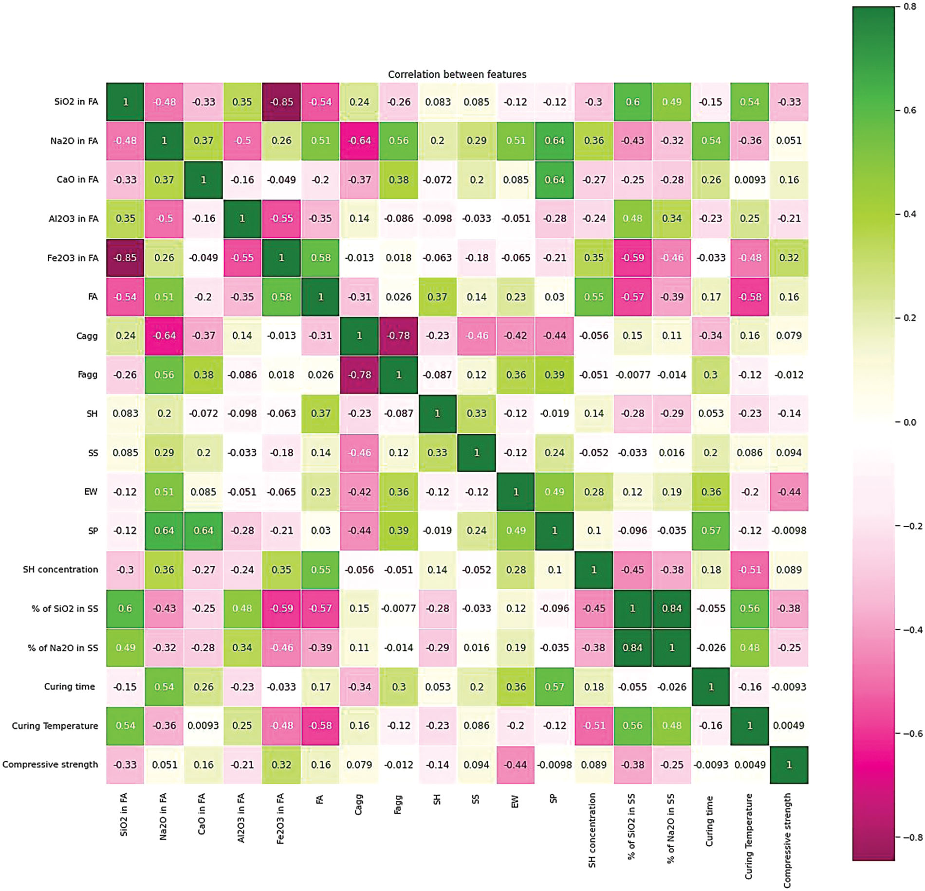
Figure 5: A heatmap of Spearman correlations for the features of the acquired GPC datasets

The relationship between each of the possible value pairings is depicted in the matrix. It is an effective tool for analyzing large volumes of data and discovering and visualizing data trends. The correlation matrix is made up of columns and rows, each focusing on a different attribute. The columns and rows are all arranged in the same order. The correlation coefficient is found in each cell of a table. The results confirm that the correlation between the percentage of silicon dioxide in sodium silicate and the percentage of silicon dioxide in sodium oxide was positively and highly related, whereas the correlation between coarse aggregate & fine aggregate and iron oxide in fly ash & silicon dioxide in fly ash was negatively and highly related, and the other correlation was not significant enough.

3.2 Input Parameters

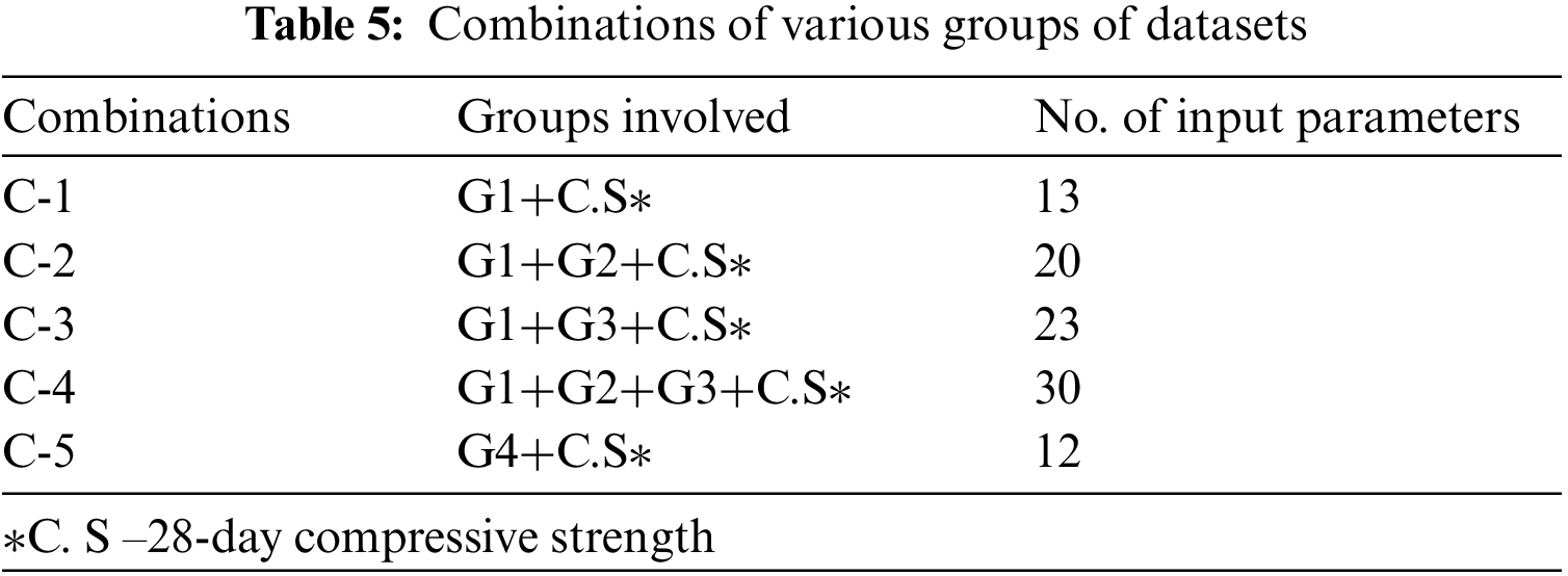
Some studies claim that using a large dataset formed of key input features to train a model outperforms one trained with fewer input parameters. Some also say that explainable features, i.e., attributes grouped by engineers based on their influence on the development of concrete strength that is already known or potentially discoverable through research, are well-suited for prediction. Input feature groups were created for this study. While some of the input features were engineered from the initial features, others were taken directly from Table 1.

Group 1: Features with a well-known and significant impact on geopolymer concrete's strength.

Group 2: Features pertaining to fly ash’s composition.

Group 3: Ratios utilized by various researchers to predict geopolymer concrete's strength.

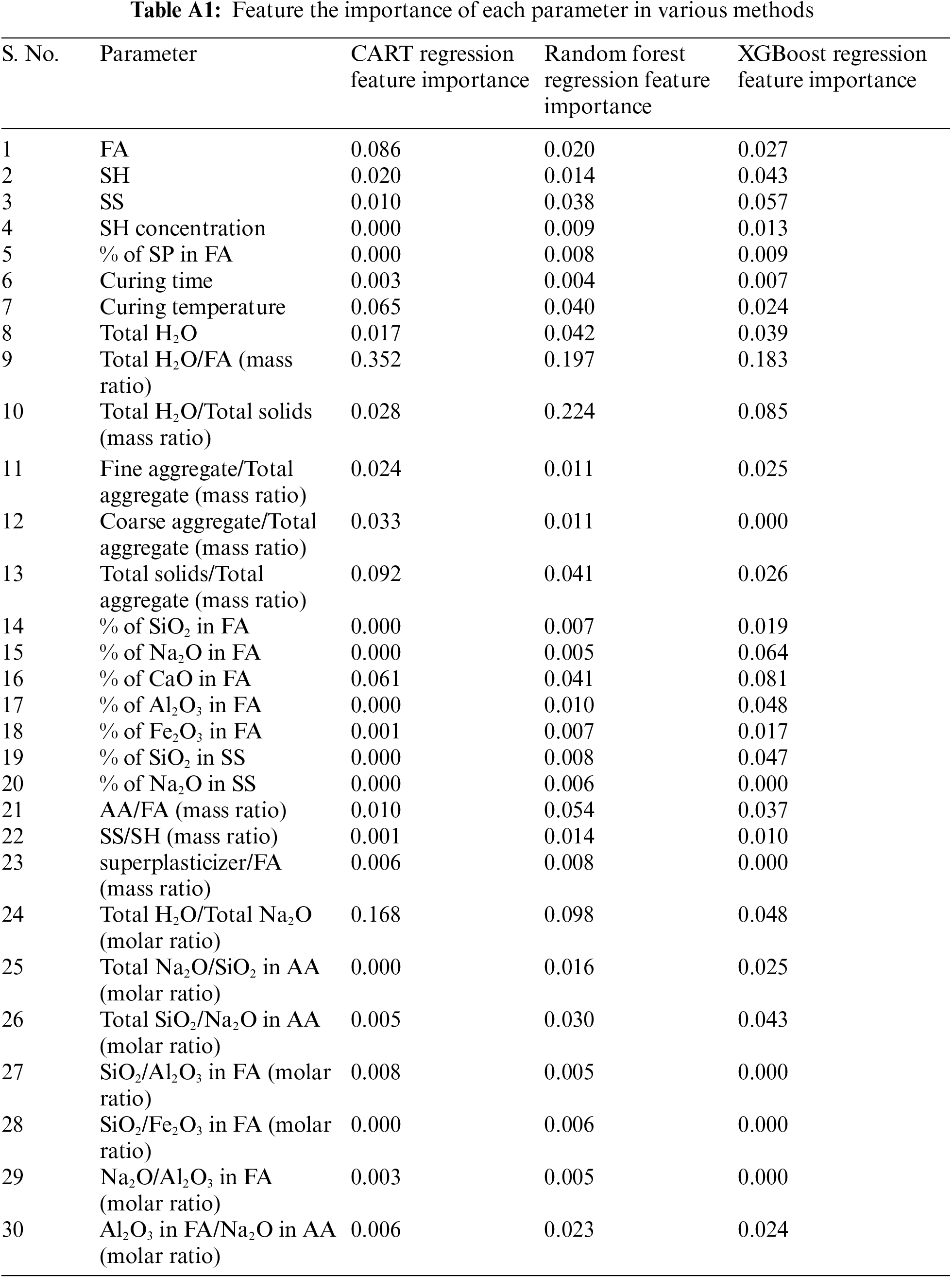
Group 4: The top 12 features from groups 1, 2, and 3 that performed well across three feature-importance methods i.e., Random Forest Regression Feature Importance, CART (Classification and Regression Tree) Regression Feature Importance, and XGBoost Regression Feature Importance. The scores of these methods for every feature can be found in Appendix A. Scores in feature importance techniques are assigned to input features chosen for the predictions that indicate their relative importance in predicting. They help to highlight the relevance of data, provide insight about the model being used by conveying which features are most important for an efficient prediction, and better the model by eliminating features with low scores which indirectly help fasten the process and enhance the process. Table 3 shows various input parameter groups of datasets. Based on feature importance, the input parameters that are bound to greatly influence the prediction are grouped as G4 and tabulated in Table 4.

Table 5 shows combinations of various groups of datasets. The model was trained using each of these combinations, and its performance for various epoch values and k values was assessed. Combinations’ performance was judged based on error-related performance metrics, mainly root mean square error (RMSE).

3.3 Generality of Model

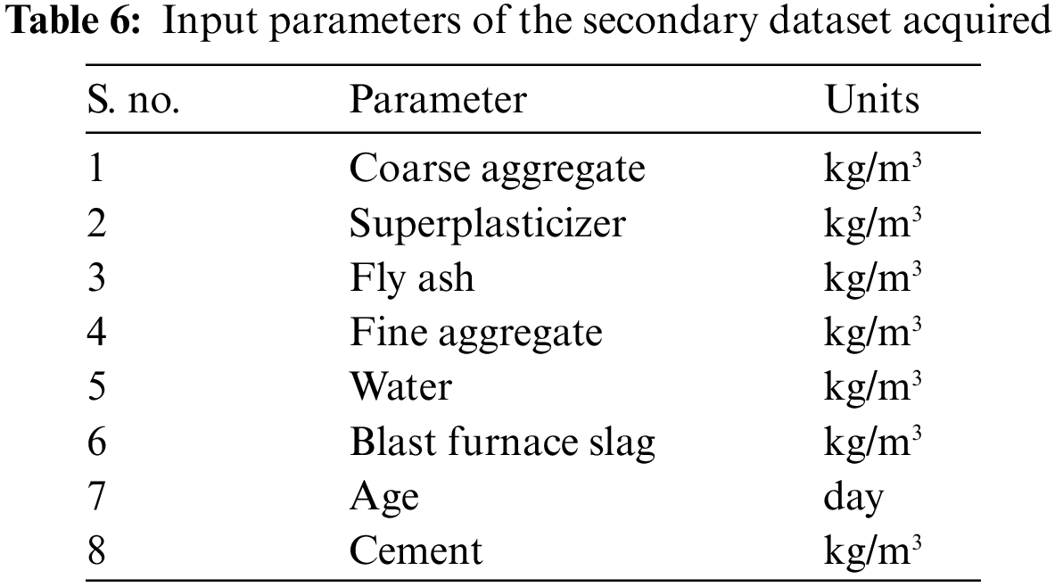
To examine the adaptability of the CNN model, a secondary dataset was acquired and used in the model. This dataset, generated through the work of I.C. Yeh of the University of California, 1030 compositions and their corresponding concrete strength values for high-strength concrete mixes. Many researchers have used this dataset to study the data in various ways and test out new machine learning techniques. Table 6 enlists the input parameters for estimating high-strength concrete mixes' compressive strength.

4  Results and Discussion

4.1 Influence of No. of k-Folds and Epochs

All the combinations mentioned in Table 5 were analyzed in the CNN model for each of the 87 combinations mentioned previously. Fig. 6 represents k-fold cross-validation results for combination 1 for all the epoch values.

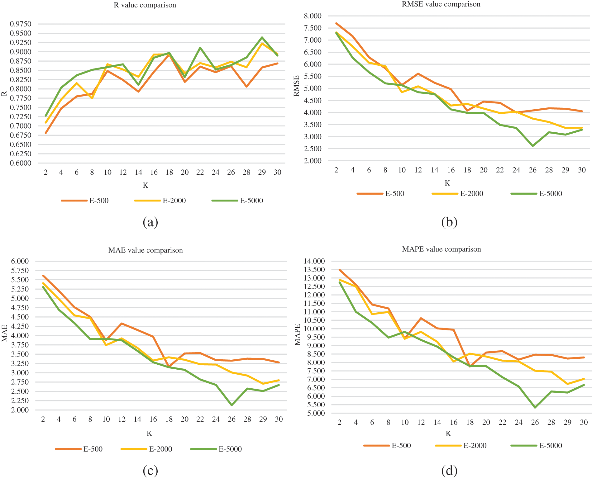
Figure 6: k-fold cross-validation results for the combination 1 for all the epoch values: (a) Variation of R (b) Variation of RMSE (c) Variation of MAE (d) Variation of MAPE

Each epoch value has been represented in each graph by a distinct color. Fig. 5a depicts the variation of the correlation coefficient (R) across k values for the three epoch values, demonstrating and deducing that the R-value increases as the k-fold value increases, and the variation of R across k values follows the same trend for all three epoch values. Among the three, the epoch value of 5000, shows the highest R-value for the k-fold value of 29. Overall, the epoch 5000 trend has the highest R-value across all folds. Figs. 5b–5d depict the variation of root mean square error (RMSE), mean absolute error (MAE), and mean absolute percentage error (MAPE), for the chosen 3 epoch values across k values. All three show that the combination which was analyzed for 26 k-folds produced the least amount of error for the epoch value of 5000. Finally, we can deduce that the optimal value of the k-fold lies in the range of 25 to 30 when the range is considered 2 to 30, and that this combination performs better when the epoch value is 5000. Fig. 6 illustrates the variation of the RMSE value of each fold when the dataset of combination 1 was analyzed in the CNN model for 5000 epochs and 29 k-folds. The average RMSE value for this attempt, 3.083, is highlighted at the end, as shown in Fig. 7.

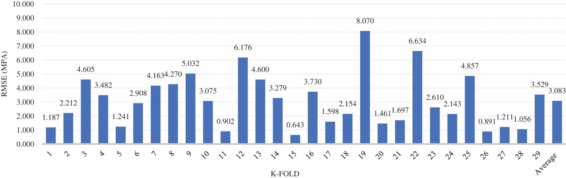
Figure 7: k-fold cross-validation results for 5000 epochs and 29 as the k value for the combination 1

Also, it was observed that the computational time for combination 4 was the highest since it had the most input parameters as mentioned in Table 5. This also applied to the increasing number of folds or epochs.

4.2 Influence of Input Parameter

As mentioned in Section 3.3, the effects of the numerous input parameters and their variety were studied. As listed in Table 5, the 5 combinations of input parameters were considered and analyzed in the CNN model for epoch values of 500, 2000, and 5000 for k-fold values ranging from 2 to 30. Table 7 depicts the performance of each combination of datasets for a randomly selected combination of epoch and k-fold value and the order of precedence.

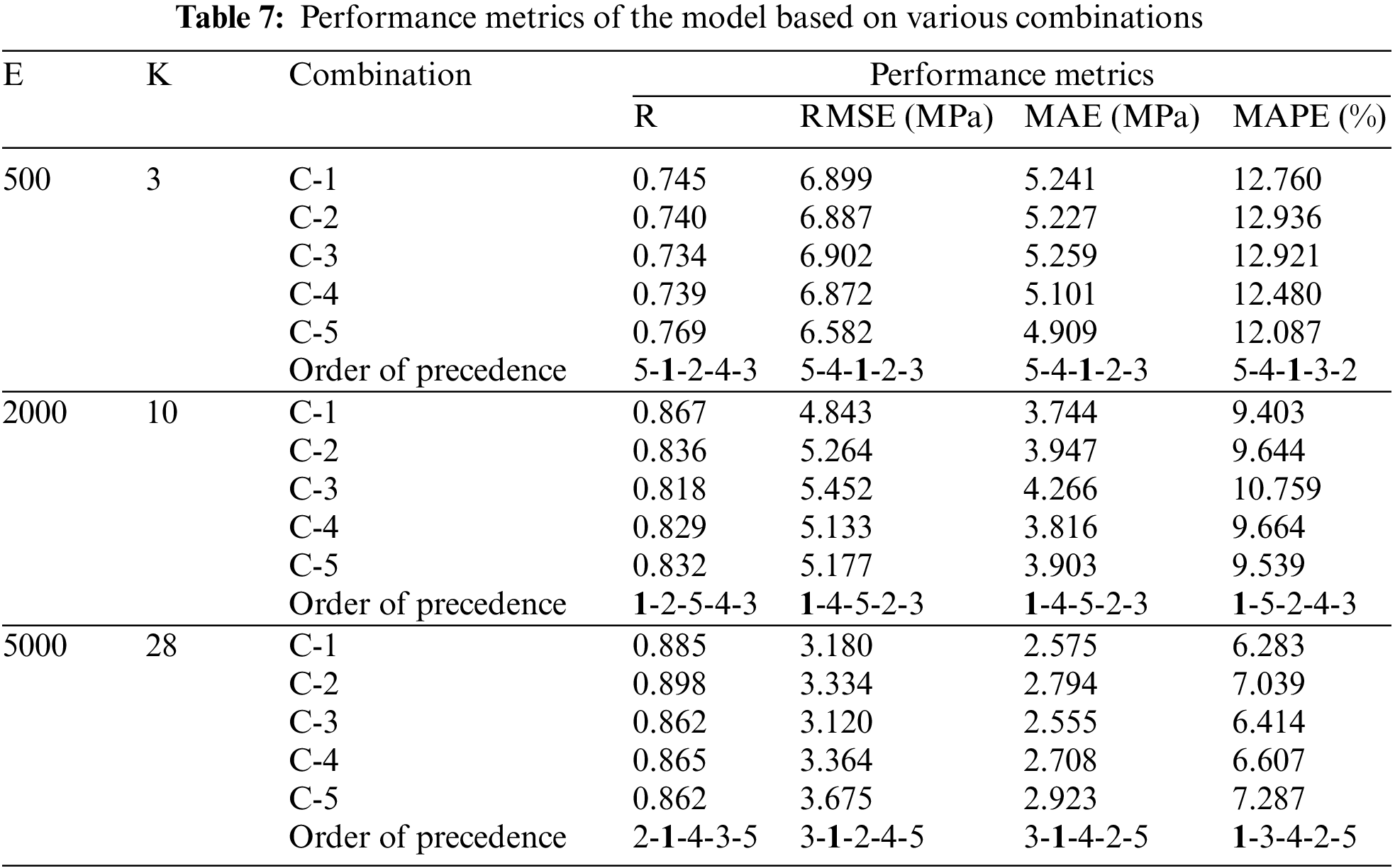
The results convey that combination 1 outperforms the others. The performance metrics of combination 1 improved as the epoch and k-fold values increased. Apart from that, combination 5, which consisted of parameters chosen based on feature importance, performed inconsistently over the range of epoch and k-fold values considered. Its performance was depleted as k-fold and epoch values increased. From studying the performance of each combination in terms of the influence of the number of variables, in agreement with the results of De-Cheng Feng [43], it can be deduced that as the model's performance depletes the number of variables increases. To summarize, it could be said that the important parameters in Group 1 influence the model to a large extent compared to other groups, such as Group 2 and Group 3, which contain a composition of fly ash and alkali activators and various ratios pertaining to the components of the concrete mix. Also, the novel approach of building a group of input parameters with the help of feature importance did not pan out as a significantly good result, as the performance of that combination performed inconsistently as mentioned before.

A learning curve uses experience to measure changes in learning performance over time. It indicates how well the model learns when plotted against the training dataset and how well it generalizes when plotted against the validation dataset. Models are evaluated and selected based on model performance. B. Accuracy. The optimization curve is calculated according to parameter optimization. B. You incur losses. Loss curve behavior was examined for epoch values of 50, 100, and 200 and k-fold values of 5, 10, and 25. It has been observed that the learning rate improves as the epoch value increases because the loss decreases faster with increasing epoch value. When a higher k-fold value was chosen, the loss value quietly decreased after each epoch.

4.3 Comparative Study

4.3.1 Performance Evaluation

A comparative study was done where the performance metrics of various traditionally used models were compared to the CNN model for the dataset of combination 1. Other than the CNN model, various models were built, such as the Random Forest regression model, Decision Tree Regression model, Linear Regression model, Ridge Regression model, Gradient Boosting Regression model, AdaBoost Regression model, and an ensemble model (containing the aforementioned models). Except for the CNN model, all the models divided the dataset in a 9:1 ratio, with 90% of the dataset used for training and 10% utilized for testing. This ratio was chosen due to the work of Hamza Imran, who had deduced from his work that the 9:1 ratio as the train-test split ratio would produce the best results [30]. Table 8 presents the performance of each of the models, which concludes that for this dataset, the CNN model outperforms the other models as well.

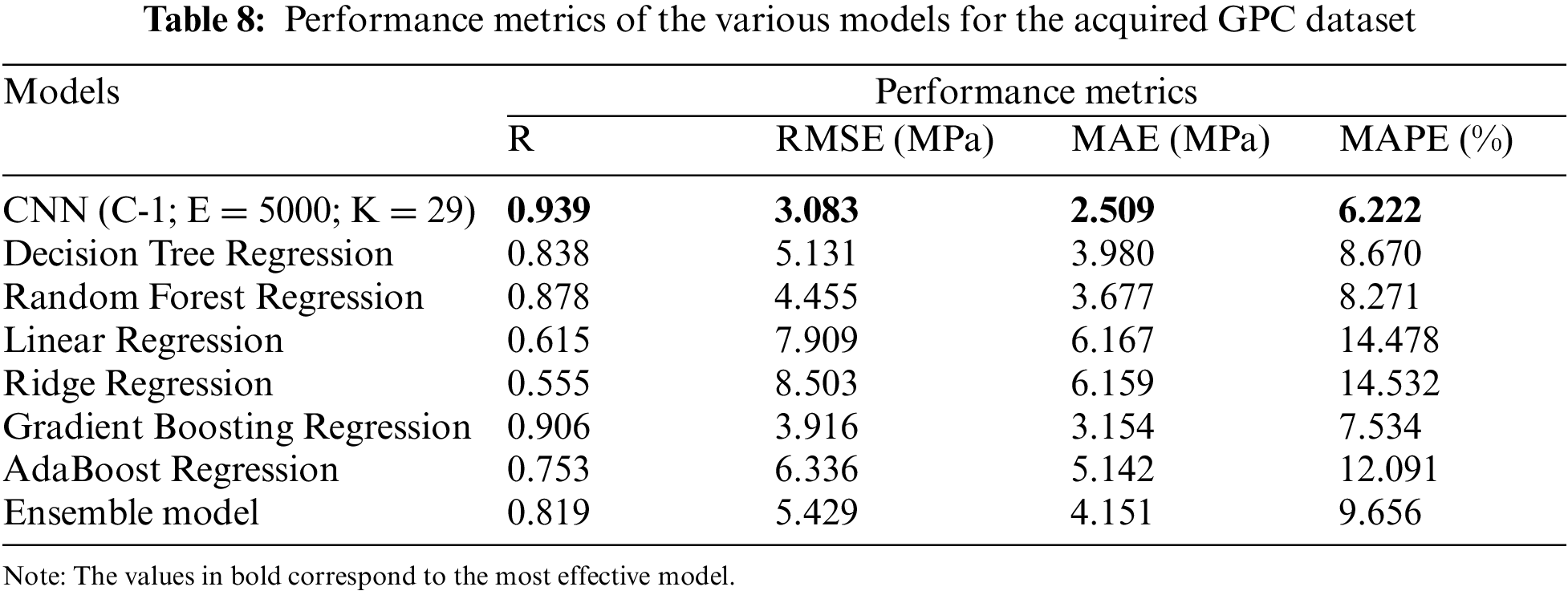
The gradient-boosting regression model seemed to have performed much like the CNN model. Models such as ridge regression, linear regression, and AdaBoost regression performed the poorest. To check the generality of the CNN model as mentioned in Section 3.3, the above-mentioned process was done with the secondary dataset acquired. Table 9 depicts the performance of each of the models, which concludes that for this dataset, the CNN model outperforms the other models as well.

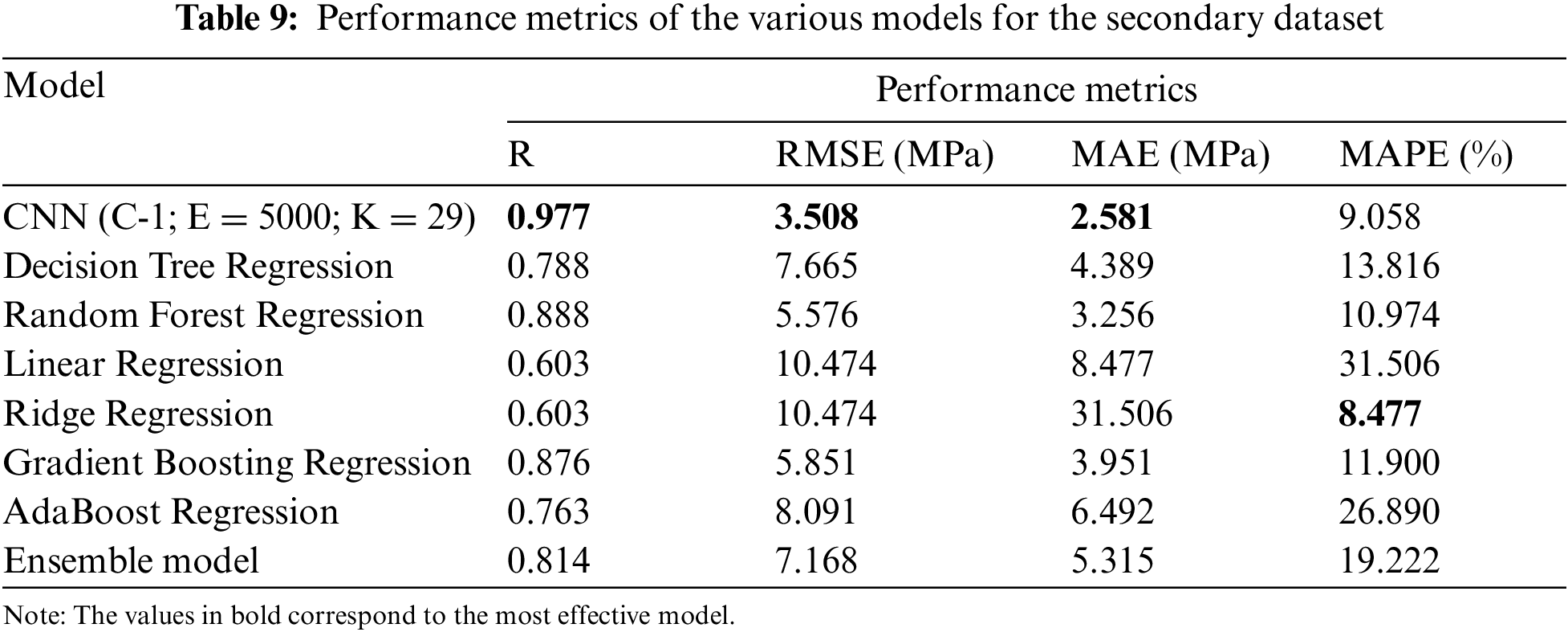
The gradient-boosting regression model seemed to have performed very similarly to the CNN model. Models such as Linear regression, Ridge regression, and AdaBoost regression performed the poorest.

4.3.2 The Score Analysis

The technique of score analysis was applied to compare the performance of various models in a simple manner. Using this technique, the model is assigned a score of x. When models are placed in descending order depending on their performance in each metric, x represents the position obtained by each computational model. The maximum value of x would be the total number of computational models used in the performance comparison (maximum value of x is equal to 8 here), which would be assigned to the model with the best performance based on that metric, and the minimum would be 1, for the model with the worst performance in that particular metric. Each computational model would acquire a separate score for its performance for each evaluation metric, i.e., R, RMSE, MAE, and MAPE. Following that, the total score corresponding to each of the models is derived by adding their separate scores [44,45]. The information regarding the score analysis performed on the models has presented in Table 10.

The results suggest that the CNN model used in this study gained the best score of 32. Other models whose performance almost matched the performance of the CNN model were the Random Forest Regression model, Gradient Boosting Regression model, and Decision Tree Regression model. The Ridge Regression model performed the least among all, with a score of 5. Fig. 8 illustrates the findings of the score analysis as a radar diagram. It easily demonstrates the precedence of the CNN model.

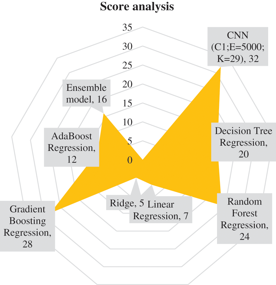
Figure 8: Visualization of score analysis using a Radar diagram

4.3.3 Generality of the Model

To check the generality of the CNN model, the above-mentioned process was repeated with the secondary dataset acquired. Table 11 depicts the performance of each of the models, which clearly concludes that the CNN model performs better than the rest of the models for this dataset as well. This result indicates the CNN model's consistent efficacy and generality in forecasting the compressive strength of not just geopolymer concrete but also high-performance concrete.

4.3.4 Predictability

To test the predictability of the model, the true values and the predicted values were compared. As shown in Fig. 9, it was found that the percentage variation between both ranges from 0.30% to 4.84%. Also, the difference in the values did not exceed 2.16 MPa. Fig. 9 is a software screenshot showing the output true and anticipated values.

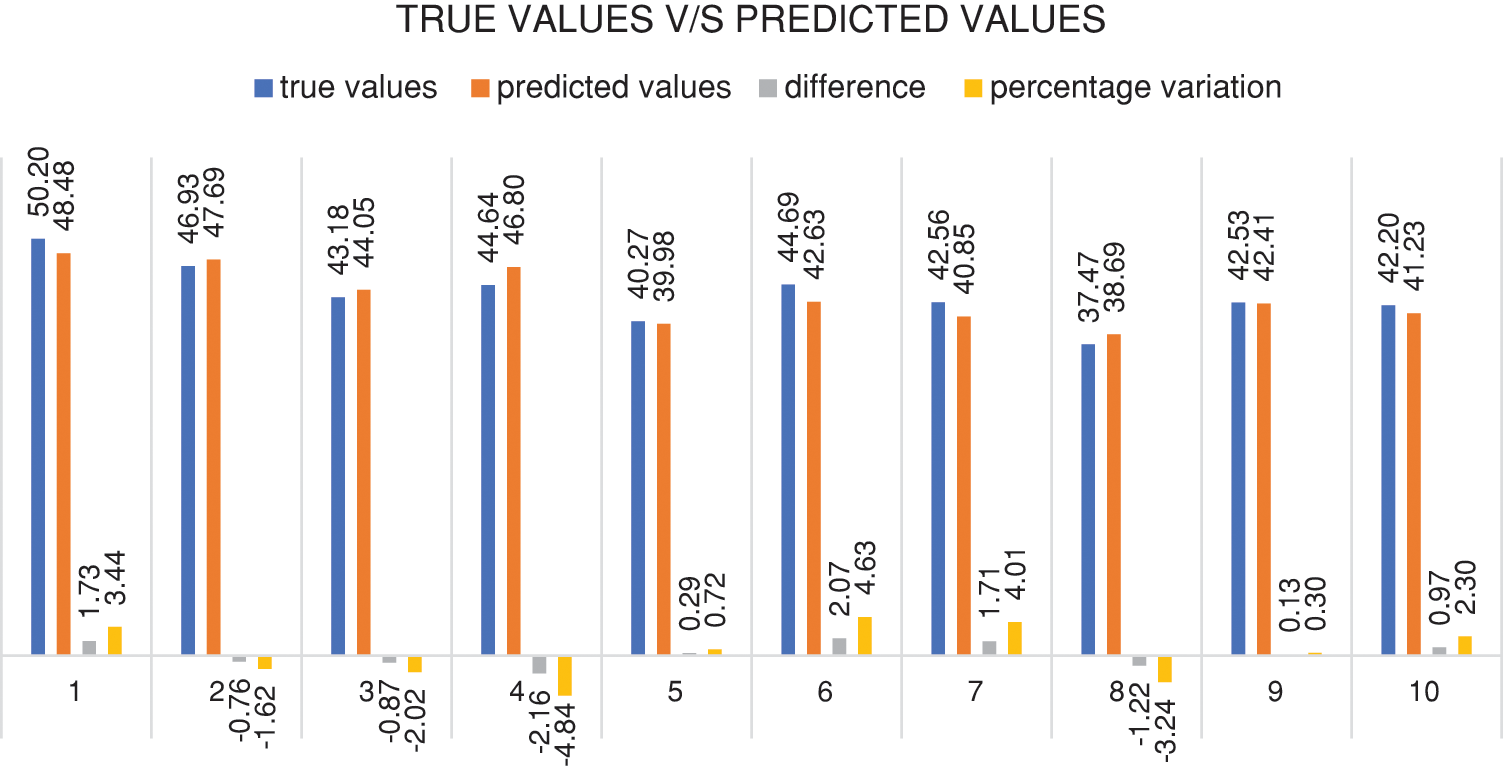
Figure 9: Illustrates true values vs. predicted values

4.4 Loss Curve

A loss curve was plotted to understand the training process and the way the convolutional neural network learns the data and optimizes itself. The loss (calculated as mentioned in Section 2.2.1) was plotted across every epoch of the data set of combination 1, which was trained with the k-fold value of 29 and for 5000 epochs. The advantage of plotting loss across epochs rather than every iteration or fold is that loss will be calculated for every data point instead of producing a loss value for a subset chosen in that fold. The curve's form in Fig. 10 represents a high learning rate since the loss seemed to decay fast with the increment in epochs.

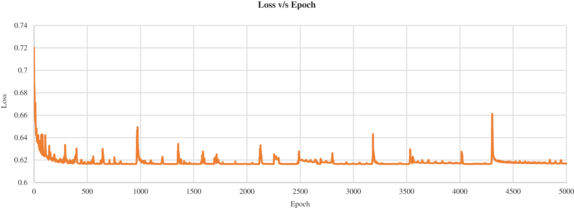
Figure 10: Representation of loss against epochs

4.5 Effect of Parameters on Compressive Strength

This section examines the numerous trends and interactions between variables. Fig. 11 shows scatter plots generated among different features. The correlation between fly ash content and its corresponding compressive strength is depicted in Fig. 11a. The addition of fly ash appears to have a small favorable effect on compressive strength. Strength appears to be strong in the zone where fly ash concentrations range from 400 to 450 kg/m3. Fig. 11b depicts the relationship between sodium hydroxide concentration and compressive strength. The greatest compressive strength is found at 14 M. This result is consistent with previous work [2]. Fig. 11c shows the relationship between the percentage of superplasticizer in fly ash and compressive strength. It was discovered that there is no substantial change in strength when the percentage changes. However, the maximum value is attained at a rate of between 1% and 2%. Fig. 11d depicts the influence of curing temperature on compressive strength. There is no discernible trend across the curing temperature range. Fig. 11e depicts the variation in total water and compressive strength. Water harms compressive strength, as was recognized. This result is consistent with previous work [2]. The correlation between compressive strength and total water/total solids is shown in Fig. 11f. It was obvious that as the ratio increased, the strength diminished. This outcome is in line with an earlier study [5]. The correlation between compressive strength and SS/SH (mass ratio) is shown in Fig. 11g. It has been observed that as the ratio rises, so do the strength levels. Fig. 11h depicts the variation in total water, total sodium oxide, and compressive strength. As stated in previous studies, strength appears to decrease as the ratio increases [4,5]. The correlation between total sodium oxide and silicon dioxide in the alkali activator and compressive strength is shown in Fig. 11i. It was found that compressive strength is slightly improved by raising the ratio. Fig. 11j depicts the influence of an alkali activator/binder (fly ash) on compressive strength. Agreeing with what was stated in the previously done work, as the ratio increases, the strength decreases [4]. It appears to be greatest when the ratio is between 0.3 and 0.4. Fig. 11k depicts the variation in total water/fly ash (mass ratio) and compressive strength. The strength of the concrete rapidly decreases as the ratio rises. This result is consistent with previous work [2]. Fig. 11l depicts the variation in total solids/total aggregates (mass ratio) and compressive strength. Some of the highest values are found to be in the region of 0.25 to 0.3 of the ratios. The influence of the percentage of silicon dioxide and aluminum dioxide on the compressive strength of the concrete mix is represented in Figs. 11m and 11p, respectively. From the figures, it is concluded that the strength slowly decreases while the percentage of dioxides increases. The influence of the percentage of calcium oxide and ferric oxide on the compressive strength of concrete mix is represented in Figs. 11o and 11q, respectively. Both indicate that the strength increases with the percentage of the oxides increases. The correlation between compressive strength and sodium oxide percentage in fly ash content is shown in Fig. 11n. When the amount of sodium oxide is around 0.4, the compressive strength appears to be at its greatest. There is no discernible pattern in their performance. The correlation between the curing time and the compressive strength is depicted in Fig. 11r. When the time is set to 24 h, the greatest value is seen.

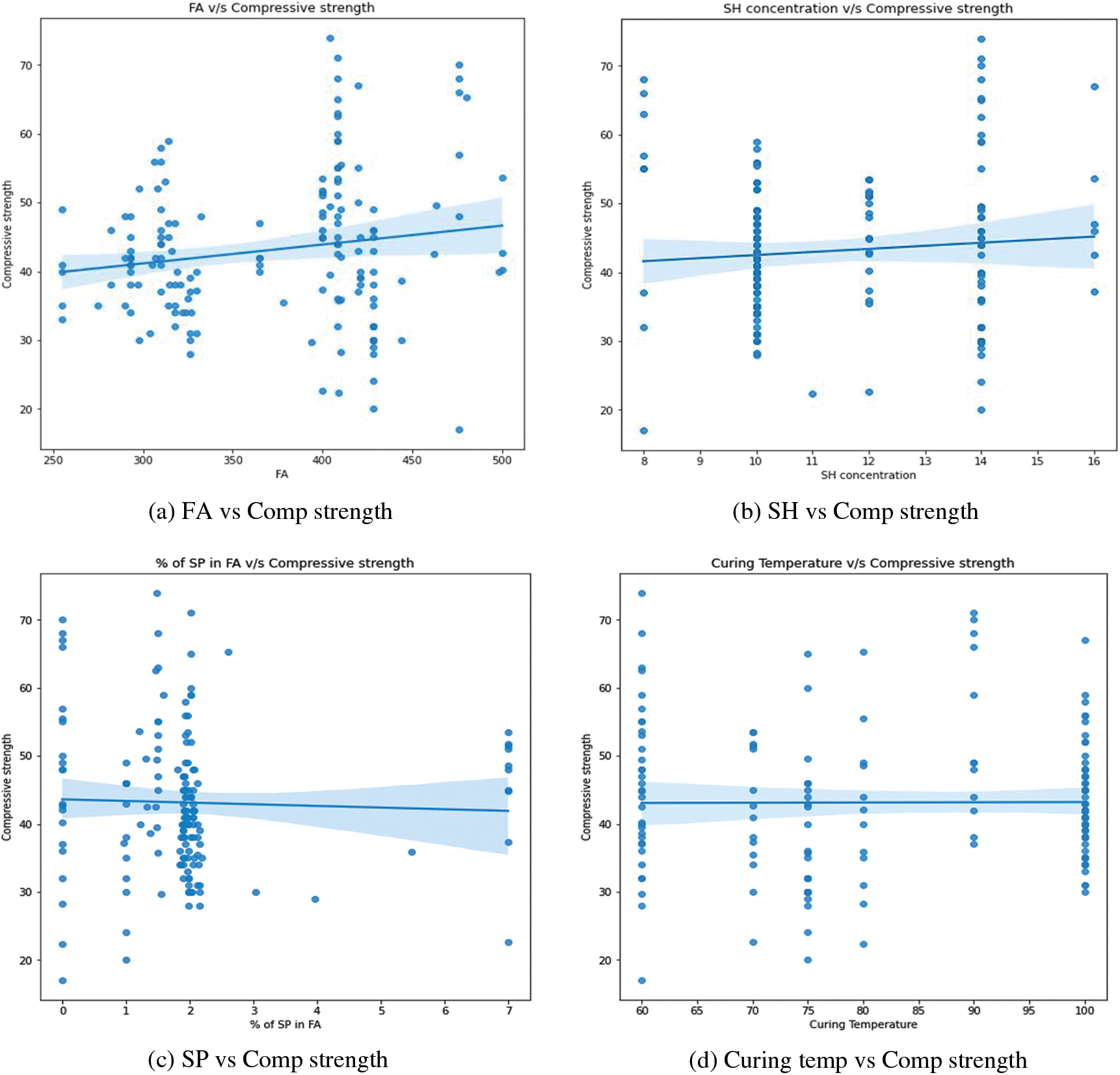
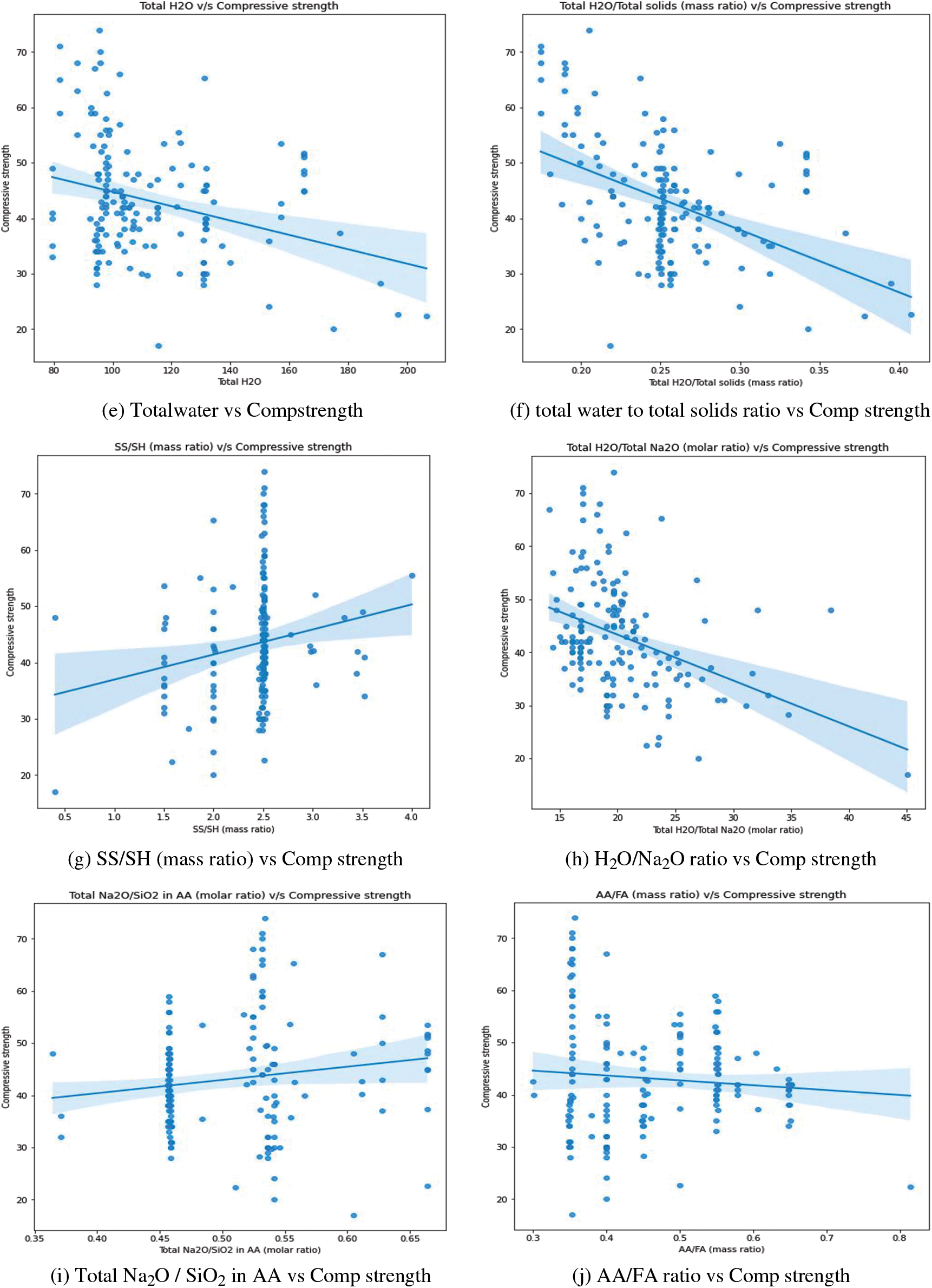
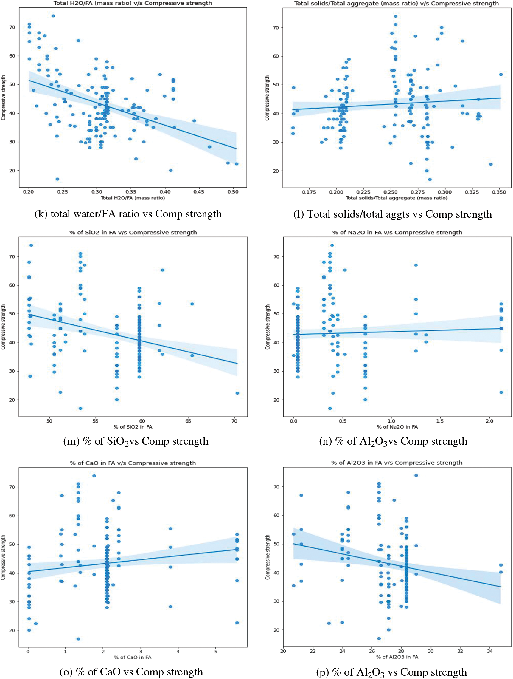
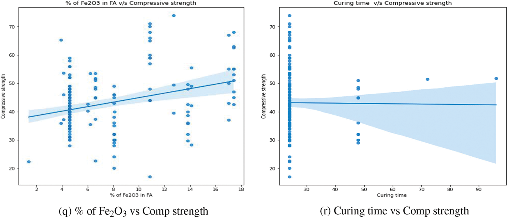
Figure 11: The influence of various features on compressive strengths

5  Summary and Conclusions

This work used an optimized deep learning model utilizing convolutional neural networks to solve the effectiveness and application challenges of current methods for forecasting geopolymer concrete's compressive strength. A dataset comprising the composition of 162 Class F fly ash geopolymer concrete mixes as well as 28-day compressive strength values were obtained. Using prior knowledge of each feature's influence on compressive strength as well as feature importance techniques, an ideal set of input parameters was carefully chosen. The optimal number of epochs (how many groups a certain dataset should be divided into) and the optimal value of k to run the k-fold cross-validation technique (the number of groups into which the data sample should be split) for the model that yielded the best results were determined through a process of trial and error. The performance metrics of this model were compared to different previously existing models for the obtained geopolymer concrete dataset as well as a secondary dataset (the high-performance concrete dataset) to evaluate the model's predictability and adaptability. The following points were made:

i)   In the analyzed geopolymer concrete database, the proposed model's R, RMSE, MAE, and MAPE were 0.939, 3.083%, 2.509 MPa, and 6.222%, respectively, indicating that the prediction error is reasonable and that the model can accurately forecast the compressive strength of geopolymer concrete. Compared to traditional approaches, the proposed model for predicting geopolymer concrete compressive strength has significantly lower error metrics. The difference between the true and anticipated values did not exceed 2,16 MPa, or 4.84%, which indicates the model's predictability is efficient.

ii)   It was necessary to adjust hyperparameters for the k-fold cross-validation technique, such as k (the number of groups into which each data sample should be split) and epochs (the number of times the training data was passed through the algorithm). The performance of the model was greatly influenced by the number of passes through the algorithm. In k-fold cross-validation, the optimal value of k was determined to be between 25 and 30 for all dataset combinations. The epoch value of 5000 performed best on all combinations despite the long computational time.

iii)   For epoch values of 500, 2000, and 5000 and k values ranging from 2 to 30, the algorithm was executed for five combinations of input parameters that were evaluated and analyzed in the proposed model. Combination 1, which is a collection of essential parameters, outperforms the others. As the epoch and K values increased, so did the performance metrics of combination 1. It was also discovered that as the no. of variables increases, the model's performance depletes, and the computing time increases.

iv)   The loss curve behaviour was studied for various epoch values and k-fold values, and it could be concluded that as epoch values increase, the learning rate keeps getting better as the loss decays faster with the increase in epoch values. In the instances where higher k-fold values were chosen, in those the loss value decreased calmly as each epoch was experienced.

v)   A learning curve plotted between the number of epochs and their corresponding loss assisted in visualizing the model's performance and decoding the model's "black box" character. Visualization demonstrated that the suggested model had a high learning rate, indicating that the hyperparameters were set correctly. Furthermore, the model showed no signs of overfitting, which was expected to be avoided due to the limited amount of data utilized.

vi)   Bivariate plots are used to study distinct trends and interactions between various components of geopolymer concrete mix design and 28th day compressive strength. Most of the patterns identified were consistent with prior studies' findings. The figures depicting the interaction between the oxides found in fly ash and compressive strength were helpful in understanding their impact on strength.

However, an enhanced data set of geopolymer concrete mixes should be produced for future work, as a larger and more diverse data set could provide opportunities to investigate several more machine-learning techniques. Also, appropriate strategies should be studied and implemented to cut computational time as much as possible so that there is no need to adopt those hyperparameters, which would take less time to train the model and settle for a poorer result.

To summarize, there is a certain novelty value in this study's approach towards predicting strength using machine learning methods. This study provides an AI-based prediction model and method for the compressive strength of geopolymer concrete (made with low-calcium fly ash) by using tuned hyperparameters with a learning rate of 0.01. This would not only allow engineers to use this as the primary design element in geopolymer concrete mix design but also would help to establish the significant material parameters for preliminary design purposes, such as tensile strength, elasticity modulus, and flexural strength.

Acknowledgement: The authors present their appreciation to King Saud University for funding the publication of this research through Researchers Supporting Program King Saud University, Riyadh, Saudi Arabia.

Funding Statement: The research is funded by the Researchers Supporting Program at King Saud University (RSPD2023R809).

Author Contributions: Ramujee–Project supervision, project conception, design, validation, writing–review, and editing; Pooja & Madhu–data collection, analysis & interpretation of results, and writing–original draft; Madhu & Sandeep–visualization, and validation; Guojiang–reviewing and editing; Abdulaziz S. Almazyad–funding acquisition and resources; Ali Wagdy–writing, reviewing, and editing. All authors have read and agreed to the published version of the manuscript.

Availability of Data and Materials: The primary dataset mentioned in Section 3.1 that supports the findings of this study was acquired from the work of Vahab Toufigh and Alireza Jafari, which is available at https://doi.org/10.1016/j.conbuildmat.2021.122241. The secondary dataset mentioned in Section 3.3 is openly available in the UCI Machine Learning Repository at https://doi.org/10.24432/C5PK67.

Conflicts of Interest: The authors declare that they have no conflicts of interest to report regarding the present study.

References

1. Rangan, B. V. (2014). Geopolymer concrete for environmental protection. The Indian Concrete Journal, 88(4), 41–59. [Google Scholar]

2. Ramujee, K. (2014). Development of low calcium flyash based geopolymer concrete. International Journal of Engineering and Technology, 6(1), 1–4. [Google Scholar]

3. Ramujee, K. (2016). Strength and setting times of F-type fly ash-based geopolymer mortar. International Journal of Earth Sciences and Engineering, 9(3), 360–365. [Google Scholar]

4. Kumar, S., Ramujee, K. (2016). Assessment of chloride ion penetration of alkali-activated low calcium fly ash-based geopolymer concrete. In: Key engineering materials, vol. 692, 129–137. Switzerland: Trans Tech Publications Ltd. https://doi.org/10.4028/www.scientific.net/kem.692.129 [Google Scholar] [CrossRef]

5. Ramujee, K., MPotha, R. A. J. U. (2014). Effect of water/geopolymer solids ratio on strength and workability characteristics of F-type geopolymer concrete. The International Journal of Earth Sciences and Engineering, 7, 537–541. [Google Scholar]

6. Hardjito, D., Rangan, B. V. (2005). Development and properties of low-calcium fly ash-based geopolymer concrete (Ph.D. Thesis). Curtin University of Technology, Perth, Australia. [Google Scholar]

7. Wallah, S., Rangan, B. V. (2006). Low-calcium fly ash-based geopolymer concrete: Long-term properties (Ph.D. Thesis). Curtin University of Technology, Perth, Australia. [Google Scholar]

8. Atabey, İ. İ., Karahan, O., Bilim, C., Atiş, C. D. (2020). The influence of activator type and quantity on the transport properties of class F fly ash geopolymer. Construction and Building Materials, 264, 1–10. [Google Scholar]

9. Assi, L. N., Deaver, E. E., ElBatanouny, M. K., Ziehl, P. (2016). Investigation of early compressive strength of fly ash-based geopolymer concrete. Construction and Building Materials, 112, 807–815. [Google Scholar]

10. Singh, B., Ishwarya, G., Gupta, M., Bhattacharyya, S. K. (2015). Geopolymer concrete: A review of some recent developments. Construction and Building Materials, 85, 78–90. [Google Scholar]

11. Thai, H. T. (2022). Machine learning for structural engineering: A state-of-the-art review. Structures, 38, 448–491. [Google Scholar]

12. Nunez, I., Marani, A., Flah, M., Nehdi, M. L. (2021). Estimating compressive strength of modern concrete mixtures using computational intelligence: A systematic review. Construction and Building Materials, 310, 1–17. [Google Scholar]

13. Ling, Y., Wang, K., Wang, X., Li, W. (2021). Prediction of engineering properties of fly ash-based geopolymer using artificial neural networks. Neural Computing and Applications, 33(1), 85–105. [Google Scholar]

14. Bondar, D. (2014). Use of a neural network to predict strength and optimum compositions of natural alumina-silica-based geopolymers. Journal of Materials in Civil Engineering, 26(3), 499–503. [Google Scholar]

15. Khalaf, A. A., Kopecskó, K., Merta, I. (2022). Prediction of the compressive strength of fly ash geopolymer concrete by an optimised neural network model. Polymers, 14(7), 1–20. [Google Scholar]

16. Luan, C., Shi, X., Zhang, K., Utashev, N., Yang, F. et al. (2021). A mix design method of fly ash geopolymer concrete based on factors analysis. Construction and Building Materials, 272, 1–12. [Google Scholar]

17. Ahmad, A., Ahmad, W., Aslam, F., Joyklad, P. (2022). Compressive strength prediction of fly ash-based geopolymer concrete via advanced machine learning techniques. Case Studies in Construction Materials, 16, 1–16. [Google Scholar]

18. Dao, D. V., Trinh, S. H., Ly, H. B., Pham, B. T. (2019). Prediction of compressive strength of geopolymer concrete using entirely steel slag aggregates: Novel hybrid artificial intelligence approaches. Applied Sciences, 9(6), 1–16. [Google Scholar]

19. Chu, H. H., Khan, M. A., Javed, M., Zafar, A., Khan, M. I. et al. (2021). Sustainable use of fly-ash: Use of gene-expression programming (GEP) and multi-expression programming (MEP) for forecasting the compressive strength geopolymer concrete. Ain Shams Engineering Journal, 12(4), 3603–3617. [Google Scholar]

20. Mohammed, A. A., Ahmed, H. U., Mosavi, A. (2021). Survey of Mechanical properties of geopolymer concrete: A comprehensive review and data analysis. Materials, 14(16), 1–29. [Google Scholar]

21. Gunasekara, C., Atzarakis, P., Lokuge, W., Law, D. W., et, al. (2021). Novel analytical method for mix design and performance prediction of high calcium fly ash geopolymer concrete. Polymers, 13(6), 1–21. [Google Scholar]

22. Prachasaree, W., Limkatanyu, S., Hawa, A., Sukontasukkul, P., Chindaprasirt, P. (2020). Development of strength prediction models for fly ash-based geopolymer concrete. Journal of Building Engineering, 32, 1–13. [Google Scholar]

23. Deng, F., He, Y., Zhou, S., Yu, Y., Cheng, H. et al. (2018). Compressive strength prediction of recycled concrete based on deep learning. Construction and Building Materials, 175, 562–569. [Google Scholar]

24. Chen, H., Yang, J., Chen, X. (2021). A convolution-based deep learning approach for estimating compressive strength of fiber reinforced concrete at elevated temperatures. Construction and Building Materials, 313, 1–11. [Google Scholar]

25. Imran, H., Ibrahim, M., Al-Shoukry, S., Rustam, F., Ashraf, I. (2022). Latest concrete materials dataset and ensemble prediction model for concrete compressive strength containing RCA and GGBFS materials. Construction and Building Materials, 325, 1–13. [Google Scholar]

26. Lv, Z., Jiang, A., Liang, B. (2022). Development of eco-efficiency concrete containing diatomite and iron ore tailings: Mechanical properties and strength prediction using deep learning. Construction and Building Materials, 327, 1–12. [Google Scholar]

27. Chen, N., Zhao, S., Gao, Z., Wang, D., Liu, P. et al. (2022). Virtual mix design: Prediction of compressive strength of concrete with industrial wastes using deep data augmentation. Construction and Building Materials, 323, 1–13. [Google Scholar]

28. Zeng, Z., Zhu, Z., Yao, W., Wang, Z., Wang, C. et al. (2022). Accurate prediction of concrete compressive strength based on explainable features using deep learning. Construction and Building Materials, 329, 1–13. [Google Scholar]

29. Yang, L., An, X., Du, S. (2021). Estimating workability of concrete with different strength grades based on deep learning. Measurement, 186, 1–17. [Google Scholar]

30. Ekanayake, I. U., Meddage, D. P. P., Rathnayake, U. (2022). A novel approach to explain the black-box nature of machine learning in compressive strength predictions of concrete using Shapley additive explanations (SHAP). Case Studies in Construction Materials, 16, 1–20. [Google Scholar]

31. Lyngdoh, G. A., Zaki, M., Krishnan, N. A., Das, S. (2022). Prediction of concrete strengths enabled by missing data imputation and interpretable machine learning. Cement and Concrete Composites, 128, 1–13. [Google Scholar]

32. Chakraborty, D., Awolusi, I., Gutierrez, L. (2021). An explainable machine learning model to predict and elucidate the compressive behavior of high-performance concrete. Results in Engineering, 11, 1–9. [Google Scholar]

33. Toufigh, V., Jafari, A. (2021). Developing a comprehensive prediction model for compressive strength of fly ash-based geopolymer concrete (FAGC). Construction and Building Materials, 277, 1–17. [Google Scholar]

34. Xu, Y., Ahmad, W., Ahmad, A., Ostrowski, K. A., Dudek, M. et al. (2021). Computation of high-performance concrete compressive strength using standalone and ensembled machine learning techniques. Materials, 14(22), 1–16. [Google Scholar]

35. Song, H., Ahmad, A., Farooq, F., Ostrowski, K. A., Maślak, M. et al. (2021). Predicting the compressive strength of concrete with fly ash admixture using machine learning algorithms. Construction and Building Materials, 308, 1–15. [Google Scholar]

36. Joseph, B., Mathew, G. (2012). Influence of aggregate content on the behavior of fly ash based geopolymer concrete. Scientia Iranica, 19(5), 1188–1194. [Google Scholar]

37. Olivia, M., Nikraz, H. (2012). Properties of fly ash geopolymer concrete designed by Taguchi method. Materials & Design (1980–2015), 36, 191–198. [Google Scholar]

38. Ahmed, H. U., Mahmood, L. J., Muhammad, M. A., Faraj, R. H., Qaidi, S. M. A. et al. (2022). Geopolymer concrete as a cleaner construction material: An overview on materials and structural performances. Cleaner Materials, 5, 100–111. [Google Scholar]

39. Ahmed, H. U., Mohammed, A. S., Qaidi, S. M., Faraj, R. H., Hamah Sor, N. et al. (2023). Compressive strength of geopolymer concrete composites: A systematic comprehensive review, analysis and modeling. European Journal of Environmental and Civil Engineering, 27(3), 1383–1428. [Google Scholar]

40. Lokuge, W., Wilson, A., Gunasekara, C., Law, D. W., Setunge, S. (2018). Design of fly ash geopolymer concrete mix proportions using multivariate adaptive regression spline model. Construction and Building Materials, 166, 472–481. [Google Scholar]

41. Ahmed, M. F., Nuruddin, M. F., Shafiq, N. (2011). Compressive strength and workability characteristics of low-calcium fly ash-based self-compacting geopolymer concrete. International Journal of Civil and Environmental Engineering, 5(2), 64–70. [Google Scholar]

42. Osborne, J. W., Overbay, A. (2004). The power of outliers (and why researchers should always check for them). Practical Assessment, Research, and Evaluation, 9(1), 1–9. [Google Scholar]

43. Yeh, I. C. (1998). Modeling of strength of high-performance concrete using artificial neural networks. Cement and Concrete Research, 28(12), 1797–1808. [Google Scholar]

44. Feng, D. C., Liu, Z. T., Wang, X. D., Chen, Y., Chang, J. Q. et al. (2020). Machine learning-based compressive strength prediction for concrete: An adaptive boosting approach. Construction and Building Materials, 230, 1–11. [Google Scholar]

45. Asteris, P. G., Skentou, A. D., Bardhan, A., Samui, P., Pilakoutas, K. (2021). Predicting concrete compressive strength using hybrid ensembling of surrogate machine learning models. Cement and Concrete Research, 145, 1–23. [Google Scholar]

Appendix A (Feature Importance)