Heterophilic Graph Neural Network Based on Spatial and Frequency Domain Adaptive Embedding Mechanism

1  Introduction

Traditional Graph Neural Networks (GNNs) [1–4] have demonstrated impressive performance in semi-supervised learning tasks related to homophilic graphs. Most GNNs assume that nodes tend to establish connections with strongly homophilic nodes of the same class, known as the homophily assumption [5]. Traditional GNNs function as low-pass filters [6,7], and based on the homophily assumption, aggregate feature information from neighboring nodes with similar attributes to create a graph representation that integrates homophilic nodes. These models show robust performance in strongly homophilic networks because the central node and its adjacent nodes often belong to the same class and exhibit significant similarity in attribute vectors, allowing for effective representation during message aggregation [8].

However, the opposite is true in heterophilic networks, where most nodes tend to connect with nodes of different classes and lower similarity in attribute vectors [5,8]. As a result, highly homophilic nodes are often located in distant regions from the central node. Traditional GNNs based on the homophily assumption introduce considerable noise to node representations through message passing in heterophilic networks [9,10]. This phenomenon is referred to as the “failure of the homophily assumption” [5]. Additionally, traditional GNNs focus more on aggregating information from proximal neighborhoods, which leads to inadequate modeling of highly homophilic nodes that are hidden in distant regions. We refer to this issue as the “distant node modeling deficiency” [5]. Consequently, models such as MLPs that ignore graph structure can outperform GNNs in some experiments [8].

To address the above issues simultaneously, this paper proposes the SFA-HGNN model. First, to tackle the “distant node modeling deficiency”, we introduce the concept of structural similarity for distant nodes during the structural encoding stage by high-order random walks originating from each node. It can help identify highly homophilic distant nodes. We establish direct connections between the central node and these distant homophilic nodes to facilitate the potential discovery of neighborhoods. Thereby we obtain the results of spatially adaptive embedding via attention mechanisms to integrate the distant node information. Second, to address the “failure of the homophily assumption”, we design an adaptive filter that amplifies differences between nodes using high-pass filtering and preserves common features using low-pass filtering [5]. We use the embedding which has similarity of distant attribute vectors embedded in the structural encoding stage as guidance for the frequency-directed attention mechanism, which learns how to fuse high-frequency and low-frequency signals in the proximal neighborhood. This allows the high-pass filter to capture neighborhood differential information and the low-pass filter to capture homophily information. By separating the node's ego-information from neighborhood information, we prevent the central node's features from being smoothed by noise. Finally, we merge the distant spatial and proximal frequency node embedding results to accomplish node classification in heterophilic graphs. In addition to this, additional attention should be paid, different from the definition of source and target domains in graph transfer learning [11], this paper adopts the definitions related to spatial and frequency domain methods based on the design principles of graph neural networks. The spatial domain method focuses more on the connection relationships between nodes and their neighboring nodes, as well as the node features. On the other hand, the frequency domain method considers node features as spectral signals and utilizes convolution operations on the spectral signals to achieve information propagation and analysis of graph structures [1].

Specifically, the main contributions of this paper are as following:

•   The SFA-HGNN model addresses the challenges of the “distant node modeling deficiency” and the “failure of the homophily assumption” commonly faced by traditional GNNs through the distant spatial embedding module and the proximal frequency embedding module.

•   SFA-HGNN has deployed in six common heterophilic networks, achieving state-of-the-art results in four of them. This validates the effectiveness of the proposed model design. Besides, the paper thoroughly discusses the selection mechanism for the hyperparameter set through theory and experiments.

•   The paper provides experimental evidence for the positive correlation among “node structural similarity”, “node attribute vector similarity”, and “node homophily”, and demonstrates the advantages of the constructed distant homophilic subgraph in enhancing neighborhood homophily and attribute vector similarity. The paper also proves the advantages of the frequency-directed attention mechanism in adaptive learning of high-frequency and low-frequency signals in proximal nodes.

2  Related Work

Heterophily refers to the phenomenon in which nodes in a graph are more inclined to associate with characteristics of nodes from different classes, contrasting with Homophily [5,7,8]. On the other hand, Heterogeneity indicates that nodes or relationship types in the graph belong to more than two classes, as opposed to Homogeneity [12–14]. Existing heterophilic graph-oriented neural network design schemes can be categorized into “Non-local Neighbor Extension” and “GNN Architecture Refinement” to solve the problems of effective Neighbor information discovery and fully integrating neighbor information, respectively [5]. On this basis, this paper supplements the method of adaptive spatial structure modeling to make full use of the structural roles played by nodes in heterophilic graphs to achieve remote neighbor reconstruction and supplements the information on node structural roles to improve the modeling capability of the model for remote nodes.

2.1 Heterophilic Graph Neural Network Based on Non-Local Neighbor Extension

In the context of the homophily graph message-passing framework, neighboring nodes are typically defined as those reachable from the center node within one hop [15]. However, in the heterophilic graph, nodes of the same type that exhibit high structural similarity may possess significant topological distances from each other [16,17]. Consequently, information from distant nodes in the heterophilic graph is challenging to aggregate through shallow models based on the homophily assumption. In summary, the Non-local Neighbor Extension, through the following approaches, expands the scope of neighborhood aggregation to non-local nodes: High-order neighbor mixing and Potential neighbor discovery. By doing so, it aggregates crucial features from non-local nodes to address the issue of “distant node modeling deficiency” [5,16,17].

High-order neighbor mixing aims to aggregate information from neighboring nodes within a topological distance of one hop to k hops from the central node, enabling heterophilic GNNs to incorporate potential representations from nodes in various neighborhood orders to obtain node embeddings [5]. It defines the kth-order neighborhood as Nk(v)={u:d(v,u)=k}, where d(v,u) represents the graph structural distance between two nodes [18]. The MixHop model not only considers two-hop neighborhood message propagation but also encodes other neighborhood information through linear transformations [18]. The resulting representations are concatenated and combined to obtain the final node embedding, aiming to complement the homophilic information in heterophilic networks. The H2GCN model starts by theoretically demonstrating that a high level of heterophily within the first-order neighborhoods leads to an increase in homophilic information within the second-order neighborhoods [19]. Moreover, it aggregates homophilic information from higher-order neighborhoods during each round of message passing. TDGNN constructs the directly connected subgraphs of each k-order neighborhood and the central node, respectively, parallelizes the message passing, aggregates the homophilic information of the remote nodes, and improves the message passing efficiency at the same time [16]. The above-mentioned models are built upon the inherent graph topology, aiming to fuse information from different-order neighborhood nodes to integrate distant homophilic patterns. However, their essence lies in the unfiltered aggregation of potential neighborhoods, which poses the risk of introducing noise and excessive smoothing, making it challenging to effectively transmit valuable information from more remote nodes to the central node [7].

Potential neighbor discovery aims to leverage the global graph structure and novel neighborhood definitions to uncover “neighbor nodes” with latent homophilic information and subsequently aggregate them [5]. Potential neighbors are defined as Np(v)={u:s(v,u)<r}, where s(v,u) is a metric function defining the distance between two nodes in the potential space, and r is a threshold parameter limiting the size of the neighborhood, potential neighbors with significant homophilic information under the new definition can be mined by the above method. Geom-GCN embeds nodes in multiple geometric spaces and employs the geometric distance within this manifold as the metric function for potential neighborhood definition. Nodes that adhere to this definition are identified as potential neighbors, facilitating message aggregation [20]. NLGNN, Node2seq, and GPNN get the node embedding scores by defining the attention mechanism or pointer network to rank the potential neighbors to filter the potential neighbors in the heterophilic graph that are most similar to the central node [21–23]. The above models employ a certain neighborhood metric to identify nodes with more prominent homophilic information but not necessarily directly linked to the central node. These identified nodes are defined as potential neighborhoods, enabling the incorporation of additional homophilic information into node embeddings [5]. However, such methods disrupt the original graph topology, hindering the comprehensive integration of structural information and making it challenging to achieve node classification from a spatial structural perspective.

2.2 Heterophilic Graph Neural Networks Based on GNN Architecture Refinement

GNN Architecture Refinement is a redesign of the AGGREGATE and UPDATE modules in the traditional message passing framework [15], aiming to fully aggregate the information of neighboring nodes of each order within the connectivity component to amplify the distinguishability between heterophilic node representations, which can be achieved by three methods, namely, Adaptive message aggregation, Ego-neighbor separation, and Inter-layer combination [5].

Adaptive Message Aggregation addresses the issue of “homophily assumption failure” by introducing adaptive edge weights to distinguish between heterophilic and homophilic information from the neighborhood during the message-passing process. In the frequency domain, both the FAGCN [24] and ACM [25] models are built upon the assumption of “High-pass filters amplify differences between nodes, while low-pass filters preserve common node features”. They utilize high-pass filters to model the heterophilic information between nodes and optimize the AGGREGATE module of the model. In FAGCN, an attention mechanism is constructed to adaptively learn the fusion ratio of high-frequency and low-frequency information in the neighborhood [24]. On the other hand, ACM simultaneously incorporates low-pass, high-pass, and ego-information filters. It adaptively integrates common and differential information between nodes and their neighborhoods while preserving ego-information to mitigate the loss of original data [25]. The above models learn the most accurate embedding representations of heterophilic graph nodes starting from learning the neighborhood difference and homophilic information. In the spatial domain, combining the topological structure of the spatial graph with node classes to assign adaptive edge weights to neighborhood information, WRGNN [26] transforms the original heterophilic graph into a multi-relational graph. This is achieved by modeling heterophilic edges to obtain link weights during the process of message passing [27].

Ego-Neighbor Separation aims to disentangle the central node from the neighborhood information during the “Aggregation” and “Update” process, adopting a non-mixing approach to avoid the impact of averaging heterophilic noise from the neighborhood [5]. The H2GCN [19] avoids self-loop connectivity and adopts a non-hybrid approach so that the node representations retain distinguishability after multiple rounds of messaging; the WRGNN [26] imposes different mapping functions for the neighborhood information and the central node ego-information to carry out the messaging.

Inter-Layer Combination aims to utilize the aggregated results of intermediate representations from each layer of the model to obtain the final node embedding [5]. This enables the learning of homophilic information distributed across various neighborhood orders within the heterophilic graph. The JKNet [28] and GCNII [29] models achieve global topological node information aggregation from the perspective of cross-neighborhood information fusion. The JKNet model flexibly captures information from various neighborhood orders, enabling the comprehensive exploration of homophilic information concealed within these diverse neighborhoods. On the other hand, the GCNII model introduces initial information into each layer's node embedding representation and supplements the weight matrix with an identity mapping. This approach not only facilitates the learning of homophilic information from various neighborhood orders but also effectively preserves the initial ego-information. Both of the above models extend the scope of AGGREGATE to more neighborhood layers, allowing for a comprehensive consideration of homophilic information from distant neighborhoods.

2.3 Heterophilic Graph Neural Network Based on Spatial Structure Modeling

The structural role refers to the structural relationship exhibited by nodes and their neighborhoods in the original graph topology [30,31]. Heterophilic graph nodes and their neighborhoods often belong to different classes and exhibit distinct feature vectors. In the local topological structure, these differences manifest as variations in structural roles. Therefore, embedding the attribute information describing the structural roles into feature vectors and reconstructing distant neighborhoods based on this information can result in embeddings of distant nodes that incorporate structural attribute information [31].

Currently, graph neural network models that rely solely on message passing mechanisms can aggregate neighborhood node information based on the original graph topology [15]. However, the expressive power of these models is limited by the one-dimensional Weisfeiler-Lehman test (1-WL test) [32] and cannot fully capture the structural roles that nodes play in the topology.

As shown in Fig. 1, The above process approximates the node embedding of traditional graph neural networks from the perspective of the 1-WL test. This paper simplifies the 1-WL test process by obtaining the representation of the current node through the addition of labels of its first-order neighboring nodes. Additionally, the term “Node Embedding Tree” refers to a tree structure formed by expanding the first-order neighborhood of each node layer by layer, with the central node as the parent node. The sibling nodes of the node embedding tree are arranged in a counterclockwise order based on the original graph layout. Furthermore, the computation results of the two-order 1-WL test processes with S1/S2 as the center are marked in the vicinity of each node.

Figure 1: Nodes embedding diagram

In conclusion, it is shown that using simple message passing within n orders alone cannot accurately represent nodes that have the same n-order Nodes Embedding Tree but possess different structural information. Entities S1 and S2 play different structural roles within their respective connected components. S2 acts as a hub node, taking on the task of connecting the other seven nodes. However, in traditional MP-GNN, nodes with similar first-order structures are assigned the same node representation during one round of message passing. This can lead to confusion about the roles these nodes play in the graph structure, making it difficult to effectively model the rich information embedded in structural roles.

Recent studies have shown that supplementing MP-GNN with deterministic distance attributes as structural role information can effectively compensate for the shortcomings of traditional graph neural network models in describing node structural roles. DE-GNN [31] incorporates distance encoding ζ(u|N) as additional attribute information for nodes to complement the description of the neighborhood structure of labeled nodes. The specific definition is as follows:

ζ(u|N)=∑v∈NMLP(ζ(u|v))(1)

ζ(u|v) represents a certain distance metric defined between node u and node v, usually taking the various order relationships between nodes as input. The specific definition is as follows:

ζ(u|v)=g(luv)(2)

luv=(1,(W)uv,(W2)uv,…,(Wk)uv,…)(3)

W=AD−1 is the random walk matrix, Wk is the kth order random walk matrix, and the structure mapping function g(⋅) transforms luv into different types of distance measures. For example, neighborhood structure similarity grw described by random walk transition probabilities; the node structure hierarchy distribution gsp characterized by the shortest path length. By computing the distance attributes of each node relative to the central node u, the message passing process will obtain a central node’s structural role embedding vector that integrates the topological information of the neighborhood nodes. It can help redefine the way neighborhood nodes are selected, thereby achieving a potential neighborhood discovery mechanism that integrates graph structure information in the spatial domain.

2.4 Heterophilic Noise and Self-Supervised Learning

In their research, Dai et al. addressed the issue of noisy edges and limited node labels and proposed the RS-GNN model [33]. The definition of noisy edges in their work is similar to the definition of Heterophilic noise resulting from the “failure of homophily assumption” in our paper. RS-GNN tackles the problem of Heterophilic noise (noisy edges) by incorporating the idea of graph self-supervised learning. It trains the Link Predictor to assign high message-passing weights to node pairs with similar features and low message-passing weights to pairs with low feature similarity. The self-supervised learner is then trained through the reconstruction of the adjacency matrix, enabling the reconstruction of weight coefficients and node connectivity to mitigate potential interference caused by heterophilic noise.

However, RS-GNN also has certain limitations. The model assumes that “nodes are more likely to connect with similar nodes,” which serves as the basis for training the Link Predictor based on the adjacency matrix and edge reconstruction task, leading to a stronger emphasis on connecting similar node pairs. However, this assumption does not hold completely in Heterophilic graphs, giving rise to the phenomenon of “failure of homophily assumption”. If we directly train the Link Predictor based on the adjacency matrix of a Heterophilic graph (which exhibits nodes that are more likely to connect with different types of nodes), it may have a negative impact on self-supervised learning. This is because the adjacency matrix of a heterophilic graph inherently contains more heterophilic noise compared to a normal dataset, and constructing a Pretext Task directly based on this may affect the training of the Link Predictor. In the following sections, we will address the issue of heterophilic noise from a perspective more suitable for highly heterophilic graph data.

3  Prior Knowledge

3.1 Basic Definition

Predefinition: A∈RN×N represents the adjacency matrix without self-loops of an undirected graph G(V,E), where V denotes the set of nodes and E represents the set of edges. The normalized graph Laplacian matrix is defined as L=In−D−1/2AD−1/2, wherein D∈RN×N is the diagonal degree matrix, Di,i=∑jAi,j, and In is a diagonal matrix. In summary, L is a real symmetric matrix equipped with mutually orthogonal eigenbasis vectors {ul}l=1n, each corresponding to the eigenvalue λl∈[0,2]. Thus, the symmetric normalized form of the Laplacian matrix can be expressed as L=UΛUT, where Λ=diag([λ1,λ2,⋯,λn]) and U=[u1,u2,⋯,un].

Graph Fourier Transform: From the theory of graph signal processing [33], {ul}l=1n can be used as an orthogonal basis for the graph Fourier transform, and the Fourier transform of the signal x can be defined as x^=UTx and the Fourier inverse transform as x=Ux^, which defines the convolution operation ∗G between the signal x and the convolution kernel f as follow:

f∗Gx=U((UTf)⊙(UTx))=UgθUTx(4)

where ⊙ denotes the element-wise multiplication between vectors. The frequency domain convolution kernel gθ is typically represented as a diagonal matrix, used to simplify UTf.

Adjacency Matrix of Each Order: In this paper, we define Ar as the rth-order adjacency matrix of the central node as nodeseeds. AR represents the set of Rth-order adjacency matrices within a connected component, encompassing the adjacency relationships between nodes of different orders. The specific definition is as follows:

Ari,j={1d(i,j)=ri∈nodeseeds,j∈others0otherwise(5)

AR=(A1,A2,......,AR)(6)

3.2 Homophily Measurement Metrics

Relevant work has shown that the relationship between node labels and graph structure can serve as a metric for graph homophily [8]. In this paper, we choose edge homophily and node homophily as measures to assess the intrinsic homophilic information within the graph data as follows:

Hnode(G)=1|V|∑v∈VHnodev=1|V|∑v∈V|{u|u∈Nv,Zu=Zv}|dv(7)

Hedge(G)=|{euv|euv∈E,Zu=Zv}||E|(8)

In above equations, Hnodev represents the local homophilic information of node v, where Nv stands for the first-order neighboring nodes of node v, and Z represents the labels of nodes, reflecting the proportion of nodes within the first-order neighborhood of v that belong to the same class as v. Hedge reflects the proportion of the same class between the two nodes associated with an edge, euv represents the edges associated with node u and node v, E is the set of edges, and defines edges connecting nodes with the same class as intra-class edges, and vice versa as inter-class edges.

The range of values for the above metrics is [0,1]. A higher value of the metric reflects a graph structure with stronger homophilic information, while a lower value indicates a dominant presence of heterophilic information.

4  Model

4.1 SFA-HGNN Model Framework

The SFA-HGNN model is structured as follows, as shown in Fig. 2.

Figure 2: Model structure diagram

Data Input: The model takes the node feature vectors H∈RN×F and adjacency matrix A∈RN×Nof the heterophilic graph HG(V,E) as input.

Node Embedding: The node embedding process involves two main components: the Distant Spatial Embedding Module and the Proximal Frequency Embedding Module:

Distant Spatial Embedding Module: This module focuses on creating a mechanism for potential neighborhood discovery that incorporates structural information. It starts by embedding the shortest path lengths and random walk transition probabilities from the neighborhood to the central node into the attribute vectors of neighboring nodes. The high-order random walk transition probabilities originating from the central node serve as a measure of homophily information. This helps prioritize the selection of highly homophilic distant nodes and establishes direct connections (“high-speed link”) between the “new neighborhood nodes” and the central node. This process creates a distant homophilic subgraph. Graph attention mechanisms are then applied to obtain node representations of the central node within this distant subgraph, which become the spatial embedding results, capturing both the structural role and the homophily information of distant nodes.

Proximal Frequency Embedding Module: This module aims to achieve adaptive message aggregation using frequency-domain methods to integrate effective attribute information from proximal neighborhoods. Leveraging high-pass filters to amplify differences between nodes and low-pass filters to preserve shared node features, an adaptive filter is designed to select high-frequency and low-frequency signals of the central node. A frequency-directed attention mechanism is introduced, incorporating prior information from the similarity of attribute vectors of distant nodes. This guides the fusion of high-frequency and low-frequency signals to get the frequency-domain embedding of proximal nodes in the heterophilic graph.

Node Classification: The embeddings from the two modules are concatenated and fused to produce a node embedding with both spatial and frequency-domain adaptability. After passing through fully connected layers and applying the softmax, the model outputs the node classification results.

4.2 Node Embedding

4.2.1 Distant Spatial Adaptive Embedding Module

While the High-order neighbor mixing method helps embed homophilic information from higher-order neighborhoods for node representation in heterophilic graphs, aggregating all high-order neighborhoods without filtering can lead to compromise information quality and increase the risk of over-smoothing. On the other hand, the Potential neighbor discovery method lacks the ability to learn node structures, resulting in an insufficient utilization of graph topology during the process of potential neighborhood discovery and a disconnection between information aggregation and the graph structure. Given these considerations, the key to this module’s design is the targeted selection of distant homophily information in the graph topology guided by nodes’ structural information. The specific design is as follows:

The structural encoding mechanism focuses on embedding the topological attributes of all nodes within a connected component relative to the central node. Simultaneously, it uses high-order random walk transition probabilities originating from the central node to selectively identify highly homophilic distant nodes. A virtual high-speed link is established between these selected nodes and the central node, creating a direct connected subgraph. Within this subgraph, message passing based on attention mechanisms enables the fusion of both topological roles and distant homophily information resulting in spatial embeddings.

Structural Encoding: This module aims to describe the topological information of a central node's local neighborhood in the attribute vectors. As shown in the Fig. 3, S1 within the connected component exhibits tighter internal connections, while S2 plays a crucial role in connecting the two branches. Consequently, they assume distinct structural roles. However, traditional graph neural network models based solely on simple message passing mechanisms struggle to effectively differentiate between them.

Figure 3: Structural encoding diagram

If only first-order neighborhood nodes are used for message passing between S1 and S2, they would yield the same node embedding results. However, by encoding structural information into the attribute vectors, such as using the shortest path length (SE) as an example, where the color of nodes reflects the distance from the central node based on the shortest path length, it becomes possible to express the structural role of the central node based on the topological information provided by background nodes. This encoding of structural information allows for node classification and differentiation.

In this paper, the shortest path length and random walk transition probability are used to describe the node role structure. The specific definition is as follows:

ζ(v|u)=gsp(AR)⊕grw(W)(9)

W=AD−1(10)

The above node u is the central node, the node v is the background node in u’s connected component, and AR=(A1,A2,…,AR) is the R-order adjacency matrix set of u’s connected component, reflecting the correlation between nodes of different orders; gsp(AR) and grw(W) are used to obtain the shortest path distance between the nodes and the migration probability of the higher-order random walks, these are concatenated to obtain ζ(v|u) the structural information of the node v with respect to the central node u. The specific definitions are as follows:

ε∈[Radius+Asp2−1,Radius+Asp2+1](11)

gsp(AR)=onehot(argmint((At)u,v=1))t≤max_sp(12)

grw(W)=RandomWalkn∈[ε,2ε]((Wε)uv,…,(W2ε)uv)(13)

As shown above, gsp characterizes the shortest path distance from node v to node u by one-hot coding, and sets a threshold max_sp to limit the dimension of the embedding vector; grw calculates the higher-order random walk migration probability between nodes u and v based on the random walk matrix W in an order-by-order manner; In this paper, ε is defined as the radius of effective message transmission, which is used as a hyperparameter to predefine the farthest hop of effective message transmission in the message transmission process, and thus define the higher-order random walk interval n∈[ε,2ε], so as to embed the higher-order random walk migration probability vector of ε+1 dimensions for node v.

Definition and Description of Hyperparameters: The above max_sp and n are hyperparameters, which can be dynamically adjusted according to the a priori information, and are defined as ε and [ε,2ε] which are analyzed as follows:

(1) According to the definition of ε, it can be seen that the distance between the neighborhood nodes and the central node within the connectivity component, so the shortest path length between nodes u and v is less than or equal to ε, and therefore max_sp=ε;

(2) According to the definition of random walk, it can be seen that the low-order random walk is restricted by the distribution of proximal nodes, more inclined to assign higher migration probability to the proximal nodes, there is a numerical instability phenomenon, and the process of the walk is not converged to take care of the distal nodes and the lack of global information description.

At the same time, when ε≤n the random walk will traverse all the background nodes in the connected component, in order to make the distal nodes be fully described by the random walk and reduce the influence of the unstable value of the low-order random walk, so as to ensure that the information expressed is focused on the structural similarity between the distal nodes and the central nodes, so this paper will set the hyper-parameter to n∈[ε,2ε] initially.

Distal Homophilic Subgraph Sampling aims at mining homophilic information relative to the distal end of the central node, and guarantees the quality of homophilic information with the orientation of random walk migration probability. In this paper, we design the sampling mechanism of distal nodes, which is different from the aggregation of distal nodes without screening in the high-order neighbor mixing method, and we utilize a higher-order migration probability measure of homophily between nodes based on random walks originating from a central node. Using this as a basis, it ranks distant nodes and selectively prioritizes those with higher migration probabilities, indicating stronger similarity which ensures the quality of information sampled from nodes.

As shown in Fig. 4, The article establishes the distal node threshold as η. It considers neighborhoods that are beyond η hops from the central node nodeseeds to be distal nodes. The kth-order random walk migration probability s k originating from nodeseeds is then employed to gauge its potential similarity with these distal nodes. The definition is outlined as follows:

s1=AD−1(14)

sk=Ask−1(15)

Figure 4: Hierarchical diagram

sk represents the migration probability vector of nodeseeds with respect to the other nodes after kth-order random walk migration. To ensure convergence of the random walk process and comprehensive access to distal nodes, aggregation of migration probabilities is applied only to distal nodes where the distance d(u,v)≥η and falls within the range of [ε,2ε]. This aggregated migration probability results in the distal node structural similarity denoted as S. The definition is presented as follows:

S=Aggregate(s)=∑i=ε2ε⁡si(16)

The algorithm aggregates migration probabilities only for the higher-order random walk segment, specifically within the range of ε to 2ε, ensuring a comprehensive description of structural information for distal nodes with respect to S, Subsequently, sampling is conducted based on the priority of structural similarity, where the sampling process for distal nodes is denoted as topk(S), involving the selection of the top k distal nodes ranked by S. To maintain the quality of selected distal node information, a hyperparameter Sample_Account is introduced to determine the sampling proportion of distal nodes and to limit the number of k.

Virtual High-Speed Link aims to redefine the selection method Nfar for neighboring nodes based on the structural similarity S. Simultaneously, the consideration of distal homophilic subgraphs focuses on higher-order information to reduce the interference from initial-stage random walks favoring nearby nodes. Therefore, higher-order migration probabilities are employed as the metric for structural similarity, offering enhanced numerical stability. Given that most nodes in the distant and central node lack direct connections, the establishment of a “virtual direct high-speed link” between distal nodes and nodeseeds is necessary to construct a distal homophilic subgraph denoted as ASubgraphfar and it enhances information transmission efficiency. The definition is outlined as follows:

Nfar(v)={u:u=topk(S),d(u,v)≥η}(17)

ASubgraphi,jfar={1i=nodeseeds,j∈topk(S)&d(i,j)≥η0otherwise(18)

Distal Spatial Adaptive Message Passing: As mentioned earlier, using the virtual high-speed link, a shallow subgraph structure has been established between the central node and the distal nodes. Therefore, this article adopts a single-layer graph attention mechanism to complete the embedding of distal information, detailed as follows:

attention{eij=MLP(Wattentionhi,Wattentionhj)aij=softmax(eij)j∈Nfar(i)(19)

hifarspatial=σ(∑j∈Nfar(i)aijWhj)(20)

MLP refers to a single-layer feedforward neural network. It takes the linear transformation results of the feature vectors of nodes i and j as input, generating importance coefficients, denoted as eij. Subsequently, applying softmax yields the attention coefficients, aij between the nodes. This process facilitates information fusion within the distal homophilic subgraph based on an attention mechanism. To summarize, the message passing enables the spatial embedding results, denoted as hifarspatial, which combine attribute information of distal nodes with their structural roles in the graph.

4.2.2 Proximal Frequency Adaptive Embedding Module

Highly heterophilic nodes often have direct neighbors in different categories. However, graph neural networks based on the homophilic assumption lead to node representations being smoothed by the heterophilic information from neighboring nodes through low-pass filtering, thereby reducing the discriminative power of node representations. To address this issue, it is crucial to design high-pass filters that capture the differences between node representations and the heterophilic information from their neighborhoods and design low-pass filters ensure that common information among neighboring nodes is adequately learned.

In this study, an adaptive filter is defined to separate the low and high-frequency components contained in node features. Leveraging the prior information of similarity between attribute vectors of distal nodes, a frequency-domain guided attention mechanism is introduced to learn how to aggregate high-frequency and low-frequency signals in the graph, achieving adaptive message aggregation. Thereby we can obtain the result of the frequency domain adaptive embedding of the proximal node.

Adaptive Filter: The adaptive filter is employed to separate the low-frequency and high-frequency components of node features. Drawing on graph signal processing theory and inspired by the relevant definitions in GCN [3], the forms of low-frequency and high-frequency convolutional kernels are defined as follows:

gθlow(λi)=β+1−λi≡(β+1)I−Λ(21)

gθhigh(λi)=β−1+λi≡(β−1)I+Λ(22)

gθGCN(λi)=1−λi≡I−Λ(23)

β∈[0,1] serves as an adaptive filter coefficient, allowing for the adjustment of the scaling degree of convolutional kernels for different frequency bands. To investigate the effects of convolutional kernels on signals in different frequency domains while avoiding the influence of numerical value, we define the second-order norm functions ‖gθhigh(λi)‖2, ‖gθGCN(λi)‖2 and ‖gθlow(λi)‖2 for the convolutional kernels, as illustrated in Fig. 5.

Figure 5: Filter effect diagram

As shown in the above illustration, when λ>1, ‖gθhigh(λi)‖2>‖gθGCN(λi)‖2; when λ<<1, ‖gθhigh(λi)‖2<‖gθGCN(λi)‖2. Therefore, the high-frequency convolutional kernel designed in this study amplifies the high-frequency components of the graph signal more effectively while suppressing the low-frequency components compared to the GCN convolutional kernel. Similarly, the low-frequency convolutional kernel designed in this study has advantages in amplifying low-frequency signals and suppressing high-frequency signals compared to GCN.

According to Fourier transform theory, in the spatial domain, the convolution of a filter with a signal, denoted as f∗Gx, is essentially equivalent to performing element-wise multiplication in the spectral domain after Fourier transforming both the filter and the signal, followed by an inverse Fourier transform to bring the result back to the spatial domain. Based on Eq. (1), the following definitions can be derived:

UgθUTx=f∗Gx(24)

Therefore, by substituting the defined high-frequency and low-frequency convolutional kernels from this paper into the above equation, we can derive the forms of the adaptive filter for high-frequency and low-frequency components as follows:

flow=UgθlowUT=U((β+1)I−Λ)UT=(β+1)I−L=βI+D−1/2AD−1/2(25)

fhigh=UgθhighUT=U((β−1)I+Λ)UT=(β−1)I+L=βI−D−1/2AD−1/2(26)

According to the above equation, the low-pass filter designed in this study essentially aggregates node and neighborhood features in a specific proportion, leading to a gradual convergence of node representations. On the other hand, the high-pass filter amplifies the differences between nodes and their neighborhoods, resulting in high-frequency representations that differ from the neighborhood. Both the low-pass and high-pass filters are collectively defined as the adaptive filter in this study. They operate on node features, amplifying either the commonality or distinctiveness between nodes and their neighborhoods, thus capturing intrinsic high-frequency and low-frequency information in node representations.

Frequency-Domain Aggregation Mechanism: Considering that the heterophily between each node and its neighborhood varies, embedding solely based on fixed-frequency domain information for all nodes in the graph could distort node representations. Therefore, learning the fusion of node high-frequency and low-frequency representations is essential to achieve adaptive embedding results in the frequency domain. The frequency-domain aggregation mechanism designed in this study is presented as follows:

hi~=wijlow(flow∗H)ij+wijhigh(fhigh∗H)ij(27)

wijlow+wijhigh=1(28)

Defining the node features as H={h1,h2,⋯,hN}∈RN×F, and setting wijlow and wijhigh as parameters for adaptive learning of the fusion proportions of node high-frequency and low-frequency representations, thereby we obtain the frequency-domain embedding result for nodes, denoted as hi~. By simplifying the calculation process based on Eqs. (25) and (26), the final form of the frequency-domain aggregation mechanism is as follows:

hi~=(Wlow(βI+D−1/2AD−1/2)H)ij+(Whigh(βI−D−1/2AD−1/2)H)ij=(wijlow+wijhigh)βhi+∑j∈Niwijlow−wijhighdidjhj(29)

wijG=wijlow−wijhigh(30)

hi~=βhi+∑j∈NiwijGdidjhj(31)

Frequency-Domain Guided Attention Mechanism: FAGCN emphasizes the necessity for prior knowledge, such as homophily information, to guide the selection of high-frequency or low-frequency signals during the message-passing process [24]. This requirement presents challenges for semi-supervised learning models and underscores the need for a mechanism that can adequately perceive graph homophily and employ it to guide the adaptive aggregation of high-frequency and low-frequency signals. Hence, in this study, a Frequency-Domain Guided Attention Mechanism is introduced, as described below:

To ensure that wijG effectively captures the actual demands of nodes for high-frequency and low-frequency information, a frequency-domain guided information prior, is defined in this work. This prior information is introduced to assist the attention mechanism, denoted as FAttention, in learning the graph signal's frequency-domain preference, wijG. The specifics are detailed as follows:

simi=1Nj∑j∈Nfar(i)hi⋅hj|hi||hj|(32)

simall=1Ni∑simi(33)

In this study, the average attribute vector similarity simi between node i and its homophilic distal nodes is employed as the basis for measuring its high-frequency preference. To ensure normalization and numerical stability, simall is defined to calculate the mean of all node simi values. Thus, the frequency-domain guided information prior is defined as follows:

priori=simall−simi(34)

In heterophilic graph, when node’s simi is larger, its homophily with proximal neighbors decreases. Therefore, the process of embedding neighborhood information should focus on learning high-frequency information that amplifies the differences between the node and its proximal neighbors, i.e., wijG=wijlow−wijhigh<0. Thus, when simi>simall, priori<0 and providing negative guidance for node embedding, leading wijG to take smaller values, emphasizing the learning of high-frequency information from proximal neighbors. Conversely, when priori>0, it encourages wijG to take larger values, leaning towards learning the low-frequency commonality from proximal neighbors. In summary, the Frequency-Domain Guided Attention Mechanism, denoted as FAttention, is defined as follows:

wijG=tanh⁡(MLP2F→1([hi||hj])+priori)(35)

As shown above, the concatenation operation || allows the attention mechanism to consider both the node itself and its neighboring nodes' feature information. The MLP facilitates the transition of the concatenated vector dimension from 2F to 1. Additionally, the introduction of prior enables the utilization of the prior knowledge from sim to guide the learning of frequency-domain preferences during message propagation within proximal neighborhoods. The tanh() activation ensures that wijG∈[−1,1], supporting the learning of inter-node distinctiveness information during the message-passing process.

Proximal Frequency-Domain Adaptive Message Passing: Drawing inspiration from the design of FAGCN [24], this study employs the linear transformation of input features as the initial information for each layer. This separation of self-information and neighborhood information retains the original node features during the message passing process, alleviating the impact of excessive smoothing. Based on the node representation process defined by Eq. (31), the proximal frequency-domain adaptive message passing in this study is formulated as follows:

hi(0)=relu(W1hi)∈RF0×1(36)

hi(l)=βhi(0)+∑j∈NiwijGdidjhj(l−1)∈RFl×1(37)

hinearfrequency=W2hi(l)∈Routput×1(38)

The described equation shows the weight parameters W1 and W2, where Fl represents the dimension of the hidden layer, and hinearfrequency denotes the proximal frequency-domain adaptive node embedding result. From this analysis, we can infer that the time complexity for a single-layer message passing process is O((N+|E|)×Fl).

4.3 Nodes Classification

The study concatenates the proximal frequency-domain embedding hnearfrequency with the distant spatial-domain embedding hfarspatial to obtain a node representation that combines both spatial and frequency-domain adaptiveness. Subsequently, it undergoes a fully connected layer (FC) to transform the vector dimension to match the node classification dimension. Finally, the Softmax function is applied to output the classification result, and the model is trained using the cross-entropy loss function. The overall process is outlined as follows:

hfinal=concat(hnearfrequency,hfarspatial)∈RN×2output(39)

ypred=softmax(FC(hfinal))∈RN×C(40)

5  Experiments

5.1 Datasets

In this paper, we deploy the SFA-HGNN on six publicly available heterogeneous graph datasets, which are described as shown in Table 1.

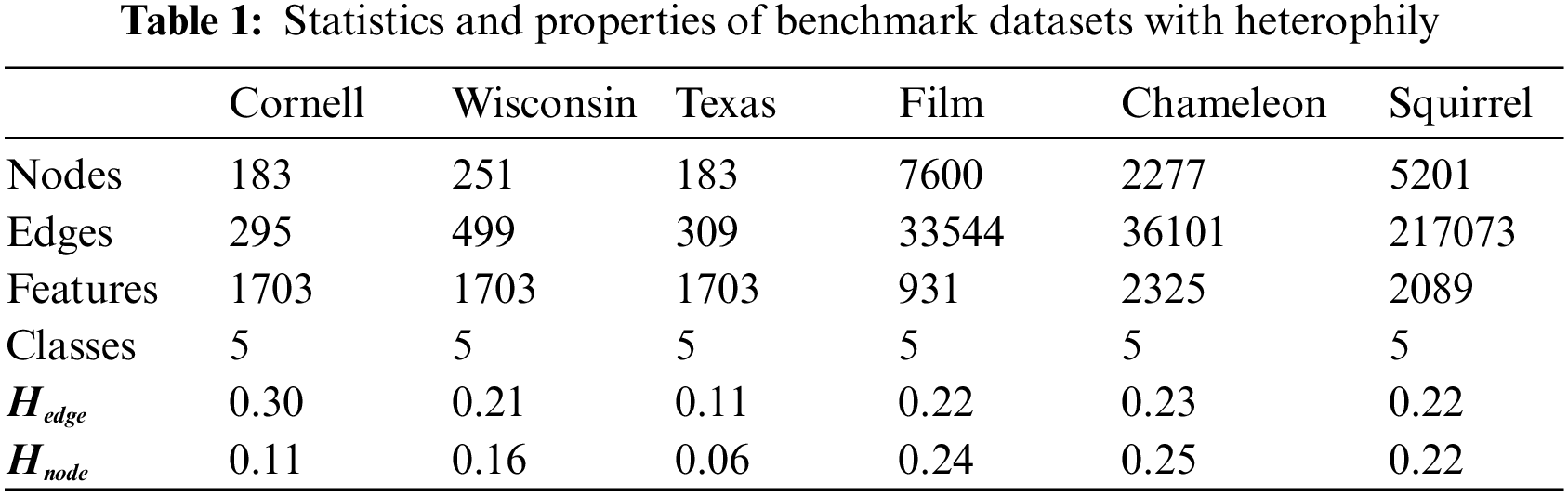
The Chameleon (Cha) and Squirrel (Squ) datasets consist of subgraphs extracted from the “Wikipedia” web pages. In these datasets, nodes represent web pages related to specific topics, while edges represent the mutual connections between these pages. Node features correspond to the information nouns found on these web pages, and the web pages are classified into 5 classes based on their monthly visitation rates.

The Film dataset is a subgraph extracted from the movie-director-actor-author relationship network. Where each node corresponds to an actor, the edge between two nodes represents both appearing on the same Wikipedia page at the same time, and the node features represent keywords on the Wikipedia page, and all the nodes are classified into 5 classes based on the type of participant.

Cornell (Cor), Texas (Tex) and Wisconsin (Wis): the above datasets are three subsets of the WebKB dataset collected at CMU, which represent links between the corresponding university web pages. In these networks, nodes represent web pages, edges are hyperlinks between them, and node features are bag-of-words representations of web pages, while all the nodes mentioned above are classified into five classes: students, programs, courses, staff, and faculty.

5.2 Baselines

In this paper, we refer to the framework outlined by Zheng et al. [5]. For heterophilic graph neural networks and select a set of representative models from various classes as the baseline networks, which are classified as follows:

Firstly, the concept of “Non-local Neighbor Extension” refers to the approach of high-order neighbor mixing or potential neighbor discovery to identify same-class nodes in the heterophilic graph that may not be directly connected to the central node but share high structural similarity. This helps introduce high homophilic information to the central node, thereby improving the quality of node representations. The core idea of the distal node spatial embedding module in SFA-HGNN is similar to this concept. To assess the practical effectiveness of this module, we have selected the following baseline models for comparative analysis:

MixHop [18] and H2GCN [19] are representatives of high-order neighbor mixing, which accomplish node embedding by aggregating the information of neighboring nodes within multiple hops from the central node.

Geom-GCN [20], GPNN [23], and Node2Seq [22] are representatives of potential neighbor discovery. They define the similarity between distant nodes and the central node based on geometric relationships in latent space, attention scores from pointer networks, or sequence orders based on attention scores. These methods prioritize the fusion and embedding of highly similar nodes.

Secondly, Graph Neural Network Architecture Refinement is to optimize the traditional GNN message aggregation and updating mechanism in order to obtain a more distinguishable node representation. Its common methods include Adaptive message aggregation, Ego-neighbor separation, and Inter-layer combination. The enhanced model's Adaptive message aggregation mechanism aligns with the proximal embedding module in this paper. We select the following baseline models to compare and analyze the practical effectiveness of this module.

FAGCN [24] and WRGNN [26] are representatives of Adaptive Message Aggregation, in which FAGCN defines high-pass and low-pass filters from the frequency domain perspective and learns the fusion ratio of the above filtering results; WRGNN models the relational edges of the heterophilic graph transformations from the spatial domain perspective, and aggregates the nodes with more significant link weights.

JK-Net [28] is a representative of inter-layer combination, which takes the embeddings from the successive layers as input for final information fusion, enabling adaptive fusion learning across different neighborhood orders.

Thirdly, in this paper, we select frequency-domain and spatial-domain graph neural networks based on the homophily assumption to compare the effectiveness of our proposed model in heterophilic graphs. The specific models are as follows:

GCN [3] and SGC [34] are frequency-domain graph neural networks, while GAT [35] and GraphSage [4] are spatial-domain graph neural networks.

Fourthly, MLP is a feedforward neural network based on node attributes, aiming to contrast the actual effects of homophily assumptions and message-passing mechanisms in heterophilic graphs [36].

5.3 Experimental Settings

Basic Parameter Settings: For training SFA-HGNN, we set the number of epochs to 500 and employ an early stopping strategy with a threshold of 200 epochs. The model parameters are adjusted based on the cross-entropy loss and accuracy of the validation set, and Adam is selected as the optimizer. The hyperparameters set for the above datasets are as follows: the hidden layer dimensions are chosen from {16, 32, 64}, learning rates are selected from {0.01, 0.005, 0.001}, dropout rates for each layer are set to {0.4, 0.5, 0.6}, and weight decay values are specified as {5E−4, 1E−4, 5E−5}. Additionally, the dataset is split into training, validation, and test sets using a ratio of 60%/20%/20%.

Key Parameter Settings: For training SFA-HGNN, we adjust the number of layers in the proximal node frequency domain embedding module to define the proximal node threshold, denoted as K∈{2,3}; sets the distal node threshold as η∈{2,3}; specifies the effective information propagation radius as ε∈{3,4,5}; sets the adaptive filter coefficient as β∈{0.3,0.4,0.5}; and defines the sample account as Sample_Account∈{2%,4%,5%,10%,20%}. The detailed rationale for these hyperparameter choices can be found in Section 5.6 of this paper.

The remaining baseline models were configured according to the parameter settings used by these papers [20,23,25,26], and others in the same experimental environment. The average predictive results were demonstrated on the test sets obtained from 10 random splits of each dataset. To ensure a fair comparison, the experimental procedures and settings were consistent with the implementation approach used by Pei et al. [20] and others. For all datasets, uniform initial feature vectors and labels were employed in the experiments.

The software environments used for the experiments in this paper are Pytorch, Pytorch Geometric, and Python 3.8. The hardware environments used are GPU RTX 3090 (2 GB); CPU Intel(R) Xeon(R) Gold 6330 @ 2.00 GHz; and RAM 80 GB.

5.4 Experiment Result

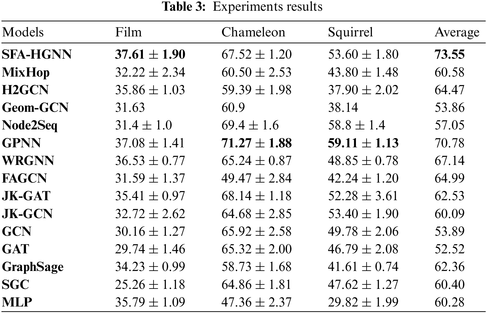
The experimental results of the model on the above six datasets are shown in Table 2, and this paper demonstrates the average accuracy and standard deviation under 10 different sets of randomized data splits.

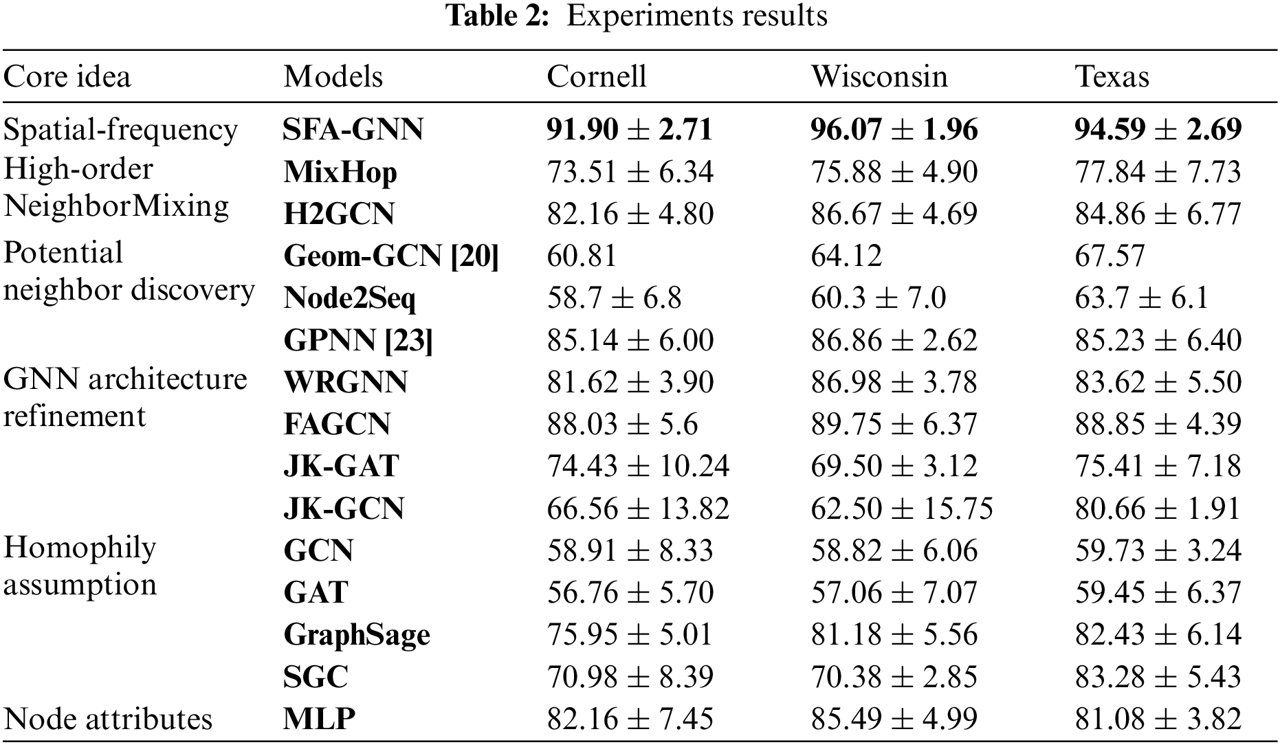
As shown in Tables 2 and 3, the optimal experimental results for each dataset are shown in bold, and the experimental results are analyzed as follows:

SFA-HGNN integrates the core ideas of Adaptive Message Aggregation and Potential Neighbor Discovery, and designs adaptive filter and oriented frequency domain attention mechanism to introduce frequency domain adaptivity for Heterophilic message passing; At the same time, we design structural coding and distal homophilic subgraph sampling to embed the rich structural information represented by random wandering migration probability for the nodes, and use it as a guide to mine the distal high homophilic nodes as a supplement to the embedding, so as to obtain the node embedding results with both spatial-frequency domain adaptivity. And the model mitigates the effects of noise and over-smoothing introduced by the High-order Neighbor Mixing model's unfiltered aggregation of distal nodes; compared with the Potential Neighbor Discovery model, it fully combines the structural role information of nodes, and avoids the problem of separating the classification of nodes from the topology of the graph.

According to the experimental results, SFA-HGNN achieves SOTA results in Cor\Wis\Tex\Film; compared with the GCN with Homophily Assumption, it has an average performance enhancement of 19.66%, which proves the validity of the motivation of the design of this model;

Compared with the GNN Architecture Refinement, the advantage of this model is that it complements the homophily information of the distal nodes and filters out the effective information of the proximal nodes by combining with the frequency domain adaptivity. As a result. As a result, the model has an average performance improvement of 6.41% and 8.56% compared to WRGNN and FAGCN based on spatial or frequency domain methods alone;

Comparing with Potential Neighbor Discovery, the advantage of this model is that it closely combines the process of potential neighbor discovery with structural information and supplements the node embedding with the learning results of the frequency domain adaptivity of the proximal nodes, which results in 2.77% and 16.5% improvement compared with the models based on the sequential ordering only, GPNN and Node2seq.

Compared with High-order Neighbor Mixing, the advantage of this model lies in the targeted acquisition of distal nodes with high homophily through structural similarity, which reduces the risk of introducing heterophilic information noise and over-smoothing, and the frequency-domain adaptive method to aggregate the proximal neighborhood’s effective information. As a result, the experimental effect is improved by 12.97% and 9.08% compared with the methods of MixHop and H2GCN that directly aggregate the nodes of each order.

Meanwhile, GPNN achieves excellent experimental results in the Chameleon and Squirrel datasets because the Hnode of the two datasets are 0.25 and 0.22, respectively, compared with the rest of the datasets, they have slightly higher homophily and relatively dense edges;

GPNN samples the initial neighborhood nodes and generates the initial node sequences through the BFS algorithm, and then carries out further learning on the node sequences, so the mechanism will tend to learn the proximal node sequences in dense graphs, and the above two datasets can provide relatively rich proximal isomorphism information and dense edges for GPNN to train the pointer network, thus achieving better experimental results in the above datasets.

To demonstrate the effectiveness of the node embedding and classification in this study, we performed t-SNE visualization analysis on the node embedding results of the Wisconsin and Texas datasets after 100 training epochs. The following figure, Fig. 6, illustrates this analysis:

Figure 6: T-SNE results

As shown in the Fig. 6, the SFA-HGNN model achieves distinct separation between different classes of nodes with a significant inter-class distance and a compact intra-class distance after just 100 training epochs. This layout formation indicates that SFA-HGNN effectively discriminates between different classes.

5.5 Parameter Sensitivity Analysis

5.5.1 Selection of Network Prior Information and Hyperparameter Range

This section sets the core hyperparameter value range in combination with prior information, defined as follows:

Effective information transmission radius ε: Considering the network diameter reflects the longest distance between two nodes within the connected components, it is hard to represent the main transmission path in the message transmission process. Therefore, this paper uses the average value of the network Radius and the average shortest path length Asp as the basis for selecting ε. This can reflect the actual path length of message transmission among many nodes and ensure that the sampled subgraph contains ample information from distant nodes. The specific definition is as follows:

ε∈[Radius+Asp2−1,Radius+Asp2+1](41)

Distal node threshold η and proximal node threshold K: The number of each-order neighboring nodes originating from the central node is defined as HopNum. Then, the similarity of attribute vectors between these nodes and the central node is Fsimilarity, along with the count of homophilic nodes HomoNum and the proportion of homophilic nodes HomoAccount. Based on the trends of these indicators with the change in the sampling order, they are used as the basis for selecting the above-mentioned hyperparameters. The relevant definitions are as follows:

HopNumr=Nr(nodeseeds)={v:d(u,v)=r,u∈nodeseeds}(42)

Fsimilarityr=1VNr∑u∈nodeseeds,v∈Nr(u)xu⋅xv|xu||xv|(43)

HomoNumr={v:labelv=labelu,u∈nodeseeds,v∈Nr(u)}(44)

HomoAccountr=HomoNumrNumNodesr(45)

Distal node sampling ratio (Sample_Account): To achieve a relatively balanced information density for both near and distal message transmission, the distal node sampling ratio is set. Ensuring a dynamic balance between the number of nodes on the near and far sides while maintaining the quality of homophilic information. The specific definition is as follows:

Nnear(nodeseeds)≈Nfar(nodeseeds)(46)

Sample_Account=Nfar(nodeseeds)∑r=ηε⁡HopNumr(47)

In summary, the relevant experiments are carried out by taking the validation set nodes defined in the previous section, and the results of the above a priori information calculations are shown below:

As shown in Fig. 7 and combined with Eq. (41), this study defines the preliminary range for ε as ε∈{3,4,5,6}, ensuring that ε is slightly larger than Asp to ensure sufficient sampling of far-end effectiveness information.

Figure 7: Dataset prior information

As shown in Fig. 7, the fluctuations in “HomoNum” for various datasets with respect to the order are quite noticeable. For the Wis/Tex/Cor dataset, the number of homophilic nodes reaches its peak at the 2nd order, followed by a decreasing trend. The Film/Squ/Cha dataset exhibits an initial increase followed by a decrease, with the peaks mainly concentrated at the 3rd and 4th orders. Notably, Cha is relatively more stable compared to other datasets. Given that the aforementioned datasets fall into five categories, this paper sets 20% as the threshold for determining the strength of effective information at each order.

As shown in Fig. 7, the fluctuations in “HomoAccount” for the Wis/Tex/Cor dataset are more pronounced, but strong overall homophilic information across different orders. For the Film/Squ/Cha dataset, “HomoAccount” remains relatively stable, with a general fluctuation around 20%.

The overarching principle for setting the range of “K” and “η” is as follows: Using the proximal node threshold “K” to define the proximal neighborhood range with the relatively higher “HomoAccount” and more significant homophilic node count (“HomoNum”) to mitigate noise interference from neighboring node message propagation.

Similarly, using the distal node threshold “η” to define the far-end node range with a lower “HomoAccount” and a relatively smaller “HomoNum”, thereby constructing a far-end homophilic subgraph to enhance the quality of information aggregation. In summary, this paper tentatively selects K∈{1,2,3} and η∈{2,3,4}.

As shown in Fig. 7, nodes from Wis/Tex/Cor/Squ are primarily concentrated at the 3rd order, while nodes from the Film/Squ dataset are predominantly found at the 4th order. Considering the definitions of HopNum, “K” and “η”, this study tentatively sets the distal node sampling ratio Sample_Account∈{1%,1.5%,2%,4%,5%,10%,20%,25%} to ensure a relative balance in information density between the near and far ends.

5.5.2 Parameter Experimental Analysis

This section aims to integrate the aforementioned prior information with the intrinsic characteristics of the dataset. We design four sets of hyperparameters for each dataset, adjusting the information density of proximal and distal node connections. These sets are specifically tailored to embed information for nodes at close, intermediate, middle-distance, and far distances. The specific parameter designs are shown in Tables 4 and 5.

The effective information propagation radius ε, and the threshold for distal nodes η, are employed to constrain the upper and lower bounds of distal nodes. And sample a specific proportion of nodes by Sample_Account. Hence, when η is broader and Sample_Account is higher, the model tends to incorporate information from distal nodes into the central node embedding via spatial domain methods.

Conversely, the proximal node threshold K, serves as an upper limit for proximal nodes. A larger value of K implies a broader coverage of proximal node information, leading the model to favor embedding proximal node information into the central node via frequency domain methods.

Based on the aforementioned combination of parameters, the experimental results are shown in Fig. 8a. Additionally, employing the aforementioned optimal parameters, sensitivity analysis is conducted on the adaptive filter coefficient β across various datasets, as shown in Fig. 8b:

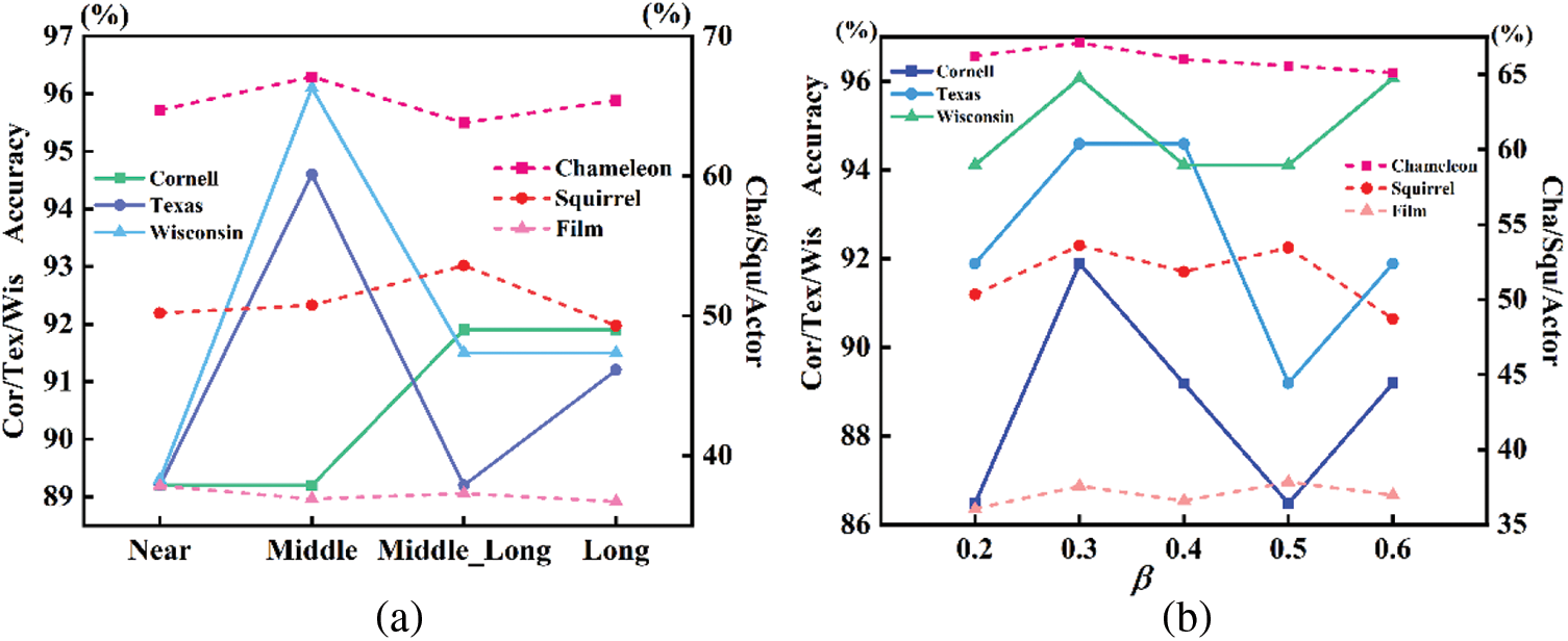
Figure 8: Sensitivity analysis

As shown in Fig. 8, the optimal hyperparameters for the aforementioned datasets predominantly cluster around the mid-distance range. This suggests that embedding a balanced combination of proximal neighborhood information and distal homophily information can lead to superior representation. Specifically, the Cor/Tex/Wis datasets are particularly sensitive to changes in the primary information embedding method. Overemphasizing either proximal or distal information can result in a decline in model performance. Conversely, the experimental results for the Film dataset are relatively stable, showing low sensitivity to changes in the embedding of proximal or distal information. The Cha/Squ datasets obtain their optimal results around mid-distance embedding parameters, with the Squirrel dataset showing a preference for spatial domain methods to aggregate distal node information for optimal node representation.

As shown in Fig. 8, compared to other datasets, Cor/Wis/Tex exhibit higher sensitivity to variations in the adaptive filter coefficient β. Optimal results across datasets converge around β = 0.3, proving the notion that moderate scaling of the convolution kernel across different frequency bands is conducive to learning the best embedding representation. If β is excessively big, it may diminish the learning capability for certain frequency bands, leading to information loss.

5.6 Ablation Experiment

5.6.1 Frequency Domain Embedding Module Ablation Analysis

The aim of this section is to adapt the information fusion method in the message aggregation process by modifying Eq. (37) as follows to verify the effectiveness of frequency domain adaptivity for learning proximal nodes:

hi(l)=βhi(0)+∑j∈NiwijAblationdidjhj(l−1)∈RF×1(48)

wij1=tanh⁡(MLP2F→1([hi||hj]))(49)

wij2=Sigmoid(MLP2F→1([hi||hj]))(50)

wij3=Relu(MLP2F→1([hi||hj]))(51)

As described above, a linear transformation is applied to the concatenated vectors of dimension 2F using a feedforward neural network MLP to obtain an information fusion scalar. The weight coefficient wij1 is defined to eliminate the “frequency domain orientation information prior”. Additionally, wij2 and wij3 are introduced, incorporating two nonlinear activation functions to fix the edge weight coefficients positively during the message-passing process, thereby canceling the frequency domain adaptivity.

For the experiments conducted on the aforementioned datasets, the optimal parameter set defined in Section 5.6.1 is employed. The data is randomly partitioned and the experiment is repeated 10 times to obtain results, presenting the average values across all datasets. Other settings remain consistent with Section 4.3. The experimental outcomes are shown in Fig. 9.

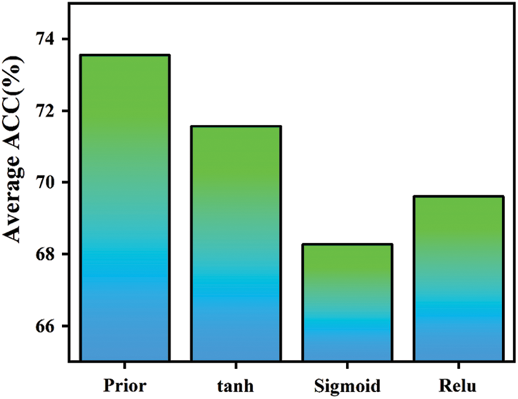
Figure 9: Frequency domain module ablation results

As shown in Fig. 9, the introduction of the frequency domain orientation information prior incorporates the similarity between the attribute vectors of the central node and its distant neighborhood. This reflection captures the central node's preferences for proximal and distal information. Based on the magnitude of these preference indicators, the embedding process selectively learns high-frequency and low-frequency signals from the proximal neighborhood. As a result, an average of 73.55% optimal experimental outcomes is achieved across all datasets. Compared to the sole utilization of the nonlinear activation function tanh to achieve frequency domain adaptivity in wij1, there is a notable experimental enhancement of 2.0%.

On the other hand, wij2 and wij3 map the information fusion weights to positive values, effectively making the message-passing process equivalent to a weighted averaging of neighborhood information. This could introduce the influence of proximal noise during the heterophilic graph neighborhood aggregation process. Consequently, when compared to the experimental results obtained by introducing prior, wij2 and wij3 exhibit reduced performance by 5.2% and 4.0%, respectively.

5.6.2 Spatial Embedding Module Ablation Analysis

To validate the effectiveness of the spatial domain embedding module in capturing distal node homophily information, a comparison is conducted among three sets of neighboring nodes: first-order neighborhood nodes, the top 5 neighborhood nodes sampled based on attention scores from the Node2Seq model, and distal nodes selected using random walk transition probabilities. The relative homophily measure, Hnode, with respect to the central node is computed for these sets. Utilizing the optimal hyperparameters designed in Section 5.6.2, a distal homophily subgraph is constructed for all nodes in each dataset. Within this subgraph, the distal nodes associated with the central node via virtual high-speed links are used to calculate Hnode.

Moreover, Zhu et al. [19] theoretically established that second-order neighbor homophily information dominates in heterophilic network nodes. Therefore, this study adopts the second-order neighbor attribute vector similarity, Fsimilaritytwohop, as a baseline. Additionally, the attribute vector similarity, Fsimilarityfar, between the central node and distal nodes is calculated. By comparing these two measures, the model's preferred nodes are validated to possess not only homophily but also attribute vector similarity. The results of the two aforementioned experiments are presented in Fig. 10.

Figure 10: Spatial domain module ablation results

As depicted in Fig. 10, this study utilizes a node selection mechanism guided by random walks to model node structural similarity through transition probabilities. This mechanism filters out distal homophilic nodes distributed across the heterophilic graph. This approach, compared to node selection based on attention scores, effectively leverages the inherent topological information of the graph, leading to enhanced node selection results. Consequently, compared to 1-Hop Neighbors and Rank with Attention, the average improvement is 22% and 9.6%, respectively.

Based on the earlier discussion, second-order neighbors predominantly exhibit central node homophily information. Therefore, it serves as the baseline for highlight the relationship between the feature vectors of the selected distal nodes and the central node. As shown in Fig. 10b, across all datasets, the distal nodes exhibit an improvement over second-order neighbor similarity, with an average improvement of 0.102. This experiment validates that the random walk transition probabilities originating from the central node effectively capture the varying strengths of both node homophily and attribute vector similarity between nodes.

Simultaneously, adhering to the optimal parameter settings defined in Section 5.6.1, in the Wis, Cor, and Tex datasets, the Sample_Account is set to {2%,4%,5%,10%,20%}. And compute the distal node homophilyfar and distal neighborhood Fsimilarityfar, for various Sample_Account. This process aims to verify the relationship between higher-order random walk transition probabilities and the similarity and homophily information of sampled nodes, as shown in Fig. 11.

Figure 11: Results of correlation verification

As mentioned earlier, Sample_Account is defined as the sampling ratio based on the priority of node high-order random walk transition probability scores. As this value increases, the structural similarity between the sampled distant nodes and the central node decreases. As shown in the figure above, both Homophilyfar and Fsimilarityfar decrease as Sample_Account increases, and their overall trends are similar. This experimental result further confirms the hypothesis of our paper: a sampling mechanism guided by higher-order random walk transition probabilities tends to prioritize the selection of distal nodes with high attribute vector similarity and a significant homophily. Additionally, there appears to be a positive correlation between node homophily, attribute vector similarity, and the score of higher-order random walk transition probabilities (i.e., node structural similarity S).

6  Conclusion and Future Work

This paper introduces the SFA-HGNN model to address the challenges that traditional GNNs face when applied to heterophilic graphs, specifically the issues of “missing modeling of distal nodes” and “failure of homophily assumption”. To tackle the former, SFA-HGNN employs a “distal spatial embedding module” based on higher-order random walk transition probabilities to sample and aggregate information from distal nodes with high structural similarity, thereby enhancing the model’s ability to capture distal node characteristics. To address the latter, the “proximal frequency domain embedding module” is designed to adaptively learn high and low-frequency signals from proximal nodes to fuse valuable information, reducing noise interference introduced by the failure of the homophily assumption on the low-pass filters.

The paper concludes by demonstrating the excellent performance of SFA-HGNN in heterophilic network node classification tasks, explaining the theoretical mechanisms behind hyperparameter selection and the effectiveness of each module. The positive correlation among node attribute vector similarity, node homophily, and node structural similarity is validated through experiments. However, the model still has room for improvement. For instance, the structural encoding process essentially is pre-embedding node information, and its time complexity is closely related to the complexity of network nodes and edges. Future work could focus on further improving the model in response to this challenge.

Acknowledgement: We are grateful to the editors and reviewers for their helpful suggestions, which have greatly improved this paper.

Funding Statement: This work is supported by the Fundamental Research Funds for the Central Universities (Grant No. 2022JKF02039).

Author Contributions: The authors confirm contribution to the paper as follows: study conception and design: Lanze Zhang, Yijun Gu; data collection: Lanze Zhang, Jingjie Peng; analysis and interpretation of results: Lanze Zhang, Jingjie Peng; draft manuscript preparation: Lanze Zhang, Jingjie Peng. All authors reviewed the results and approved the final version of the manuscript.

Availability of Data and Materials: If the SFA-HGNN model and relevant experimental data are needed, readers are advised to contact the author, and the author will provide you with help in the first place.

Conflicts of Interest: The authors declare that they have no conflicts of interest to report regarding the present study.

References

1. Zhou, J., Cui, G., Hu, S., Zhang, Z., Yang, C. et al. (2020). Graph neural networks: A review of methods and applications. AI Open, 1, 57–81. https://doi.org/10.1016/j.aiopen.2021.01.001 [Google Scholar] [CrossRef]

2. Zeng, H., Zhou, H., Srivastava, A., Kannan, R., Prasanna, V. (2019). Graphsaint: Graph sampling based inductive learning method. https://doi.org/10.48550/arXiv.1907.04931 [Google Scholar] [CrossRef]

3. Kipf, T. N., Welling, M. (2016). Semi-supervised classification with graph convolutional networks. https://doi.org/10.48550/arXiv.1609.02907 [Google Scholar] [CrossRef]

4. Hamilton, W., Ying, Z., Leskovec, J. (2017). Inductive representation learning on large graphs. In: Advances in neural information processing systems 30. Long Beach, CA, USA. [Google Scholar]

5. Zheng, X., Liu, Y., Pan, S., Zhang, M., Jin, D. et al. (2022). Graph neural networks for graphs with heterophily: A survey. https://doi.org/10.48550/arXiv.2202.07082 [Google Scholar] [CrossRef]

6. Nt, H., Maehara, T. (2019). Revisiting graph neural networks: All we have is low-pass filters. https://doi.org/10.48550/arXiv.1905.09550 [Google Scholar] [CrossRef]

7. Yan, Y., Hashemi, M., Swersky, K., Yang, Y., Koutra, D. (2022). Two sides of the same coin: Heterophily and oversmoothing in graph convolutional neural networks. 2022 IEEE International Conference on Data Mining (ICDM), pp. 1287–1292. Orlando, FL, USA. https://doi.org/10.1109/ICDM54844.2022.00169 [Google Scholar] [CrossRef]

8. Mostafa, H., Nassar, M., Majumdar, S. (2021). On local aggregation in heterophilic graphs. https://doi.org/10.48550/arXiv.2106.03213 [Google Scholar] [CrossRef]

9. Zheng, X., Zhang, M., Chen, C., Zhang, Q., Zhou, C. et al. (2023). Auto-heg: Automated graph neural network on heterophilic graphs. https://doi.org/10.48550/arXiv.2302.12357 [Google Scholar] [CrossRef]

10. Song, Y., Zhou, C., Wang, X., Lin, Z. (2023). Ordered GNN: Ordering message passing to deal with heterophily and over-smoothing. https://doi.org/10.48550/arXiv.2302.01524 [Google Scholar] [CrossRef]

11. Qiao, Z., Luo, X., Xiao, M., Dong, H., Zhou, Y. et al. (2023). Semi-supervised domain adaptation in graph transfer learning. https://doi.org/10.48550/arXiv.2309.10773 [Google Scholar] [CrossRef]

12. Hu, Z., Dong, Y., Wang, K., Sun, Y. (2020). Heterogeneous graph transformer. Proceedings of the Web Conference 2020, pp. 2704–2710. Taipei, Taiwan. https://doi.org/10.1145/3366423.3380027 [Google Scholar] [CrossRef]

13. Zhao, J., Wang, X., Shi, C., Hu, B., Song, G. et al. (2021). Heterogeneous graph structure learning for graph neural networks. Proceedings of the AAAI Conference on Artificial Intelligence, 35(5), 4697–4705. https://doi.org/10.1609/aaai.v35i5.16600 [Google Scholar] [CrossRef]

14. Wang, X., Ji, H., Shi, C., Wang, B., Ye, Y. et al. (2019). Heterogeneous graph attention network. The World Wide Web Conference, pp. 2022–2032. San Francisco, CA, USA. https://doi.org/10.1145/3308558.3313562 [Google Scholar] [CrossRef]

15. Gilmer, J., Schoenholz, S. S., Riley, P. F., Vinyals, O., Dahl, G. E. et al. (2017). Neural message passing for quantum chemistry. International Conference on Machine Learning (PMLR), pp. 1263–1272. Sydney, Australia. [Google Scholar]

16. Wang, Y., Derr, T. (2021). Tree decomposed graph neural network. Proceedings of the 30th ACM International Conference on Information Knowledge Management, pp. 2040–2049. The University of Queensland. https://doi.org/10.1145/3459637.3482487 [Google Scholar] [CrossRef]

17. Jin, W., Derr, T., Wang, Y., Ma, Y., Liu, Z. et al. (2021). Node similarity preserving graph convolutional networks. Proceedings of the 14th ACM International Conference on Web Search and Data Mining, pp. 148–156. https://doi.org/10.1145/3437963.3441735 [Google Scholar] [CrossRef]

18. Abu-El-Haija, S., Perozzi, B., Kapoor, A., Alipourfard, N., Lerman, K. et al. (2019). Mixhop: Higher-order graph convolutional architectures via sparsified neighborhood mixing. International Conference on Machine Learning (PMLR), pp. 21–29. Long Beach, CA, USA. [Google Scholar]

19. Zhu, J., Yan, Y., Zhao, L., Heimann, M., Akoglu, L. et al. (2020). Beyond homophily in graph neural networks: Current limitations and effective designs. Advances in Neural Information Processing Systems, 33, 7793–7804. [Google Scholar]

20. Pei, H., Wei, B., Chang, K. C. C., Lei, Y., Yang, B. (2020). Geom-GCN: Geometric graph convolutional networks. https://doi.org/10.48550/arXiv.2002.05287 [Google Scholar] [CrossRef]

21. Liu, M., Wang, Z., Ji, S. (2021). Non-local graph neural networks. IEEE Transactions on Pattern Analysis and Machine Intelligence, 44(12), 10270–10276. https://doi.org/10.1109/TPAMI.2021.3134200 [Google Scholar] [PubMed] [CrossRef]

22. Yuan, H., Ji, S. (2021). Node2seq: Towards trainable convolutions in graph neural networks. https://doi.org/10.48550/arXiv.2101.01849 [Google Scholar] [CrossRef]

23. Yang, T., Wang, Y., Yue, Z., Yang, Y., Tong, Y. et al. (2022). Graph pointer neural networks. Proceedings of the AAAI Conference on Artificial Intelligence, 36(8), 8832–8839. https://doi.org/10.1609/aaai.v36i8.20864 [Google Scholar] [CrossRef]

24. Bo, D., Wang, X., Shi, C., Shen, H. (2021). Beyond low-frequency information in graph convolutional networks. Proceedings of the AAAI Conference on Artificial Intelligence, 35(5), 3950–3957. https://doi.org/10.1609/aaai.v35i5.16514 [Google Scholar] [CrossRef]

25. Luan, S., Hua, C., Lu, Q., Zhu, J., Zhao, M. et al. (2021). Is heterophily a real nightmare for graph neural networks to do node classification? https://doi.org/10.48550/arXiv.2109.05641 [Google Scholar] [CrossRef]

26. Suresh, S., Budde, V., Neville, J., Li, P., Ma, J. et al. (2021). Breaking the limit of graph neural networks by improving the assortativity of graphs with local mixing patterns. Proceedings of the 27th ACM SIGKDD Conference on Knowledge Discovery Data Mining, pp. 1541–1551. https://doi.org/10.1145/3447548.3467373 [Google Scholar] [CrossRef]

27. Jin, D., Yu, Z., Huo, C., Wang, R., Wang, X. et al. (2021). Universal graph convolutional networks. In: Advances in neural information processing systems 34, pp. 10654–10664. [Google Scholar]

28. Xu, K., Li, C., Tian, Y., Sonobe, T., Kawarabayashi, K. I. et al. (2018). Representation learning on graphs with jumping knowledge networks. International conference on machine learning (PMLR), pp. 5453–5462. Stockholm, Sweden. [Google Scholar]

29. Chen, M., Wei, Z., Huang, Z., Ding, B., Li, Y. (2020). Simple and deep graph convolutional networks. International Conference on Machine Learning (PMLR), pp. 1725–1735. Cancun, Mexico. [Google Scholar]

30. Kong, L., Chen, Y., Zhang, M. (2022). Geodesic graph neural network for efficient graph representation learning. In: Advances in neural information processing systems 35, pp. 5896–5909. [Google Scholar]

31. Li, P., Wang, Y., Wang, H., Leskovec, J. (2020). Distance encoding: Design provably more powerful neural networks for graph representation learning. In: Advances in neural information processing systems 33, pp. 4465–4478. [Google Scholar]

32. Shervashidze, N., Schweitzer, P., van Leeuwen, E. J., Mehlhorn, K., Borgwardt, K. M. (2011). Weisfeiler-lehman graph kernels. Journal of Machine Learning Research, 12(9), 2539–2561. [Google Scholar]

33. Dai, E., Jin, W., Liu, H., Wang, S. (2022). Towards robust graph neural networks for noisy graphs with sparse labels. Proceedings of the Fifteenth ACM International Conference on Web Search and Data Mining, pp. 181–191. Electr Network. [Google Scholar]

34. Wu, F., Souza, A., Zhang, T., Fifty, C., Yu, T. et al. (2019). Simplifying graph convolutional networks. International Conference on Machine Learning (PMLR), pp. 6861–6871. Long Beach, CA, USA. [Google Scholar]

35. Velickovic, P., Cucurull, G., Casanova, A., Romero, A., Lio, P. et al. (2017). Graph attention networks. Statistics. https://doi.org/10.48550/arXiv.1710.10903 [Google Scholar] [CrossRef]

36. Zaknich, A. (1998). Introduction to the modified probabilistic neural network for general signal processing applications. IEEE Transactions on Signal Processing, 46(7), 1980–1990. https://doi.org/10.1109/78.700969 [Google Scholar] [CrossRef]