Optimizing UCS Prediction Models through XAI-Based Feature Selection in Soil Stabilization

1  Introduction

The unconfined compressive strength (UCS) is a major mechanical characteristic of soil. The determination of the safe load capacity and stability of soils is the main usage of UCS [1], it accommodates the specifications of the design along with the performance evaluation of geotechnical structures such as pavements, embankments, retaining walls, and shallow foundations.

UCS testing is a major source of information on the improvement process of soil stabilization techniques when stabilization by chemical means is involved. Typically, the methods consist in adding lime, cement, fly ash, or another industrial by-product [1]. These binders change the microstructure and the minerals of the soil and these changes contribute to the strengthening and the durability of soil through both pozzolanic and cementitious reactions [2,3].

Even though laboratory UCS testing is dependable, it is a very time-consuming process, and it requires a lot of work, sample preparation and curing, which are usually the reasons for project delays. This situation has led to the growing interest in data-driven methods, especially machine learning (ML). The ML techniques can acknowledge the complex relationships that occur between geotechnical, compaction, and chemical parameters and hence can provide rapid and cost-effective methods that can be used instead of experimental testing [4,5].

Applications of ML algorithms in geotechnical engineering have been shown immense potential in the prediction of swelling potential, California Bearing Ratio, and loss of strength on immersion durability, further extending to the prediction of the unconfined compressive strength. For instance, advanced tree-based techniques, i.e., Random Forest (RF) and XGB, were applied with excellent success to predict UCS from petrographic examinations and non-destructive tests and prove to possess the capability to deal with advanced material characteristics [6]. Moreover, the ability of these algorithms to integrate different models (ensemble models) has enhanced prediction accuracy and consistency, especially in handling the intricate relationships among various geotechnical properties and how they influence soil behavior [7]. Such an ability is particularly critical in applications where soil shear strength prediction, a significant geotechnical engineering practice, is crucial for infrastructure stability [8].

Since the last decade, RF, Gradient Boosting (GB), XGB, DT, and K-Nearest Neighbors (KNN) Machine Learning algorithms were applied to UCS prediction with successful accuracy. These models can process a range of inputs such as Atterberg limits (LL, PL, PI), specific gravity, maximum dry density (MDD), optimum moisture content (OMC), stabilizer chemical composition (SiO2, CaO, Al2O3, MgO), binder dosage, and curing time. Based on big data sets, they are able to recognize hidden patterns and complex dependencies that cannot be readily recognized by empirical or regression-based models.

However, a significant drawback of most high-performing ML models is their “black-box” nature, precluding interpretability. In reality among engineers, stakeholders typically require correct predictions along with comprehensible explanations about why particular parameters control the outcome. Failure to provide such interpretability hinders complete trust in data-driven predictions alone, particularly in safety-critical applications such as geotechnics.

1.1 Explainable AI for Feature Selection

Explainable Artificial Intelligence (XAI) techniques have appeared to bridge the interpretability gap in ML. Of these, SHapley Additive exPlanations (SHAP) is a mathematically sound and model-agnostic method for quantifying feature contributions [9]. Drawing from cooperative game theory, SHAP attributes a value of importance to every feature to reflect its average marginal contribution to the prediction over all permutations of feature combinations [10].

SHAP is used in geotechnical engineering to explain ML predictions for soil compaction optimization, slope stability analysis, and strength of cemented soils prediction.

Feature selection, under the direction of strong importance measures such as SHAP values, can drastically enhance model efficiency, minimize overfitting danger, and decrease the data acquisition cost. Practically, minimizing the features of the input implies fewer laboratory tests, less sample workup, and quicker project times, without a drastic loss in accuracy.

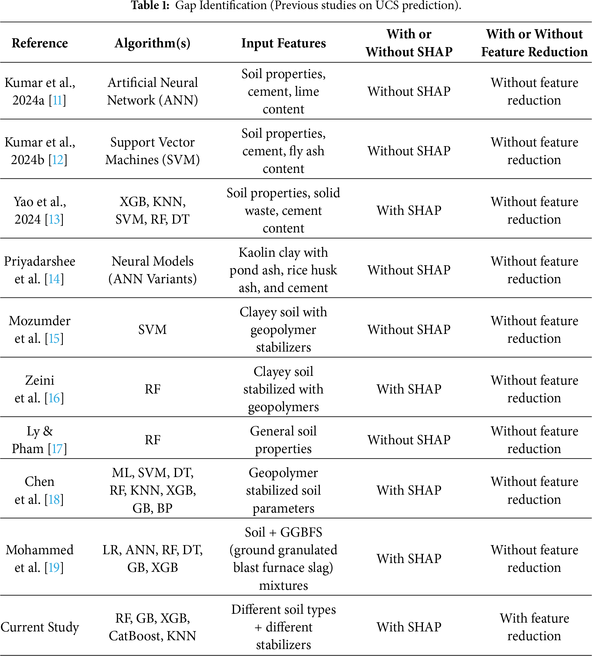
An overview of recent studies on UCS prediction using ML shows some important advancement, but also clear limits that define the research gap addressed in this work. Kumar et al. [11] applied ANN to cement-lime stabilized soils and obtained good predictive accuracy in early studies. However, these models concentrated on one algorithm alone and did not implement interpretability techniques such as SHAP, nor did they engage with diminished feature sets. Similarly, Kumar et al. [12] employed support vector machines (SVM) for cement–fly ash stabilized soils to promising effect, but again the concentration was limited, with no comparative study over multiple algorithms and no attempt at explainable or feature-reduced modeling.

Additional studies, such as Yao et al. [13], contrasted hybrid models that consisted of XGB, KNN, SVM, RF, and DT, and demonstrated that a hybrid XGB approach yielded outstanding UCS predictions for stabilized cohesive soils. Though SHAP analysis was applied, model accuracy alone was the emphasis of the study, without ascertaining whether performance with fewer input features was possible. Priyadarshee et al. [14] also showed that it is possible to model non-linear effects of pond ash, rice husk ash, and cement on kaolin soils using neural models, although their work lacked interpretability analysis and feature selection.

Other research looked at geopolymer stabilization. Mozumder et al. [15] applied SVM to geopolymer-stabilized clay with satisfactory accuracy, but the research was hampered by the absence of modern explainable AI techniques. Zeini et al. [16] applied RF to geopolymer soils and included SHAP analysis for interpretability, but the approach was restricted to a single algorithm and did not examine systematic feature removal. Similarly, Ly & Pham [17] used RF to predict UCS based on common soil properties, but their dataset was relatively small and lacked SHAP-based interpretation.

Comparative research has also been published. Chen et al. [18] compared a wide range of models like SVM, RF, KNN, XGB, GB, and backpropagation neural networks for geopolymer-stabilized soils and applied SHAP for interpretability. While their research advanced model comparison one step further, it stopped short of systematically reducing features to consider the simplicity-accuracy trade-off. More recently, Mohammed et al. [19] used explainable AI (XAI) in UCS prediction of soils mixed with ground granulated blast furnace slag (GGBS), and SHAP was employed to calculate feature importance. However, although interpretability was taken into account, the research did not conduct systematic feature reduction experiments (e.g., 12, 8, and 5 features).

Cumulatively, the literature demonstrates satisfactory progress in UCS prediction using various ML algorithms like ANN, SVM, RF, XGB, and hybrid models. A few recent studies also began incorporating SHAP for interpretability. However, there is one common research gap in all of them: there are no studies that compare multiple ML algorithms systematically in conjunction with using SHAP both for feature importance as well as guided feature reduction. Most of the research either focuses on predictive accuracy alone or uses SHAP solely for interpretation without testing on reduced-feature models. This knowledge gap calls for a holistic framework that not only predicts UCS with high accuracy but also enhances interpretability and efficiency through SHAP-based feature reduction. The gap is shown in Table 1.

1.2 Contribution of This Study

1.   This study addresses the above research gap by developing an integrated UCS prediction framework that combines multi-model ML prediction with SHAP-based interpretability and feature reduction. The main contributions are:

Multi-Model UCS Predictor Development: A dataset of 12 geotechnical and chemical parameters is used to train five machine learning algorithms (RF, GB, XGB, CatBoost, and KNN) to model UCS for various soil–stabilizer combinations.

(b)   SHAP-Based Feature Ranking and Reduction: The significance of each of the 12 features is ranked using SHAP analysis. Model-agnostic rankings are used to determine the top 8 and top 5 most influential features.

(c)   In order to evaluate the trade-offs between accuracy, interpretability, and data efficiency, models are retrained using the reduced feature sets and compared to the full-feature models using R2, RMSE, MSE, and MAE.

(d)   Engineering Understanding of Feature Importance: The alignment of statistical importance with accepted geotechnical theory is validated by interpreting the SHAP rankings in the context of soil stabilization mechanisms.

Rest of the paper roadmap. Section 2 details the materials and methods: the curated multi-source dataset and 12 input features (Section 2.1), the five machine-learning algorithms RF, GB, XGB, CatBoost, and KNN (Section 2.2), the SHAP procedure for interpretability (Section 2.3), and the comparative design testing three feature sets (12, 8, and 5) with R2, RMSE, MSE, and MAE (Section 2.4). Section 3 presents the results and discussion: data exploration (distributions, summary statistics, correlations), baseline performance with all 12 features, SHAP-based feature importance, and reduced-feature model performance, with supporting figures and tables. Section 4 provides the conclusions, practical implications for cost-efficient UCS testing, and directions for future work.

2  Materials and Methods

In this study, we designed a structured framework for predicting the unconfined compressive strength (UCS) of stabilized soils using machine learning and explainable AI techniques. The proposed methodology, illustrated in Fig. 1, begins with the collection and preprocessing of experimental data from published studies, covering 12 geotechnical and chemical parameters. This dataset, described in detail in Section 2.1, provided the basis for model training and evaluation. Five algorithms Random Forest, Gradient Boosting, Extreme Gradient Boosting, CatBoost, and K-Nearest Neighbors were then implemented under three scenarios: all 12 features, the top 8 features, and the top 5 features identified using SHAP analysis. To ensure robust evaluation, model performance was assessed with R2, RMSE, MSE, and MAE. SHAP analysis was further used to interpret feature importance, consistently highlighting CaO content, curing period, stabilizer dosage, and compaction parameters as the dominant predictors of UCS. The comparative analysis showed that boosting-based models maintained high accuracy even with fewer features, demonstrating that SHAP-guided feature reduction enables cost-effective, interpretable prediction without sacrificing performance. To operationalize this framework, the dataset preparation steps are presented in Section 2.1, followed by a description of the applied machine learning algorithms in Section 2.2.

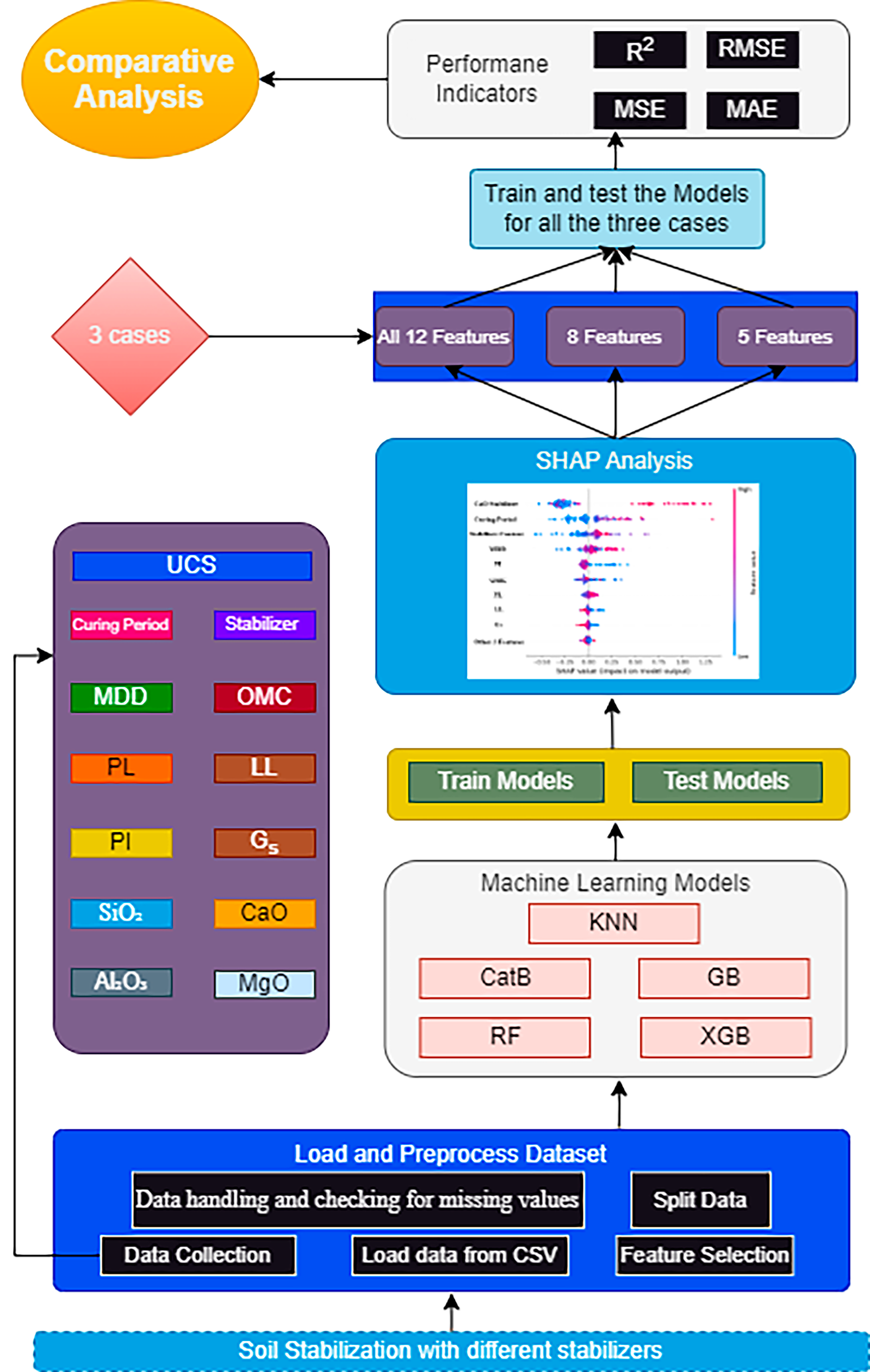
Figure 1: Proposed methodology.

2.1 Dataset and Preprocessing

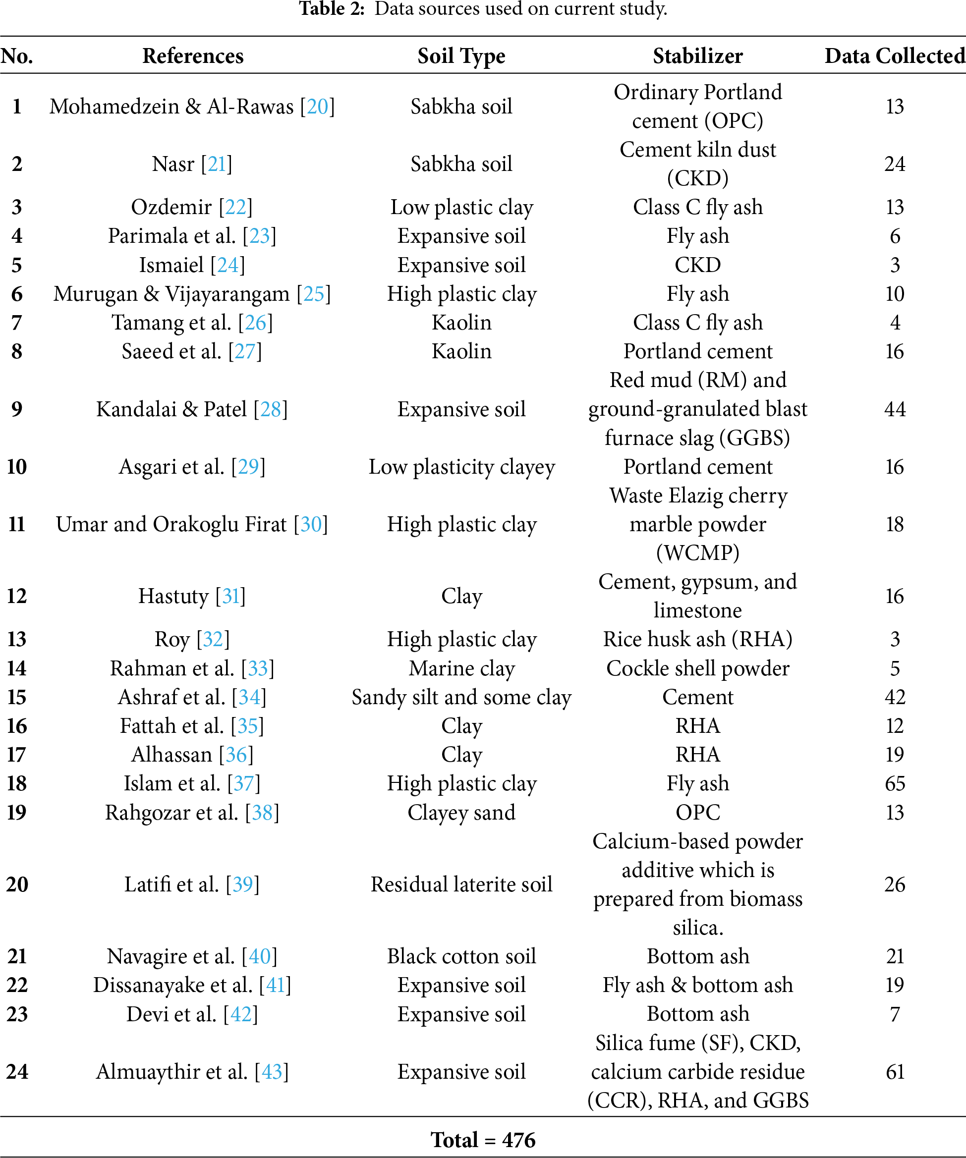
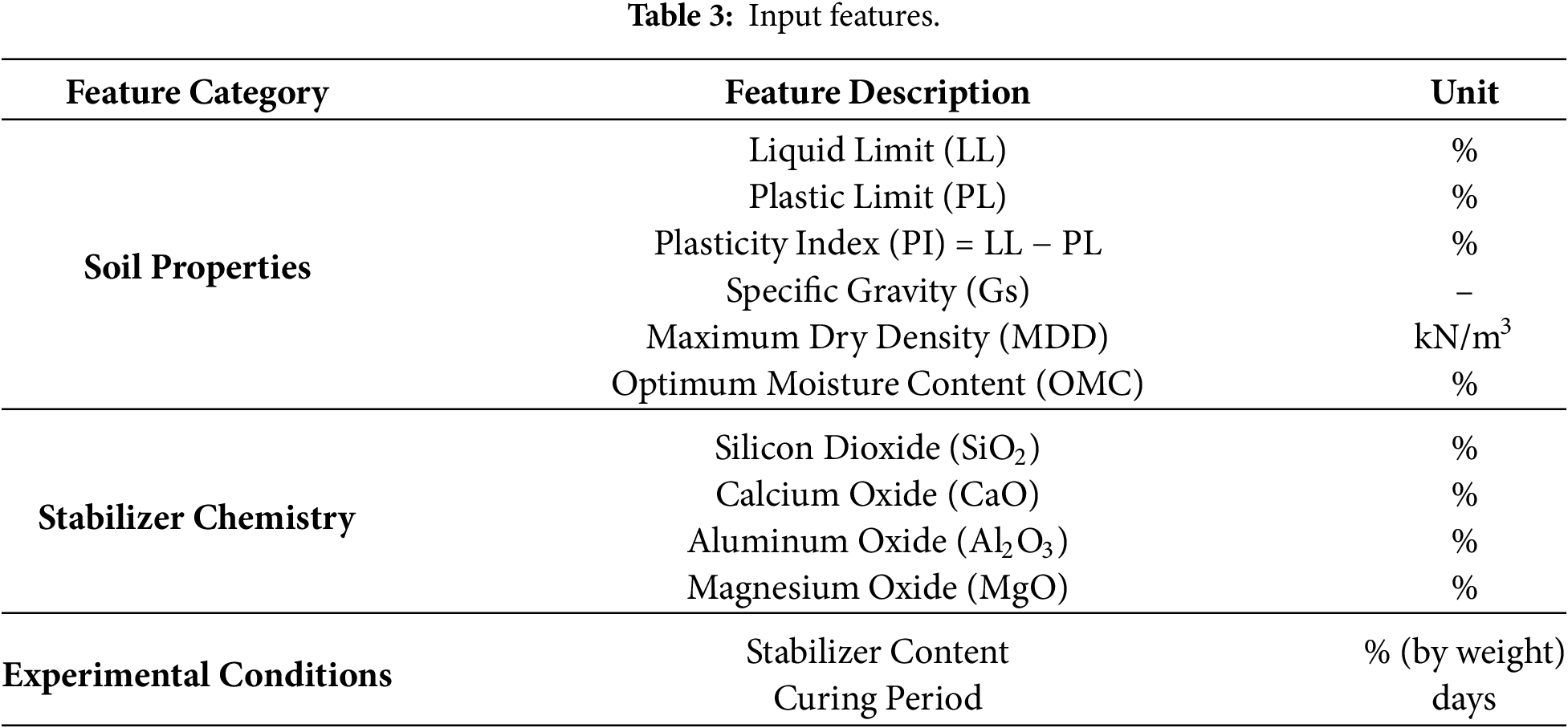
The dataset used in this study comprises experimental data collected from various published research conducted on different types of soils stabilized with different stabilizer. The total number of data were 476 collected from 24 papers as shown in Table 2. The data includes a total of 12 input features encompassing geotechnical properties of untreated soils, chemical compositions of stabilizers, and experimental parameters such as curing period and stabilizer content, the details are shown in Table 3. The target variable is the Unconfined Compressive Strength (UCS), measured in MPa.

2.2 Machine Learning Models

Five supervised machine learning models Random Forest (RF), Gradient Boosting (GB), Extreme Gradient Boosting (XGB), CatBoost, and k-Nearest Neighbors (KNN) were implemented using Scikit-learn, XGBoost, and CatBoost libraries in Python.

2.2.1 Random Forest

RF is a powerful ensemble learning method that creates numerous decision trees upon training and outputs either the class mode (classification) or the average prediction (regression) of the constituent trees. It suits modeling non-linear relationships and coping with high-dimensional data, which is why it is highly suited to predict geotechnical properties such as the UCS of soils [44]. In RF, each tree is learned from a bootstrap sample of the data, and for every node, a random subset of features is considered for splitting. This decorrelation between trees reduces overfitting and enhances generalization performance [19].

In geotechnical engineering, RF has made better predictions in shear strength estimation, settlement, and other mechanical properties since it is able to recognize nuanced interactions between soil characteristics and stabilizer contents [16]. The method does not require significant data preprocessing and is able to handle continuous and categorical variables without standardization, giving a big advantage in heterogeneous soil datasets. Furthermore, RF provides internal variable importance estimates, so it can be applied for feature selection and sensitivity analysis [45].

RF is employed in this study to mimic UCS from 12 input parameters, such as geotechnical indices, chemistry of the stabilizer, and curing conditions. The model is trained using optimized hyperparameters (i.e., depth, number of trees) and cross-validated using R2, RMSE, MAE, and MSE. RF’s ensemble nature entails robustness against outliers and noise, which is an asset in dealing with heterogeneously behaving soil-stabilizer interactions.

2.2.2 Gradient Boosting

Gradient Boosting (GB) is a very successful ensemble technique that creates additive predictive models by fitting a series of weak learners, typically decision trees, in a greedy stage-wise manner such that each tree in the series rectifies the mistakes of its predecessors. GB uses the gradient of the loss function to guide the learning process, and this makes it especially well-adapted to modeling complex, non-linear relationships in data.

Due to its flexibility, GB has been widely applied to regression problems in geotechnical engineering, including UCS and settlement behavior prediction [46]. One of the advantages of GB is that it is able to optimize any differentiable loss function, so it is more robust to skewed data and outliers compared to traditional regression techniques. In this study, GB was trained on soil plasticity indices, chemical composition of stabilizers, and curing conditions.

2.2.3 Extreme Gradient Boosting

XGB is an extremely optimized and state-of-the-art variant of gradient boosting, with its distinguishing factors being scalability, regularization capacity, and computational performance. It improves the efficiency of traditional gradient boosting by adding the incorporation of second-order derivatives of the loss function and regularization terms to punish model complexity, hence reducing the risk of overfitting. This makes it extremely efficient in handling large and complex data sets [47].

XGB also includes native mechanisms for handling missing data and supports parallel processing, which improves training speed and efficiency. It has demonstrated superior predictive performance in soil behavior modeling, including the estimation of undrained shear strength, compressibility, and UCS under varying material compositions and curing conditions [48]. In addition, it provides robust feature importance rankings that align well with SHAP-based interpretability frameworks, making it particularly useful for model explanation.

Its application in geotechnics is growing due to its adaptability to heterogeneous datasets and strong generalization, even when trained on relatively small samples. However, it needs careful regularization and tuning to avoid overfitting. In this paper, XGB is used to predict the UCS of stabilized soils using 12 predictive features.

2.2.4 CatBoost

CatBoost is a machine learning algorithm specifically designed to handle categorical features efficiently. It is a variant of gradient boost that employs binary decision trees as base learners [49]. The algorithm constructs models in an iterative manner, where each new tree is added to correct the errors of the previous approximation. This additive process reduces prediction errors and improves the overall accuracy of the model.

Formally, given a dataset D={(Xj,yj)}j=1m, where Xj is a vector of input characteristics and yj is the corresponding target (binary or numerical), the objective is to train a function H: Rn → R that minimizes a smooth loss function L. At each iteration, CatBoost adds a new function (tree) to the current model using gradient-based optimization methods such as gradient descent or Newton’s method [50,51].

A distinctive strength of CatBoost lies in its ordered boosting technique, which effectively reduces overfitting, and its ability to natively process categorical variables without the need for extensive preprocessing. These features make CatBoost more robust than traditional boost methods such as GB and XGB, especially in datasets with a mix of numerical and categorical inputs [49]. Comparative studies, such as those by Ibrahim et al. [52], have also shown that CatBoost often achieves higher accuracy and stability than other classifiers in various domains. In summary, CatBoost combines the advantages of gradient boosting with innovations for categorical data handling, providing a reliable, interpretable, and high-performance solution for both classification and regression tasks.

2.2.5 K-Nearest Neighbors

The K-Nearest Neighbors (KNN) algorithm is a non-parametric, instance-based learning method used for both classification and regression. In the context of regression, such as predicting UCS, KNN estimates the output value of a query point based on the average of its k nearest neighbors in the feature space.

KNN is simple, intuitive, and effective when relationships between features and outputs are highly non-linear. However, it is sensitive to irrelevant or noisy features and benefits significantly from feature selection and dimensionality reduction, which makes it complementary to SHAP based approaches in geotechnical modeling [53].

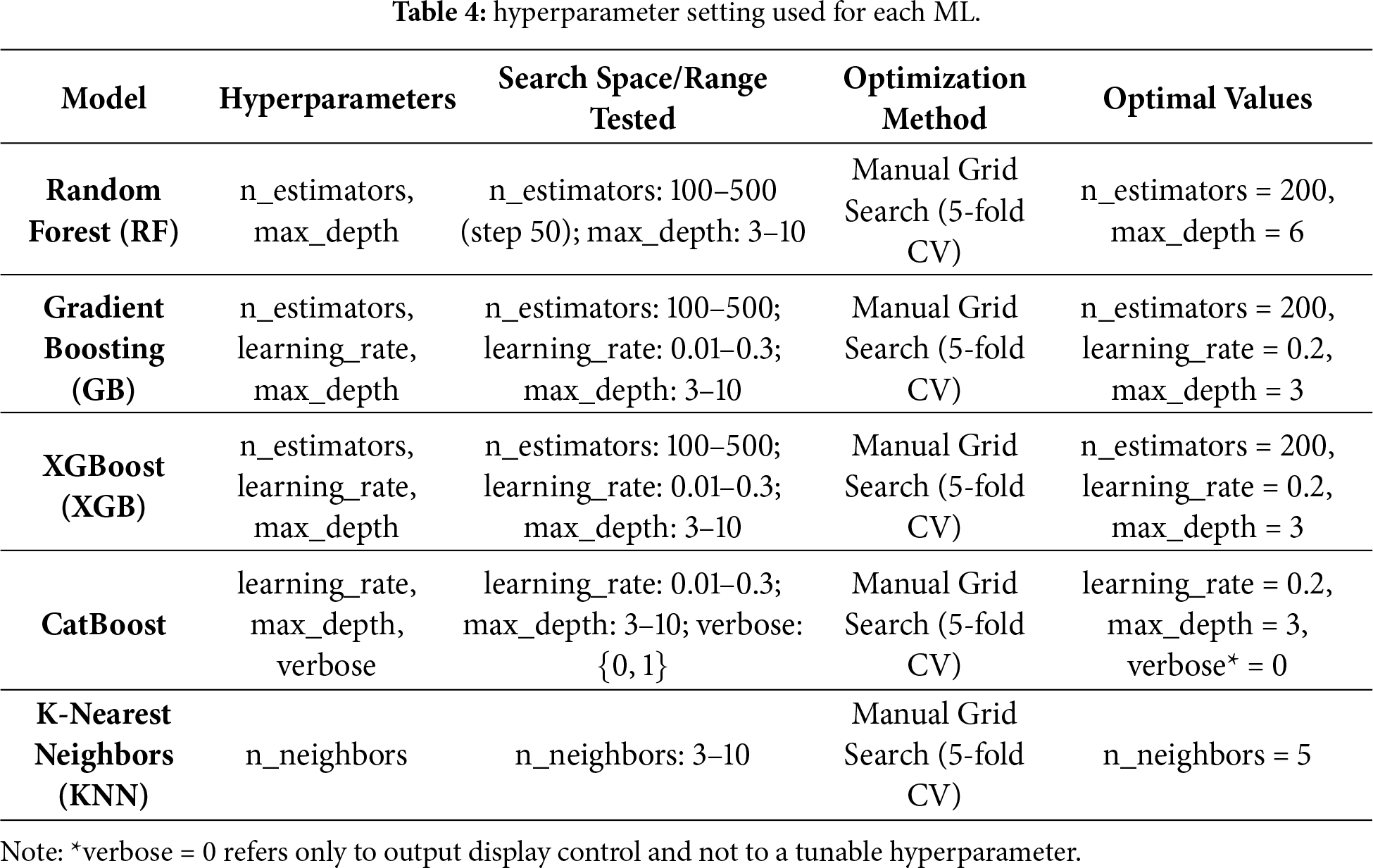
Table 4 shows the hyperparameter setting used for each ML.

2.3 Feature Selection and Reduction Protocol

SHAP (SHapley Additive exPlanations) analysis was utilized to interpret the models and assess the contribution of each feature to the prediction. SHAP offers a cohesive metric of feature significance by assessing the marginal contribution of each input variable to the predicted outcome. The following equation are used to conduct SHAP analysis.

Gj = Gbase + f(Yj1) + f(Yj2) + … + f(Yjk)

Yj = jth specimen.

Yjk = The kth feature of the jth specimen.

Gj = The model’s prediction for this specimen.

Gbase = The baseline of the model.

f(Yjk) = The SHAP value of Yjk.

The subsequent analyses of interpretability based on SHAP were performed:

•   SHAP summary plots to ascertain the principal contributing features.

•   Utilization of dependence plots to elucidate the impact of specific features on UCS.

•   Feature ranking was conducted using SHAP values obtained from the optimal model.

•   To enhance model interpretability and understand how the dimension reduction impacts predictive performance, post-modeling SHAP analysis was conducted. SHAP values are a numerical representation of the extent to which each input feature contributes to the model prediction, based on cooperative game theory.

The mean absolute SHAP values were used to determine global importance, and based on this ranking, the top 8 and top 5 features were selected and uniformly applied to all five ML models for consistent comparison. These reduced feature sets were then used to retrain and re-evaluate all five ML models.

The three input cases examined were:

•   Case A: All 12 original input features

•   Case B: Top 8 features from SHAP importance

•   Case C: Top 5 features from SHAP importance

This approach enabled the performance deterioration (or gain) of the model when using less but more influential features to be studied.

To validate the SHAP-based feature ranking, Random Forest feature importance analysis was also performed. This method quantifies each feature’s contribution to reducing prediction error within the ensemble model, providing an independent check on variable influence. The resulting rankings were compared with SHAP outputs to ensure consistency and robustness in feature selection.

2.4 Model Evaluation

Model evaluation was performed using both an 80/20 train and test split and 5-fold cross-validation, with performance assessments using Coefficient of Determination (R2), Root Mean Squared Error (RMSE), Mean Squared Error (MSE), and Mean Absolute Error (MAE) metrics. These metrics were used to evaluate the machine learning models’ predictive accuracy and generalization ability [54].

These metrics yield complementary information about the performance of the model:

•   R2 reports the proportion of variance in the target variable that is explained by the model.

R2=1−∑i=1n(yi−yi^)2∑i=1n(yi−y−)2

•   RMSE is sensitive to outliers and penalizes larger errors more harshly.

RMSE=1n∑i=1n(yi−yi^)2

•   MSE provides the average squared difference between predictions and actual values.

MSE=1n∑i=1n(yi−yi^)2

•   MAE gives the mean absolute magnitude of prediction errors, giving an interpretable measure of error scale.

MAE=1n∑i=1n|yi−yi^|2

These metrics were computed using the training and testing dataset to ensure unbiased estimation of each model’s predictive performance. The evaluation enabled quantitative comparison between different algorithms and input feature configurations.

2.5 Comparative Analysis

A comprehensive comparative study was performed to observe how every model performed under different feature set scenarios. The comparison framework included:

•   Inter-Model Comparison: Comparing and ranking all five algorithms (RF, GB, XGB, CatB, and KNN) on all four metrics across the three feature sets.

•   Intra-Model Feature Dimensionality Reduction Comparison: Within each model, a performance comparison was conducted for the full (12), reduced-8, and reduced-5 feature sets to study how sensitive the model was to input dimensionality reduction.

•   Performance Stability Analysis: Examining if models with high performance retained predictive capability with fewer features, and seeking significant change in R2 or error measures (RMSE, MSE, MAE) that could be utilized to conclude model robustness and feature importance.

3  Results and Discussion

3.1 Data Distribution, Statistical Summary, and Correlation Heatmap

Before model training, the dataset was explored to understand the statistical characteristics and relationships between the variables Fig. 2 shows the data distribution for all features.

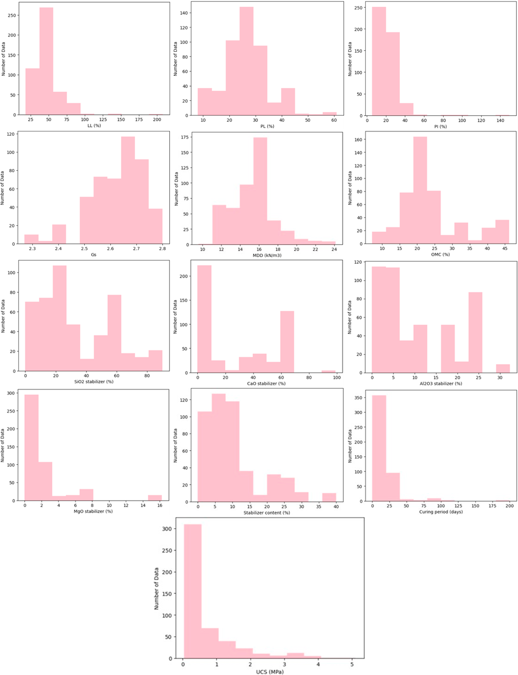
Figure 2: Distribution of the data collected.

The data set has a broad spectrum of soil index properties, chemical mixtures of stabilizers, and processing conditions, each with distinct statistical characteristics. For soil index properties, both LL and PI are highly right-skewed, that is, most soils would have moderately plastic values but there are quite a number with very high plasticity values and these would presumably be highly expansive clays. The PL distribution is symmetrical and suggests even representation of soils with varying plasticity thresholds. Gs values are closely grouped around 2.65, typical of mineral soils, and reflect relatively even mineral composition within samples. The MDD is bell-shaped with a median of 16 kN/m3 that reflects the compaction behavior of the database soils in general, while the OMC is close to normal with a good equilibrium of moisture content for best compaction.

In terms of chemical composition of stabilizers, the Al2O3 and SiO2 percentages appear to be uniformly distributed, suggesting the use of an extremely wide range of stabilizers, possibly natural pozzolans, fly ash, and various industrial by-products. CaO and MgO percentages, however, are highly right-skewed, with majority of stabilizers contributing small content and a smaller fraction having extremely high proportions, probably from lime or cement-based binders. This uneven distribution implies tremendous differences in chemical reactivity among the stabilizers used.

For stabilizer process variables, the content of the stabilizer is significantly right-skewed, with most of the experiments involving low to medium dosages and fewer cases involving high contents. Similarly, the distribution of curing period is significantly right-skewed, with short curing times being the dominant practice while long-term curing trials are much less common. These are symptomatic of normal laboratory, where lower binder content and shorter curing times are usually preferred as a result of cost and time factors.

Finally, the target variable UCS is extremely right-skewed. Most samples have reasonably low strengths, while others achieve high UCS values in excess of 3 MPa, presumably due to combinations of high levels of binder, extended curing times, and favorable chemical content. Skewness is an issue for predictive modeling since value-sensitive algorithms, such as KNN, might be improved by transformations or normalization. Furthermore, the broad range of stabilizer chemistry and processing conditions suggests that feature importance analysis using SHAP can reveal significant and possibly non-linear influences of some chemical and procedural factors on UCS.

The statistical summary in Table 5 shows that the LL averages 46.68% but can reach as high as 208%, indicating a few soils with extremely high plasticity. The PL is more moderate, averaging 26.41% with a maximum of 61%, while the PI averages 20.33% but extends up to 149.6%, confirming a wide range in plasticity characteristics. Gs remains stable around 2.62 with minimal variation. For compaction characteristics, MDD averages 15.31 kN/m3, ranging from 9.6 to 24.13 kN/m3, while OMC averages 23.85%, with most values between 18.7% and 25.5% but some as high as 46.2%.

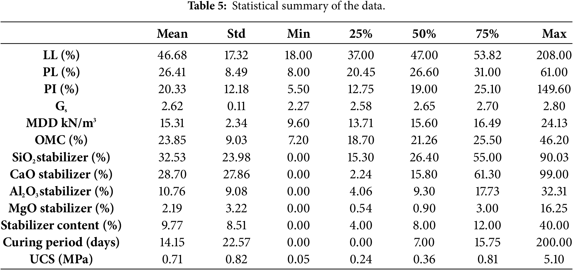
The stabilizer chemical composition varies considerably: SiO2 averages 32.53% (0%–90%), CaO averages 28.70% but reaches 99%, Al2O3 averages 10.76% (0%–32%), and MgO averages just 2.19% but can reach 16.25%. This highlights the diversity in stabilizer materials. In terms of treatment variables, stabilizer content averages 9.77% but ranges from 0% to 40%, while curing period averages 14.15 days but extends up to 200 days, showing large differences in treatment protocols.

The target variable, UCS, has a mean of 0.71 MPa, with most values below 1 MPa but some reaching 5.1 MPa, indicating that while most samples achieve modest strength, a few achieve very high improvements.

The Pearson correlation heatmap between variables in Fig. 3 shows strong and weak linear relationships between the variables of the dataset. Of all the soil index properties, LL, PL, and PI are strongly correlated with one another. LL has strong positive correlations with PI (0.89) and PL (0.76) such that soils with high liquid limits have corresponding high plasticity values. The association of PL–PI is fairly good (0.38), albeit less than for LL–PI. The high interdependence suggests potential multicollinearity of these parameters, so that they may provide redundant information in predictive analysis.

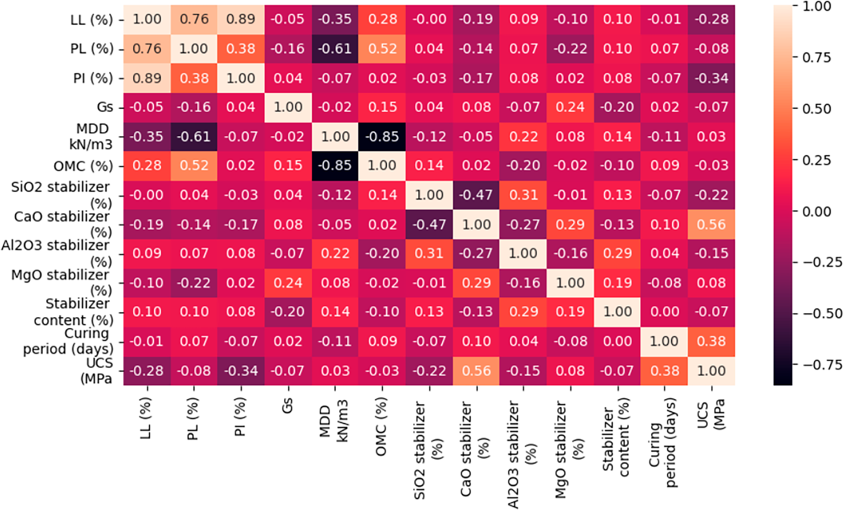
Figure 3: The corelation between the variables.

There is a very high negative correlation between MDD and OMC (−0.85). This would be expected from fundamental soil mechanics principles, in which soils requiring more water for compaction would have lower maximum dry densities. There is even a reasonable correlation between OMC and PL (0.52), indicating that plastic limit rise requires more water for compaction.

For the target variable, UCS is most positively correlated with Al2O3 stabilizer content (0.56) and second-most positively correlated with curing period (0.38). This means that the use of alumina-rich stabilizers and extended curing times are associated with greater strength development. The other oxide phases such as SiO2, CaO, and MgO also have poor direct correlations with UCS and could have less straightforward and potentially non-linear effects on strength and hence are good targets for SHAP-based explainable AI analysis.

Certain moderate correlations are also seen between stabilizer chemistry parameters. SiO2 content is moderately negatively related to CaO (−0.47), which is consistent in the compositional character of stabilizers in which silica-containing materials are also low in calcium. MgO weakly correlates with MDD (0.24), which could suggest denser stabilizer materials.

In general, the heatmap indicates that certain parameters like Al2O3 content and curing time have clear linear relationships with UCS, but others may only affect indirectly through interaction or non-linear effects. The correlations between LL, PL, and PI are high, indicating redundancy and serving as justification for their removal during the 8-feature and 5-feature model test phases.

3.2 Model Performance with All Features

The performance metrics for the 12-feature models show clear differences in predictive accuracy and generalization ability across the five algorithms as shown in Table 6 below.

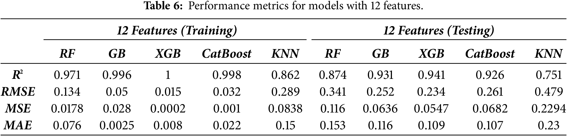
For the training process, all ensemble models (RF, GB, XGB, CatBoost) worked exceedingly well on R2, with XGB having a perfect 1.0, followed closely by CatBoost (0.998), GB (0.996), and RF (0.971). They are all boosted with extremely low RMSE, MSE, and MAE, indicating very minimal prediction errors in training. KNN, though still performing relatively well (R2 = 0.862), falls behind the ensembles with higher RMSE (0.289) and MAE (0.15), which means that it is less able to catch the complex relationships in data.

On testing, performance rankings are slightly changed as models are given unseen data. GB, XGB, and CatBoost retain high generalization with R2 greater than 0.92 and relatively low errors RMSE ranging from 0.234 to 0.261. RF causes the R2 to drop to 0.874, with slightly increased RMSE (0.341) but light overfitting compared to the boosting models. KNN performs the worst of all, with the least R2 (0.751) and highest testing error metrics (RMSE = 0.479, MAE = 0.23), understandably with its lower relevance to this dataset.

Overall, the results show that the most suitable models for predicting UCS from the 12 parameters are the boosting-based models (GB, XGB, CatBoost) with the optimal trade-off between high training accuracy and good generalization in testing. RF is also competitive but less overfitting-resistant, and KNN is clearly less capable of learning the complex relationships of the data.

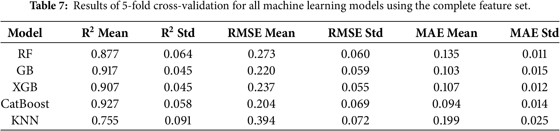
The results of the 5-fold cross-validation shown in Table 7 confirmed the overall robustness and stability of the developed machine learning framework for predicting UCS across different soil–stabilizer combinations. All models exhibited consistent performance with relatively low standard deviations in R2, RMSE, and MAE, indicating that the predictive capability was not dependent on a specific data partition. This demonstrates that the models effectively captured the underlying nonlinear relationships between the input parameters and UCS, achieving reliable generalization across multiple data folds. The close alignment between cross-validated and single split results further validates the soundness of the adopted modeling approach and confirms the absence of significant overfitting, thereby strengthening the empirical reliability of the study’s findings.

3.3 Feature Importance from SHAP Analysis

The SHAP (SHapley Additive exPlanations) method was applied to all the five ML models in an effort to understand the contribution of each input parameter towards UCS prediction as shown in Fig. 4. SHAP provides a single and model-independent approach for interpretation through assessing how much each feature alters the prediction from the baseline value, hence making it highly suitable for complex, non-linear models like RF, GB, XGB, and CatBoost.

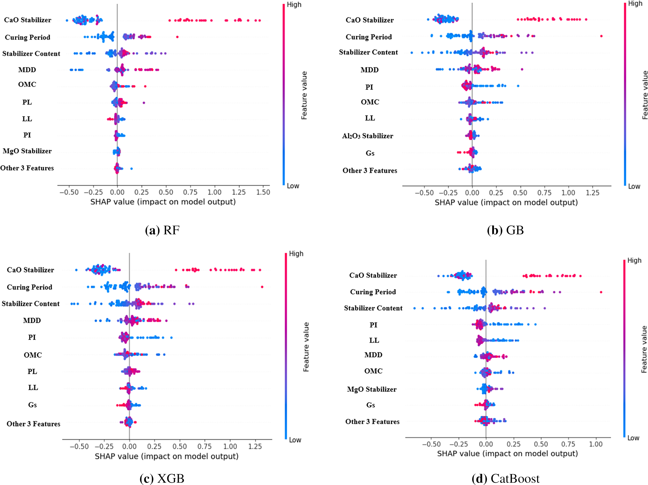
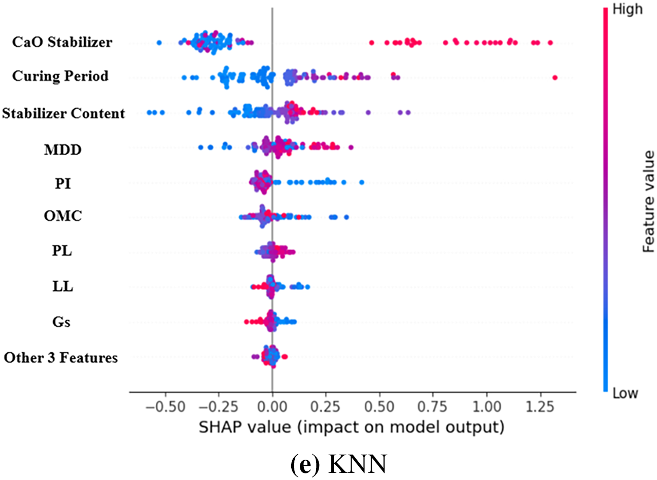
Figure 4: Features importance.

In geotechnical engineering, interpretability at this extent is significant because parameters which most influence mechanical performance are identifiable and can be used to provide insights, which can be linked to known soil stabilization mechanisms.

Table 8 shows feature importance for the models. Across all models, CaO stabilizer content was always the most important characteristic (rank = 1 for all models). Not surprisingly, this dominance exists because calcium-rich stabilizers such as lime and cement play a central role in pozzolanic and cementitious reactions, which contribute directly to UCS by forming calcium silicate hydrates (C–S–H) and other binding phases. Close to CaO, curing time was found to be the second most important parameter in all the models (rank = 2), which is in agreement with the established fact that chemical reaction time and bond development are key factors influencing strength improvement in stabilized soils.

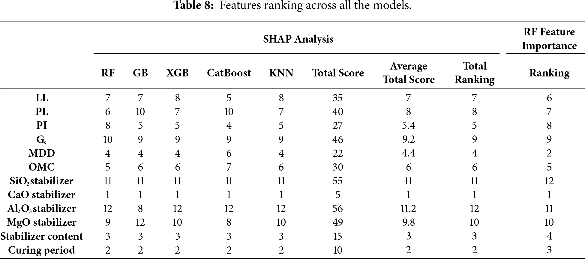
Content of stabilizer was also determined to be the third most important property, indicating that the used dosage of the binder is a crucial parameter of strength gain, although less influential than chemical content (CaO) or reaction time (curing time). MDD came fourth as would be expected from experience where higher compaction density leads to enhanced particle contact and space for the binder reaction with consequent improved UCS.

PI was fifth-ranked in the hierarchy, i.e., clay mineral activity and charge surface properties indirectly dictate stabilization efficiency. OMC came sixth, indicating moisture conditions for optimal compaction and binder hydration. LL and PL were seventh and eighth-ranked, respectively, i.e., even though Atterberg limits are helpful for soil classification, they are less specific for UCS once stabilization parameters are considered.

Those characteristics incorporating Gs (rank 9), MgO stabilizer (rank 10), and SiO2 stabilizer (rank 11) performed less well overall. SiO2’s low ranking is noteworthy because silica content is important in pozzolanic reactions, but reactivity hinges greatly on the presence of CaO and curing conditions, possibly making its individual contribution less significant. The lowest-ranked feature overall was Al2O3 stabilizer content (rank 12), suggesting that alumina plays a less immediate role in strength gain in the datasets tested, or that its effect is trumped by more effective predictors such as CaO and curing time.

The SHAP analysis shows that CaO content, curing period, stabilizer dosage, and MDD positively influence UCS, meaning higher values strengthen the soil. Atterberg limits (LL, PL, PI) negatively impact UCS, as higher plasticity reduces strength, while excessive moisture lowers UCS. MgO and other minor features show weak or inconsistent influence.

From a geotechnical perspective, the SHAP rankings validate domain intuition: strength development is shaped by availability of reactive calcium, binder dosage, and curing time, with compaction properties ranking second. The consistency of rankings across all ML models verifies the robustness of these results and provides strong support to feature selection in subsequent experiments. The top 8 and top 5 features, therefore, that are yielded by these rankings are not arbitrary but are rooted in statistical significance and engineering principles, so reduced-feature models in Section 3.4 are prediction-relevant.

The SHAP analysis indicated that the base value, approximately 0.7 MPa, corresponds to the mean predicted UCS before accounting for individual feature effects. Features such as CaO content, curing period, and stabilizer dosage exhibited positive SHAP values, increasing the prediction above the baseline, whereas parameters like LL and PI showed negative SHAP effects, reducing UCS relative to the base value.

The Random Forest feature importance results closely mirrored the SHAP analysis, confirming the dominance of CaO content, MDD, curing period, stabilizer dosage, and PI as the key determinants of UCS. Minor variables such as LL, PL, MgO, Al2O3, and SiO2 exhibited negligible influence and can therefore be excluded. This agreement between methods reinforces the reliability of the SHAP-guided feature reduction strategy.

3.4 Model Performance with Reduced Features (Top 8 and Top 5)

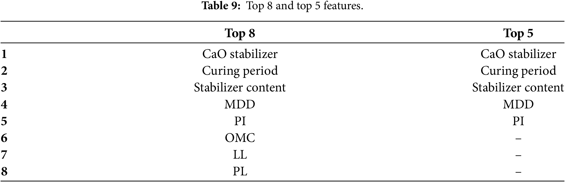
Table 9 shows the top 8 and the top 5 features. The feature reduction process, guided by SHAP importance ranks in Section 3.4, was to examine whether a subsampled set of inputs could maintain high predictive performance for UCS but reduce data acquisition complexity. The selected top 8 and top 5 features represented parameters with highest model-agnostic significance such that the reduced-feature models retained the most influential predictors from both statistical and geotechnical viewpoints.

For the 8-feature models, test R2 values showed minimal loss from the 12-feature baseline. XGB (0.937) and GB (0.938) performed virtually indistinguishably with hardly perceptible increases in RMSE and MSE. CatBoost fell behind by a small margin (R2 = 0.931), which shows great generalization despite feature removal. RF’s test R2 dropped slightly to 0.859, with an increase in RMSE from 0.341 to 0.360, which indicates moderate sensitivity to feature removal. KNN remained the least predictive model (R2 = 0.746), and its already more elevated errors rose slightly than the full-feature model.

For 5-feature models, cross-validation R2′s remained fairly strong for boosting algorithms: GB (0.941) and XGB (0.940) tied or slightly improved upon their 8-feature results, whereas CatBoost (0.935) also had very good accuracy. RF (0.866) performed similarly to its 8-feature equivalent, showing stability at low features. Notably, KNN rose from 0.746 (8 features) to 0.790 (5 features) in R2, suggesting that reducing fewer contributory features reduced noise for this distance-based measure. Despite such strong findings, slight rises in RMSE and MAE in all the models indicated predictive accuracy was slightly affected by the diminishing feature set. Fig. 5 shows the performance metrics and compares between them.

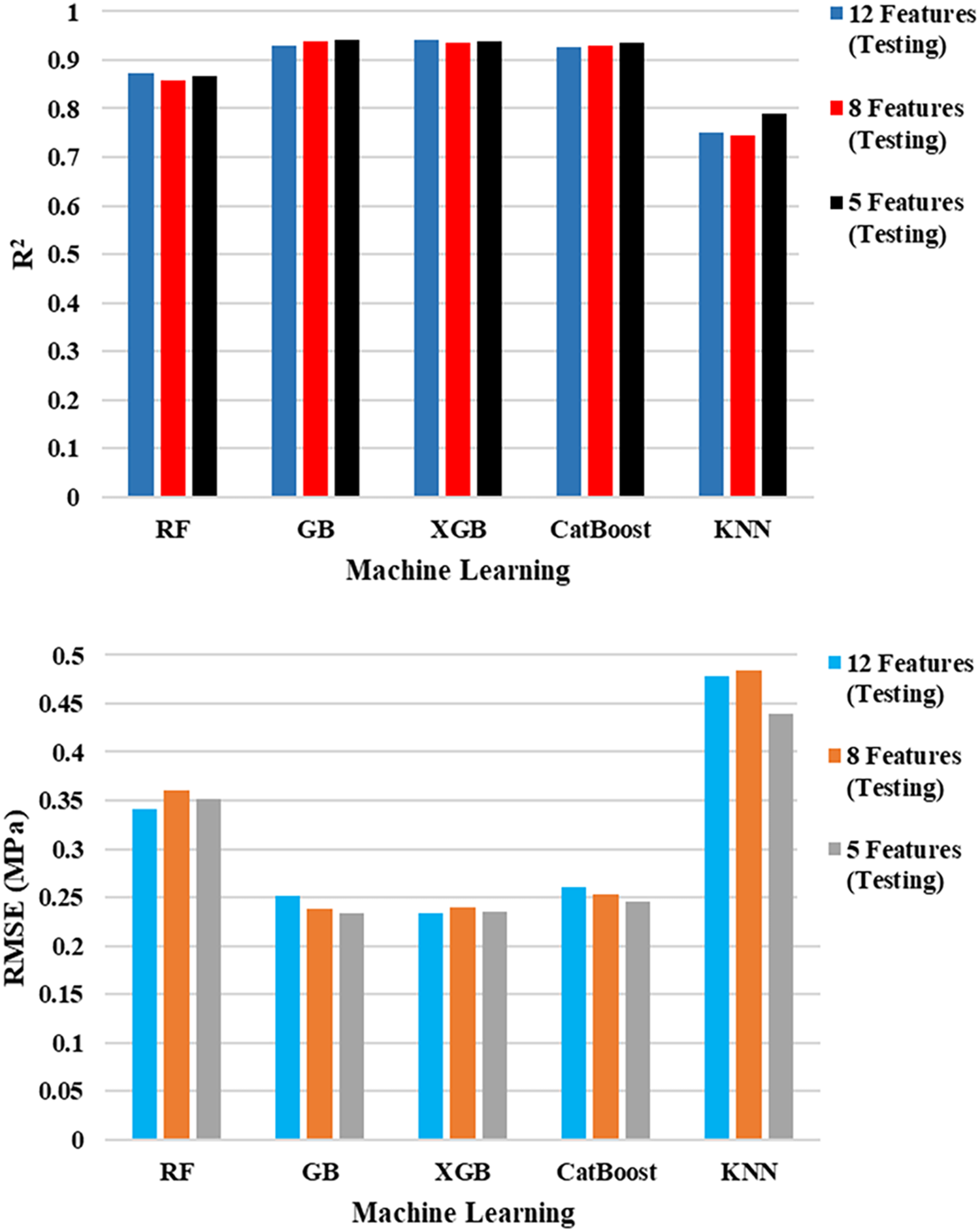
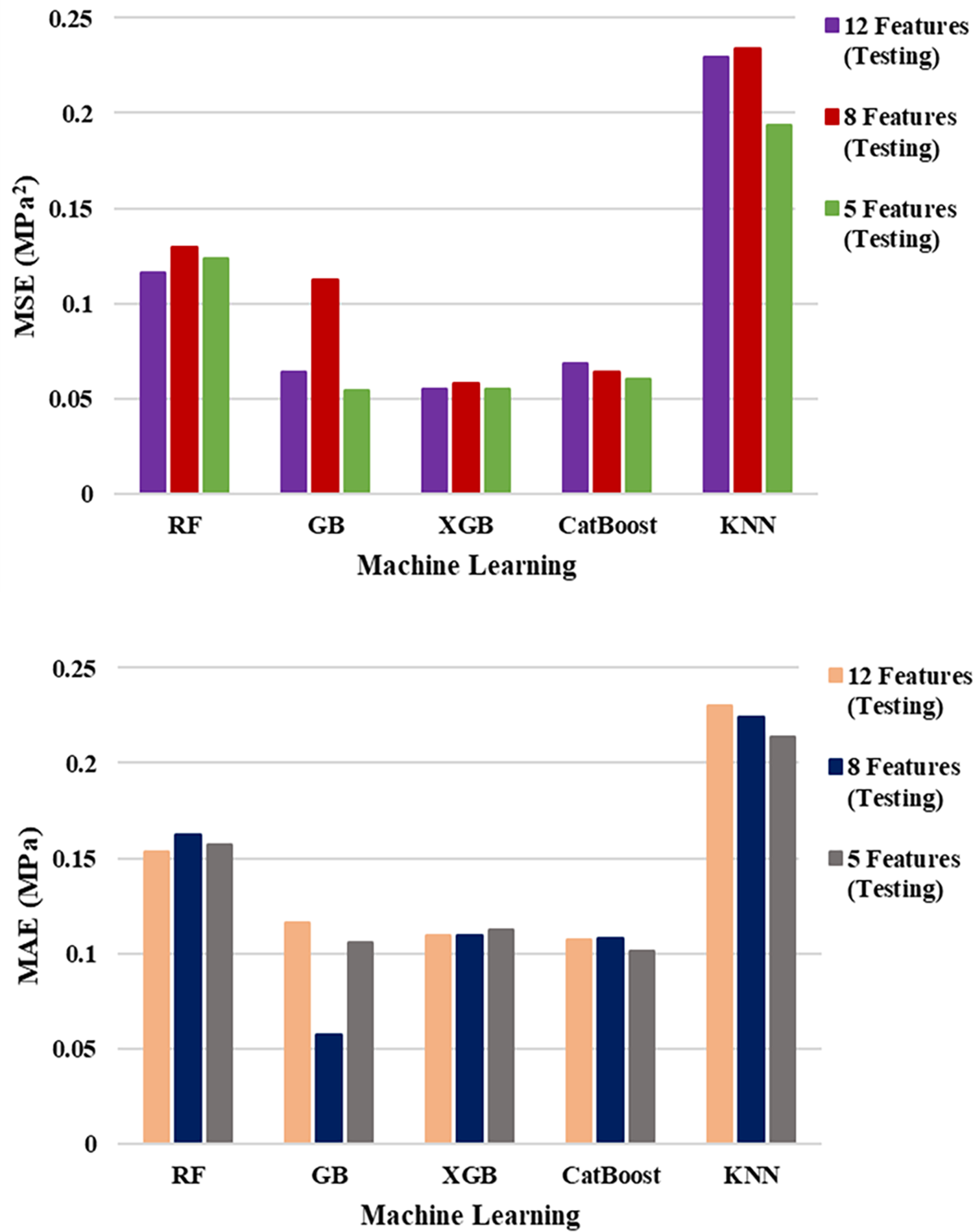
Figure 5: Comparison between performance metrics for the 3 cases (12, 8 and 5 features).

GB, XGB, and CatBoost training metrics were nearly error-free across all feature sets, with tiny increases in error when reducing. XGB still recorded nearly error-free training scores (R2 ≥ 0.999), confirming the ability of XGB to fit the data with unparalleled precision. While tiny deviations between training and testing R2 for boosted models suggest that they did manage to retain generalization potential despite the reducing the number of the inputs. RF and more so KNN experienced a wider train–test gap, as was to be anticipated with their reduced ability to approximate complex non-linear relationships.

Across all three feature configurations, the ranking of performance by model remained constant, with GB and XGB having essentially interchangeable test accuracy in the lower feature sets, though GB slightly outperforming XGB in RMSE for the 5-feature model. CatBoost was in second place close behind, with slightly worse R2 scores but comparable error scores, and therefore a good if not better alternative to GB and XGB. RF was moderately decreasing in performance from 12 to 8 features but remained relatively flat from 8 to 5 features, having some resistance to reduction. KNN was always the worst-performing model overall; however, it was assisted by feature reduction, particularly for the 5-feature set, as removing dimensionality noise that hurts distance-based algorithms must have helped. KNN performance is strongly influenced by the curse of dimensionality, as the algorithm relies on Euclidean distance to measure similarity between data points. In high-dimensional spaces, the relative distances between samples become less discriminative, which degrades KNN accuracy. By reducing the number of input features from 12 to 8 and 5 through SHAP-based feature selection, the model experienced reduced dimensional noise, allowing distance computations to become more meaningful and improving local neighborhood structure identification. Consequently, the KNN algorithm could better capture the true proximity relationships between samples, leading to observable performance gains.

Performance stability in reduced-feature versions also follows the SHAP rankings, whereby top-ranked features (CaO content, curing time, stabilizer content, MDD, and PI) all have significant theoretical correlations with UCS formation. Omitting lower-ranked but, in some chemical contexts, useful features such as SiO2, Al2O3, and MgO did not significantly affect prediction capability, presumably because they were indirectly covered by prevailing parameters. This finding has real-world implications: it means that UCS predictive models can be very accurate with fewer, simpler-to-measure parameters, at lower cost and effort for testing, without sacrificing performance.

Based on the SHAP global importance results, the five most influential features for UCS prediction were identified as CaO content, curing period, stabilizer dosage, MDD, and PI. These parameters consistently exhibited the highest SHAP values across all machine learning models, confirming their dominant role in controlling soil strength development. The remaining features: LL, PL, OMC, SiO2, Al2O3, MgO, and Gs, showed negligible contributions and can therefore be safely excluded without compromising model performance. From an engineering perspective, retaining only the top five predictors offers a more practical and cost-effective approach, reducing the need for extensive laboratory testing while maintaining reliable UCS prediction accuracy for stabilized soils.

The comparison quite visibly shows that prediction performance can be maintained with as few as 5 well-selected features. For this data, GB and XGB with 5 features had similarly excellent performance to their 12-feature versions, with R2 ≈ 0.94 and only modest increments in error measures. This outcome fulfills the research’s primary objective, showing that feature selection based on SHAP facilitates model simplification without sacrifice of predictiveness.

Table 10 shows the difference in performance measures (∆R2 and ∆RMSE) with a reduction in the number of input features from 12 to 8 and 5. These results show that the effect on accuracy was very small for all models, with ΔR2 always being below 0.02 and only slight, inconsiderable increases in RMSE values. In certain models, including GB and CatBoost, even a slight improvement in performance was observed, which supports the fact that the models performed satisfactorily despite the reduction in features. This observation clearly shows that both the 8-feature and 5-feature models performed for predictive purposes with identical configurations. From an implementation perspective, any reduction in input features resulted in substantial cost and time-saving advantages, with reduced analytical work required in laboratories for precise predictions related to UCS values. Thus, SHAP values offered not only improved understandability but also created a cost-effective method that performs accurately in the lab.

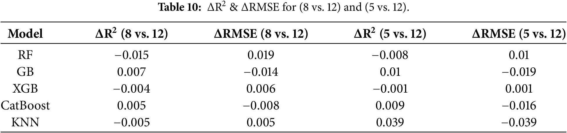
To statistically assess whether the observed differences in model performance across feature configurations were significant, paired t-tests were conducted using RMSE values from the 12-, 8-, and 5-feature models. The results showed no statistically significant difference between configurations, with t = −0.2766 and p = 0.7958 for the 12 vs. 8 features comparison, and t = 1.4823 and p = 0.2124 for the 12 vs. 5 features comparison. Since both p-values exceed 0.05, the null hypothesis of equal performance cannot be rejected, indicating that the reduction in input features does not significantly affect model accuracy. This finding confirms that the SHAP-guided feature reduction approach maintains predictive reliability while minimizing the number of laboratory tests required for UCS estimation.

4  Conclusion

This study presented a holistic framework for the prediction of Chemically Stabilized Soil Unconfined Compressive Strength (UCS) using five machine learning models RF, GB, XGB, CatBoost, and KNN with SHAP-based interpretability and dimensionality reduction. The 12 geotechnical and chemical parameters were considered in the dataset, and SHAP was used to identify the most important predictors. The models were re-trained using top 8 and top 5 features and compared to the full-feature models based on R2, RMSE, MSE, and MAE.

Results indicated that gradient boosting algorithms provided the highest accuracy across all feature settings, with little loss of accuracy when truncated to 8 or 5 features. SHAP rankings revealed good agreement with traditional geotechnical knowledge, emphasizing the effects of curing time, stabilizer content, specific gravity, and plasticity ratios on UCS. This confirms that low-feature models could offer comparable accuracy to high-feature models but limit data acquisition costs and increase interpretability, making them viable for engineering applications where productivity is most critical. The major conclusions are:

•   SHAP-driven feature reduction effectively ranked most influential UCS predictors according to geotechnical theory.

•   Gradient boosting models (GB, XGB, CatBoost) maintained R2 > 0.93 in test even with only 5 features.

•   Low loss in accuracy from 12 to 8 or 5 features for top models supports cost-effective predictive workflows.

•   RF remained competitive but more adversely affected by feature reduction.

•   KNN improved slightly with feature reduction because of lower dimensional noise.

•   The framework presents a best balance of accuracy, interpretability, and data efficiency to make it worthy of more extensive utilization in geotechnical practice.

•   Although the developed models performed well, certain limitations should be noted. The dataset was compiled from multiple studies, which may introduce inter-study variability and bias due to differing soil and stabilizer conditions. Statistical significance testing of performance differences was not conducted in this work. These limitations highlight opportunities for future studies to enhance generalization and practical deployment.

Acknowledgement: Not applicable.

Funding Statement: The authors received no specific funding for this study.

Author Contributions: The authors confirm contribution to the paper as follows: Ahmed Mohammed Awad Mohammed: Conceptualization, Methodology. Ahmed Mohammed Awad Mohammed, Omayma Husain: Investigation, Formal analysis. Ahmed Mohammed Awad Mohammed, Abdalmomen Mohammed: Software, Validation, Visualization. Ahmed Mohammed Awad Mohammed, Omayma Husain, Mosab Hamdan: Writing—original draft. Abdullah Ansari, Atef Badr, Abubakar Elsafi, Abubakr Siddig: Writing—review & editing. All authors reviewed and approved the final version of the manuscript.

Availability of Data and Materials: The data that support the findings of this study are available from the Corresponding Author, upon reasonable request.

Ethics Approval: Not applicable.

Conflicts of Interest: The authors declare no conflicts of interest.

References

1. Jamaludin N, Mohd Yunus NZ, Mohammed AMA, Haron Z, Marto A, Mashros N, et al. Comparison between cement and concrete waste on the strength behaviour of marine clay treated with coal ash. MATEC Web Conf. 2018;250(1):01003. doi:10.1051/matecconf/201825001003. [Google Scholar] [CrossRef]

2. Mohammed AMA, Almthailee YHY, Mohd Yunus NZ, Hezmi MA. Effect of ground granulated furnaces blast slag on kaolin properties. Malays Constr Res J. 2021;13(2):241–52. [Google Scholar]

3. Awad Mohammed AM, Mohd Yunus NZ, Hezmi MA, Rashid ASA, Jusoh SN, Arliansyah J. Effect of voids in kaolin stabilised by ground granulated blast furnaces slag mixtures. IOP Conf Ser Earth Environ Sci. 2022;971(1):012021. doi:10.1088/1755-1315/971/1/012021. [Google Scholar] [CrossRef]

4. Besalatpour A, Hajabbasi MA, Ayoubi A, Gharipour A, Jazi AY. Prediction of soil physical properties by optimized support vector machines. Int Agrophys. 2012;26(2):109–15. doi:10.31545/intagr/103938. [Google Scholar] [CrossRef]

5. Zhang C, Zhu Z, Liu F, Yang Y, Wan Y, Huo W, et al. Efficient machine learning method for evaluating compressive strength of cement stabilized soft soil. Constr Build Mater. 2023;392(8):131887. doi:10.1016/j.conbuildmat.2023.131887. [Google Scholar] [CrossRef]

6. Wang Y, Hasanipanah M, Rashid ASA, Le BN, Ulrikh DV. Advanced tree-based techniques for predicting unconfined compressive strength of rock material employing non-destructive and petrographic tests. Materials. 2023;16(10):3731. doi:10.3390/ma16103731. [Google Scholar] [PubMed] [CrossRef]

7. Cong Y, Motohashi T, Nakao K, Inazumi S. Machine learning predictive analysis of liquefaction resistance for sandy soils enhanced by chemical injection. Mach Learn Knowl Extr. 2024;6(1):402–19. doi:10.3390/make6010020. [Google Scholar] [CrossRef]

8. Ahmad M, Al Zubi M, Almujibah H, Sabri Sabri MM, Mustafvi JB, Haq S, et al. Improved prediction of soil shear strength using machine learning algorithms: interpretability analysis using SHapley Additive exPlanations. Front Earth Sci. 2025;13:1542291. doi:10.3389/feart.2025.1542291. [Google Scholar] [CrossRef]

9. Thisovithan P, Aththanayake H, Meddage DPP, Ekanayake IU, Rathnayake U. A novel explainable AI-based approach to estimate the natural period of vibration of masonry infill reinforced concrete frame structures using different machine learning techniques. Results Eng. 2023;19:101388. doi:10.1016/j.rineng.2023.101388. [Google Scholar] [CrossRef]

10. Lundberg S, Lee SI. A unified approach to interpreting model predictions. In: Proceedings of the Advances in Neural Information Processing Systems; 2017 Dec 4–9; Long Beach, CA, USA. [Google Scholar]

11. Kumar A, Singh V, Singh S, Kumar R, Bano S. Prediction of unconfined compressive strength of cement-lime stabilized soil using artificial neural network. Asian J Civ Eng. 2024;25(2):2229–46. doi:10.1007/s42107-023-00905-w. [Google Scholar] [CrossRef]

12. Kumar A, Sinha S, Saurav S, Chauhan VB. Prediction of unconfined compressive strength of cement-fly ash stabilized soil using support vector machines. Asian J Civ Eng. 2024;25(2):1149–61. doi:10.1007/s42107-023-00833-9. [Google Scholar] [CrossRef]

13. Yao Q, Tu Y, Yang J, Zhao M. Hybrid XGB model for predicting unconfined compressive strength of solid waste-cement-stabilized cohesive soil. Constr Build Mater. 2024;449:138242. doi:10.1016/j.conbuildmat.2024.138242. [Google Scholar] [CrossRef]

14. Priyadarshee A, Chandra S, Gupta D, Kumar V. Neural models for unconfined compressive strength of kaolin clay mixed with pond ash, rice husk ash and cement. J Soft Comput Civ Eng. 2020;4(2):85–102. doi:10.12989/gae.2017.12.1.085. [Google Scholar] [CrossRef]

15. Mozumder RA, Laskar AI, Hussain M. Empirical approach for strength prediction of geopolymer stabilized clayey soil using support vector machines. Constr Build Mater. 2017;132:412–24. doi:10.1016/j.conbuildmat.2016.12.012. [Google Scholar] [CrossRef]

16. Zeini HA, Al-Jeznawi D, Imran H, Almeida Bernardo LF, Al-Khafaji Z, Ostrowski KA. Random forest algorithm for the strength prediction of geopolymer stabilized clayey soil. Sustainability. 2023;15(2):1408. doi:10.3390/su15021408. [Google Scholar] [CrossRef]

17. Ly HB, Pham BT. Soil unconfined compressive strength prediction using random forest (RF) machine learning model. Open Constr Build Technol J. 2020;14(1):278–85. doi:10.2174/1874836802014010278. [Google Scholar] [CrossRef]

18. Chen Q, Hu G, Wu J. Comparative study on the prediction of the unconfined compressive strength of the one-part geopolymer stabilized soil by using different hybrid machine learning models. Case Stud Constr Mater. 2024;21:e03439. doi:10.1016/j.cscm.2024.e03439. [Google Scholar] [CrossRef]

19. Mohammed AMA, Husain O, Abdulkareem M, Mohd Yunus NZ, Jamaludin N, Mutaz E, et al. Explainable Artificial Intelligence for predicting the compressive strength of soil and ground granulated blast furnace slag mixtures. Results Eng. 2025;25:103637. doi:10.1016/j.rineng.2024.103637. [Google Scholar] [CrossRef]

20. Mohamedzein YEA, Al-Rawas AA. Cement-stabilization of sabkha soils from Al-auzayba, sultanate of Oman. Geotech Geol Eng. 2011;29(6):999–1008. doi:10.1007/s10706-011-9432-y. [Google Scholar] [CrossRef]

21. Nasr AMA. Geotechnical characteristics of stabilized sabkha soils from the Egyptian-Libyan coast. Geotech Geol Eng. 2015;33(4):893–911. doi:10.1007/s10706-015-9872-x. [Google Scholar] [CrossRef]

22. Ozdemir MA. Improvement in bearing capacity of a soft soil by addition of fly ash. Procedia Eng. 2016;143:498–505. doi:10.1016/j.proeng.2016.06.063. [Google Scholar] [CrossRef]

23. Parimala BI, Ganesh B, Chitra R. Stabilization of expansive soil using flyash and lime. Int J Curr Eng Sci Res. 2017;4(2):5–10. doi:10.21275/v5i6.nov164333. [Google Scholar] [CrossRef]

24. Ismaiel HAH. Cement kiln dust chemical stabilization of expansive soil exposed at el-kawther quarter, sohag region. Egypt Int J Geosci. 2013;4(10):1416–24. doi:10.4236/ijg.2013.410139. [Google Scholar] [CrossRef]

25. Murugan S, Vijayarangam M. Influence of fly ash to improve the shear strength of commercial and natural soil. Int J Curr Eng Technol. 2014;3:213–6. [Google Scholar]

26. Tamang P, Sriskantharajah A, Ferreira P, Lopez-Querol S. Experimental evaluation of kaolin stabilised with class F fly ash. Bull Eng Geol Environ. 2021;80(9):6781–98. doi:10.1007/s10064-021-02373-5. [Google Scholar] [CrossRef]

27. Saeed KA, Kassim KA, Nur H. Physicochemical characterization of cement treated kaolin clay. Gradjevinar. 2014;66(6):513–21. doi:10.14256/JCE.976.2013. [Google Scholar] [CrossRef]

28. Kandalai S, Patel A. Geomechanical and microstructural behaviour of expansive soil stabilized with red mud and GGBS: an experimental investigation. Arab J Sci Eng. 2025;50(11):7965–85. doi:10.1007/s13369-024-09171-7. [Google Scholar] [CrossRef]

29. Asgari MR, Baghebanzadeh Dezfuli A, Bayat M. Experimental study on stabilization of a low plasticity clayey soil with cement/lime. Arab J Geosci. 2015;8(3):1439–52. doi:10.1007/s12517-013-1173-1. [Google Scholar] [CrossRef]

30. Umar IH, Orakoglu Firat ME. Investigation of unconfined compressive strength of soils stabilized with waste elazig cherry marble powder at different water contents. In: Proceedings of the 14th International Conference on Engineering & Natural Sciences; 2022 Jul 18–19; Sivas, Turkey. [Google Scholar]

31. Hastuty IP. Comparison of the use of cement, gypsum, and limestone on the improvement of clay through unconfined compression test. J Civ Eng Forum. 2019;5(2):131. doi:10.22146/jcef.43792. [Google Scholar] [CrossRef]

32. Roy A. Soil stabilization using rice husk ash and cement. Int J Civ Eng Res. 2014;5(1):49–54. doi:10.53555/ajbr.v27i4s.3704. [Google Scholar] [CrossRef]

33. Rahman MHK, Md Nujid M, Idrus J, Tholibon DA, Bawadi NF. Unconfined compressive strength assessment of stabilized marine soil with cockle shell powder as sustainable material on subgrade pavement. IOP Conf Ser Earth Environ Sci. 2023;1205(1):012057. doi:10.1088/1755-1315/1205/1/012057. [Google Scholar] [CrossRef]

34. Ashraf MA, Rahman SS, Faruk MO, Bashar MA. Determination of optimum cement content for stabilization of soft soil and durability analysis of soil stabilized with cement. Am J Civ Eng. 2018;6(1):39–43. doi:10.11648/j.ajce.20180601.17. [Google Scholar] [CrossRef]

35. Fattah MY, Rahil FH, Al-Soudany KY. Improvement of clayey soil characteristics using rice husk ash. J Civ Eng Urban. 2013;3(1):12–8. [Google Scholar]

36. Alhassan M. Potentials of rice husk ash for soil stabilization. Assumpt Univ (AU) J Technol. 2008;11(4):246–50. [Google Scholar]

37. Islam S, Hoque N, Chowdhury M. Strength development in clay soil stabilized with fly ash. Jordan J Civ Eng. 2018;12(2):188–201. [Google Scholar]

38. Rahgozar MA, Saberian M, Li J. Soil stabilization with non-conventional eco-friendly agricultural waste materials: an experimental study. Transp Geotech. 2018;14:52–60. doi:10.1016/j.trgeo.2017.09.004. [Google Scholar] [CrossRef]

39. Latifi N, Eisazadeh A, Marto A, Meehan CL. Tropical residual soil stabilization: a powder form material for increasing soil strength. Constr Build Mater. 2017;147:827–36. doi:10.1016/j.conbuildmat.2017.04.115. [Google Scholar] [CrossRef]

40. Navagire OP, Sharma SK, Rambabu D. Stabilization of black cotton soil with coal bottom ash. Mater Today Proc. 2022;52:979–85. doi:10.1016/j.matpr.2021.10.447. [Google Scholar] [CrossRef]

41. Dissanayake TBCH, Senanayake SMCU, Nasvi MCM. Comparison of the stabilization behavior of fly ash and bottom ash treated expansive soil. Engineer. 2017;50(1):11. doi:10.4038/engineer.v50i1.7240. [Google Scholar] [CrossRef]

42. Devi CR, Surendhar S, Vijaya Kumar P, Sivaraja M. Bottom ash as an additive material for stabilization of expansive soil. Int J Eng Tech. 2018;4(2):174–80. [Google Scholar]

43. Almuaythir S, Zaini MSI, Hasan M, Hoque MI. Sustainable soil stabilization using industrial waste ash: enhancing expansive clay properties. Heliyon. 2024;10(20):e39124. doi:10.1016/j.heliyon.2024.e39124. [Google Scholar] [PubMed] [CrossRef]

44. Breiman L. Random forests. Mach Learn. 2001;45(1):5–32. doi:10.1023/a:1010933404324. [Google Scholar] [CrossRef]

45. Pham BT, Qi C, Ho LS, Nguyen-Thoi T, Al-Ansari N, Nguyen MD, et al. A novel hybrid soft computing model using random forest and particle swarm optimization for estimation of undrained shear strength of soil. Sustainability. 2020;12(6):2218. doi:10.3390/su12062218. [Google Scholar] [CrossRef]

46. Zhang W, Zhang R, Wu C, Goh ATC, Wang L. Assessment of basal heave stability for braced excavations in anisotropic clay using extreme gradient boosting and random forest regression. Undergr Space. 2022;7(2):233–41. doi:10.1016/j.undsp.2020.03.001. [Google Scholar] [CrossRef]

47. Zhang R, Li Y, Goh ATC, Zhang W, Chen Z. Analysis of ground surface settlement in anisotropic clays using extreme gradient boosting and random forest regression models. J Rock Mech Geotech Eng. 2021;13(6):1478–84. doi:10.1016/j.jrmge.2021.08.001. [Google Scholar] [CrossRef]

48. Zhang W, Wu C, Zhong H, Li Y, Wang L. Prediction of undrained shear strength using extreme gradient boosting and random forest based on Bayesian optimization. Geosci Front. 2021;12(1):469–77. doi:10.1016/j.gsf.2020.03.007. [Google Scholar] [CrossRef]

49. Prokhorenkova L, Gusev G, Vorobev A, Dorogush AV, Gulin A. CatBoost: unbiased boosting with categorical features. Adv Neural Inf Process Syst. 2018;31:1–11. [Google Scholar]

50. Mason L, Baxter J, Bartlett P, Frean M. Boosting algorithms as gradient descent. Adv Neural Inf Process Syst. 1999;12:1–7. [Google Scholar]

51. Friedman J, Hastie T, Tibshirani R. Additive logistic regression: a statistical view of boosting (with discussion and a rejoinder by the authors). Ann Statist. 2000;28(2):337–407. doi:10.1214/aos/1016218223. [Google Scholar] [CrossRef]

52. Ibrahim AA, Raheem L, Muhammed M, Rabiat O, Ganiyu A. Comparison of the CatBoost classifier with other machine learning methods. Int J Adv Comput Sci Appl. 2020;11(11):738–48. doi:10.14569/ijacsa.2020.0111190. [Google Scholar] [CrossRef]

53. Cover T, Hart P. Nearest neighbor pattern classification. IEEE Trans Inform Theory. 1967;13(1):21–7. doi:10.1109/tit.1967.1053964. [Google Scholar] [CrossRef]

54. Wen T, Lin C, Zhang J, Huang D, Chen N. Prediction model for uniaxial compressive strength of rocks based on dual optimization of input parameters and hyperparameters. Transp Infrastruct Geotechnol. 2026;13(1):9. doi:10.1007/s40515-025-00774-7. [Google Scholar] [CrossRef]