Pixel-Level Feature Extraction Model for Breast Cancer Detection

1  Introduction

Cancer is caused by cell abnormalities and is a leading cause of death worldwide. The American Cancer Society (ACS) has estimated that 1.9 million new cancer cases were identified and 608,570 people died of the disease in 2021 in the United States alone (1670 deaths/day) [1]. Breast cancer is the most frequently diagnosed form of cancer [2]. Breast cancer detection is an important but difficult task because symptoms of the disease are not prominent in the early stages. A commonly used technique for detecting cancer is the fine-needle aspiration (FNA) procedure, in which tissues are collected from areas of the body that are likely to be afflicted. FNA is an invasive and painful process but provides accurate results. The extracted tissues are fixed into slides, and the cytoplasm and nuclei are highlighted in different colors through hematoxylin and eosin (H&E) staining. These slides are manually analyzed under a microscope to look for abnormalities that are indicative of cancer. Large digitalized images of these slides are usually obtained at a high resolution, and contain colors of different intensities in different parts. Analyzing the entire image of a slide is time-consuming and, labeling each malignant area is challenging and tedious. Multiple specialists analyze the same images in complex cases and discuss their opinions to reach a consensus. These experts may have different opinions on artifacts present in the same image. Their final diagnoses can differ, and depend on their level of expertise. Computer-aided diagnostics (CAD) systems can be used to analyze digital images by using computer vision and image processing methods. This study proposes an automatic machine learning (ML) based model for the pixel categorization and labeling of images for the diagnosis of breast cancer.

The remainder of this paper is organized into the following sections: Section 2 describes past work in the area of image segmentation, feature extraction, and machine learning. Section 3 details the proposed method, which includes the random forest (RF), decision tree (DT) and extra tree (ET) algorithms as well as feature extraction, genetic algorithm (GA)-based feature selection, and performance-related parameters. Section 4 describes the experimental setup used to test the proposed method, the results, and an assessment of its performance. Section 5 summarizes the conclusions of this study and highlights directions for future work in the area.

2  Literature Review

Researchers have explored solutions for a better, faster, and more accurate understanding of medical images by using computer-based methods. Medical images contain complex patterns that make image processing tasks challenging. In the last decade, many attempts have been made to detect objects in images. Object-oriented algorithms, firefly models, and hybrid models have been developed for the segmentation and classification of nuclei. A recent study [3] extracted the color histogram as well as features of texture and the frequency domain from RGB images to identify periocular cancer. Another study [4] used four hybrid algorithms for segmentation: K-means, fuzzy C-means, the comparative learning-based neural network, and Gaussian mixture. The competitive learning method attained the highest accuracy (96%) among them. The authors applied the Inception v3 model for feature extraction in a study on the segmentation of lesions [5], extracted gradient-based features from dermoscopic images, and used them for classification with an accuracy of 99.2%. Yet another study [6] used CAD for the detection of skin cancer and extracted unique features from the segmented images of lesions. Lesions in the case of melanoma exhibit variations in color while benign skin has a uniform color. Therefore, color-, shape-, and texture-based features are commonly extracted from images of the skin for diagnosis. The extracted features are then processed to reduce noise in them as well as their dimensionality. A popular method for region segmentation involves identifying pixels with similar values. Researchers [7] have proposed an object-oriented method for measuring the homogeneity of images obtained during the biopsy of the colon by using the distributions of objects in the images. The texture is a fundamental and low-level characteristic that is used to discern the contents and patterns in an image. These characteristics are beneficial for partitioning distinct regions that have the same color. Textural characteristics in ultrasound images are used to diagnose prostate cancer [8–10]. The textural analysis of PET images has also been explored [11], and the authors concluded that textural characteristics are beneficial for tumor detection. Geometric characteristics have been used to locate the internal cervical OS [12]. A study [13] used high-order spectra (HOS) and the local binary pattern (LBP) to identify cases of oral cancer. The authors [14] have utilized an ultrasound scanner to analyze the textural properties of images to identify cysts. They found that the co-occurrence matrix was suitable for this task. morever a study [15] retrieved color-and texture-based characteristics from images of patients with meningioma. A study on segmentation [16] focused on detecting breast cancer lesions using texture descriptors. Another studies [17,18] exhibited textural characteristics collected from sub-images to classify breast cancer as benign or malignant. These textural elements were used to obtain average values of images with the same distances between pixels in four distinct orientations. In the reference [19], textural characteristics have been extracted using different filters, the gray-level co-occurrence matrix, and the local properties of images. The feature set thus obtained was used for computer-based breast cancer screening. Traditional techniques of classification include statistical analysis, support vector machine (SVM), artificial neural network (ANN), decision tree (DT), random forest (RF), and K-nearest neighbor (KNN). In a primary study [20], the authors applied four classifiers—one-nearest neighbor (1NN), quadratic linear analysis (QDA), SVM, and RF—to classify histological images of tumors in the breast ether as benign or malignant. Another study [21] assessed the performance of the KNN and ANN classifiers, where the latter outperformed the former. A research paper [22] experimented with a KNN classifier to extract shape-and co-occurrence-based features from a mammography dataset for classification. This method attained an accuracy of 82% under the ROC curve, which is unsatisfactory. Researchers [23] have also developed an automated system for cancer diagnosis and classification by using images obtained during biopsies. It covers a range of necessary tasks from pre-processing to classification, where adaptive histogram equalization was used in the pre-processing, K-means clustering was used for segmentation, and the fuzzy KNN, SVM, and RF algorithms were used for classification. The results of their experiments showed that the KNN is the most accurate model. In recent work, the authors segmented images of the lung and identified the airway in it by using morphological operations. They reduced error by using optimal thresholding on grayscale images [24].

Although the above results are promising there is still room for improvement in feature extraction and reduction in the relevant methods. In this study, we extract feature sets based on different combinations and configurations of spatial filters. In this research work, feature sets have been significantly reduced to only twelve components and applied to construct an effective supervised machine learning model.

3  Proposed Method and Model

We propose an automatic approach for generating new sets of pixel values using different sets of filters to identify pixels in images indicative of breast cancer. Section 3.5 describes some of the filters used in this study.

3.1 Novelty in the Study

The proposed model involves feature extraction using different filters, feature selection using the GA, feature reduction using PCA, hyperparameter optimization for the ML models, the pixel-level classification on two datasets (a) the BreCaHad dataset and (b) dataset of ultrasound images of the breast. In addition, random images are used without target labels, and the results of the proposed method are compared with the corresponding ground-truth images to visualize its performance. The assessment of our method is based on the image quality indices UIQI and structural similarity index (SSI).

3.2 Algorithm of the Proposed Model

  Pseudo-code: The proposed algorithm is provided below.

--------------------------------------------------------------------------------------------------------------------------------------------------------------------------------------------------------------------

Input: Dataset D = ( xi,yi), xi is the set of features of images of breast cancer patients and yi is the set of the respective pixel values of the ground-truth images. Also used are sets of classifier models and two datasets: BreCaHad and a dataset of ultrasound images.

Output: Highest accuracies Acc, UIQI and SSI values of the best model (ACCmax), the predicted images, and their UIQI and SSI scores, and the segmented tumor region.

--------------------------------------------------------------------------------------------------------------------------------------------------------------------------------------------------------------------

(i) Load dataset D= (xi,yi)

(ii) Pre-process all input images

(iii) For each Model training do:

(a)   Extract important features from the image by using different filters and set a target class by using its ground-truth image

(b)   Split the data into training and testing subsets

(c)   Apply genetic programming for feature selection

(d)   Apply the RF, DT, and extra tree classifier models

(e)   Fine-tune the hyperparameters of the classifiers based on the assessment of the training and testing subsets

(iv) Go to the next step if the highest accuracy has been achieved; otherwise, repeat steps (a) to (d) by changing the combination of the filter sets

(v) Select the model with the highest accuracy (ACCmax)

(vi) Randomly select an image and feed it to the proposed GA-PCA-DT model

(vii) For each sample image:

(a) Apply the procedure given in step iii(a)

(b) Tune and align the model the classifier by training and testing subsets

(c) Apply genetic programming for feature selection

(d) Apply PCA repeatedly to identify the optimum feature set (i.e., PCA components)

(e) Apply the reduced set of features to the final tuned model

(f) Calculate the accuracy (ACCmax) of each predicted image with respect to the ground-truth values

(viii) Compare the predicted image with the ground-truth image on the quality measures.

3.3 Diagram of Process Flow

Fig. 1 shows the step-by-step procedure for tuning the hyperparameters of all three ML algorithms, namely, the RF, ET, and DT. The classifier with the highest accuracy was selected as the final, optimized model, and was used to classify pixels of images of patients with breast cancer (see Fig. 4 in Section 3.7).

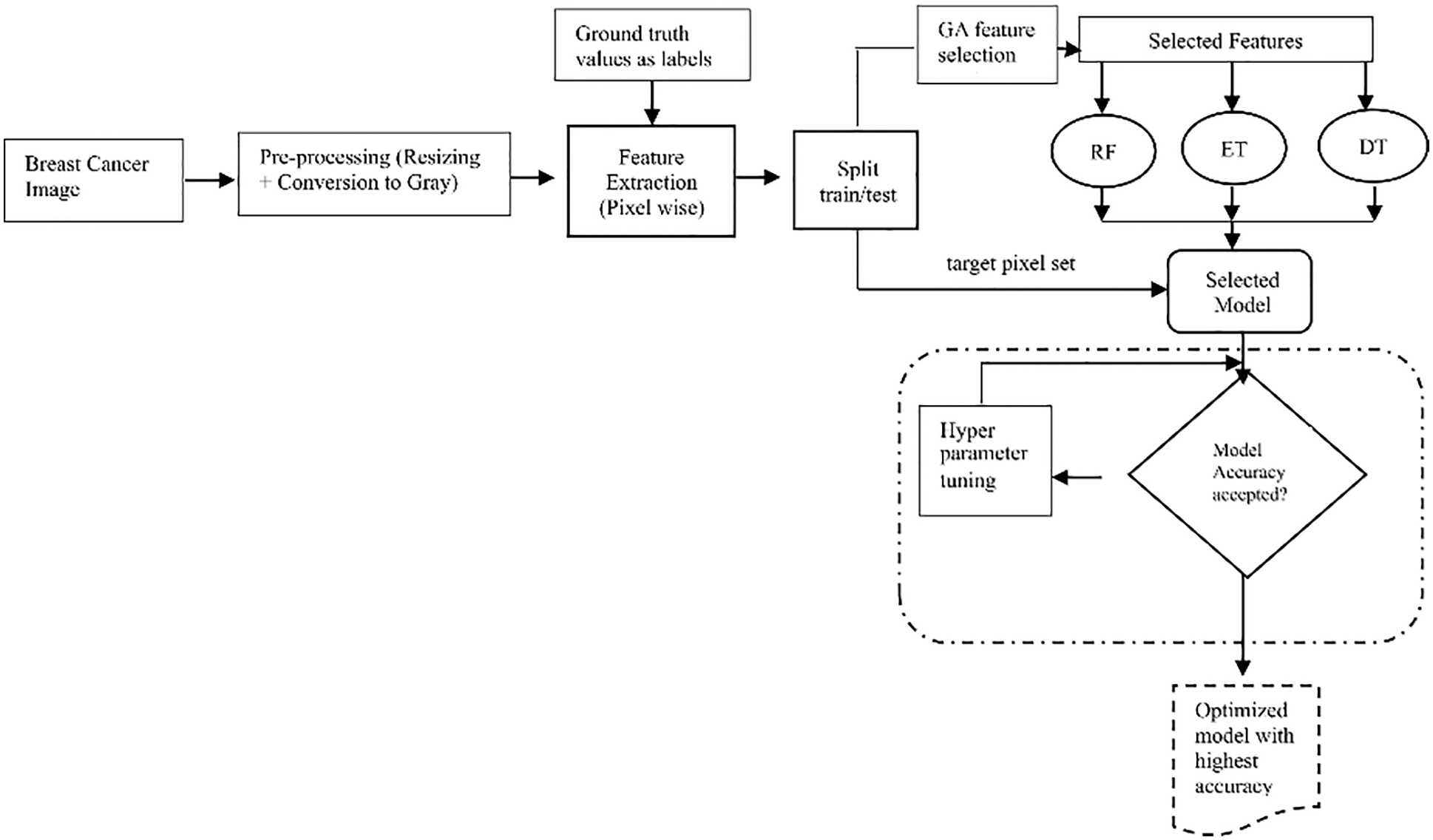
Figure 1: Process of hyperparameter optimization

3.4 Pre-Processing

Entire images of slides of tissues, of size 1360 × 1024, were converted into grayscale images of size 300 × 300. The image was resized for two reasons (a) to reduce the computational and memory-related costs, and (b) to render the image manageable.

3.5 Feature Extraction

3.5.1 Prewitt Edge Detection Filter

Digital filters are useful for image pre-processing tasks. A variety of filters have been used in the literature to extract the properties of images [25–29]. Prewitt operators are used to detecting edges along the x and y directions to yield masks Gx and Gy, respectively.

The Prewitt operator works on grayscale images and applies both masks one by one to determine the horizontal and vertical edges. Both edges are then combined to display the complete edges of the given image:

Gx(x,y)=[−101−101−101]×Im and(1)

Gy(x,y)=[−1−1−1000111]× Im(2)

Here Im is an image and the total magnitude in both directions can be calculated as

G=Gx2+Gxy2(3)

A higher value of G represents better edge detection. The direction (D) can be also determined as D∈{Gx,Gy}

3.5.2 Gaussian Filter

Gaussian blurring is a method of image denoising that is commonly used for image pre-processing. The Gaussian operator for a 2D distribution is as follows:

G(x,y)=12πσ2e(−x2+y2σ2)(4)

The value of sigma is important as it determines the width of the kernel image to be blurred. Higher values blur images over a larger area and lower values are used to limit this blurring area.

3.5.3 Gabor Filter

The Gabor filter acts as a local bandpass filter to extract spatial and edge-related features. It is constructed by using a Gaussian function in combination with a sinusoidal input. The filter can be expressed using parameters revised as eq (5) made more generalized, where θ represents the orientation of the filter, the sinusoidal radial frequency is W, and σx,σyare the standard deviations  Different Gabor filters can be constructed by changing the values of the parameters. Parameter settings are crucial for identifying the patterns.

G(x,y)=12πσxσyexp⁡(−12[xk2σx2+yk2σy2]).exp⁡[i(2πWxk+Ψ)](5)

wherexk=xcosθ+ysinθ

andyk=ycosθ−xsinθ

Ψ represents the phase shift as π2,π4….

3.5.4 Median Filter

The median filter is a non-linear digital filter that is commonly used to de-noise images. The median operation uses the median value of the pixels surrounding the pixel of interest. All pixel values are arranged and their median value is then selected as the value of the central pixel. Fig. 2 illustrates this process.

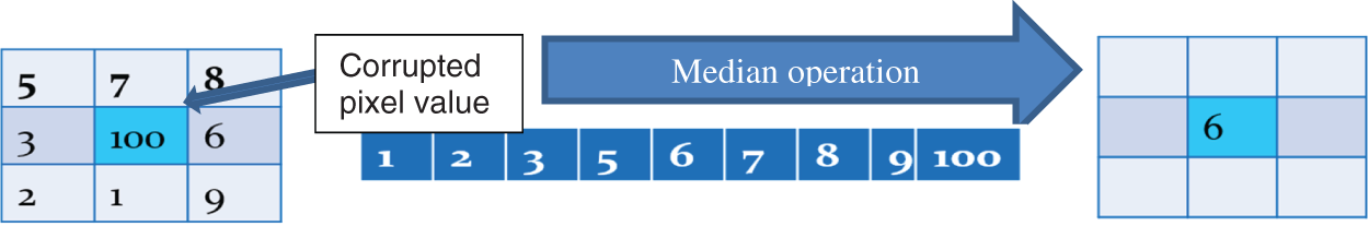
Figure 2: The median filter

3.6 GA-Based Feature Selection

This study uses the genetic algorithm (GA) to control the problem of dimensionality. The GA algorithm can search for the optimum value based on the survival-of-the-fittest theory. Genetic operators include selection, crossover, and mutation. These operators are applied to chromosomes (solutions) to optimize their fitness values. Chromosomes collections of genes as shown in Fig. 3a, where each gene represents a feature. For example, chromosome C = {gene1, gene2, …, genen} represents different intensities obtained from different combinations of filters.

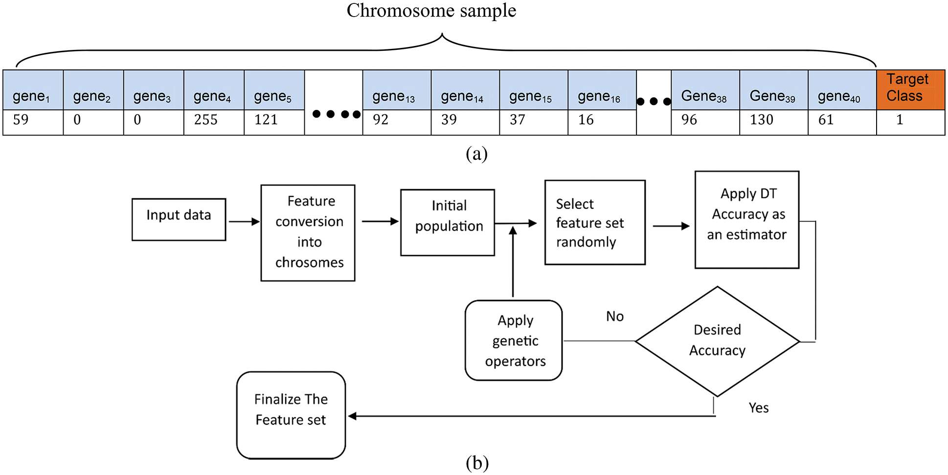
Figure 3: (a) Illustration of a sample chromosome. (b) Step-by-step process of GA-based feature selection

In the feature selection, “0” indicates the absence of a particular feature in the chromosome and “1” represents its presence. The initial population size, number of generations (iterations), crossover points, crossover probability, mutation probabilities, and techniques of chromosome selection are major considerations in this vein. The process of genetic programming is shown in Fig. 3b.

3.7 Principal Component Analysis (PCA)

The principal component analysis is a popular approach for dimension reduction in which an original set of attributes is orthogonally transformed into a new set of attributes. The relationship between the attribute sets (x, y) can be analyzed by a covariance matrix. Eigenvalues and eigenvectors are the fundamental measures used to determine the relevant components. The highest eigenvector with the maximum eigenvalue represents the first component, and the other components are calculated in decreasing order of value:

Covx,y=1n−1∑i=0n(xi−xm)(yi--ym)(6)

where, I = 0, 1, …., n, and xi is the value of the ith attribute and xmis the mean of the attribute values. yi and ym are the ith and the mean values of the second attribute set, respectively, and are used to calculate values of the eigenvector (e). I refer to an identity matrix, and λ represents the eigenvalues and eigenvectors obtained using Ae=λe. The complete eigenvectors corresponding to the eigenvalues can be found using Eq. (7). A is a covariance matrix:

(A−λiI)ei=0(7)

3.8 Supervised Classifiers

Machine learning algorithms are used to identify the important characteristics in a given dataset for predictive analysis or classification. This kind of identification is based on such attributes as the number of dimensions and the location of each data point. Medical images captured by advanced medical equipment provide a greater number and variety of features than images obtained by using traditional systems.

Fig. 4 shows the process of classifying each pixel of a given image into two essential categories. i.e., normal and cancerous.

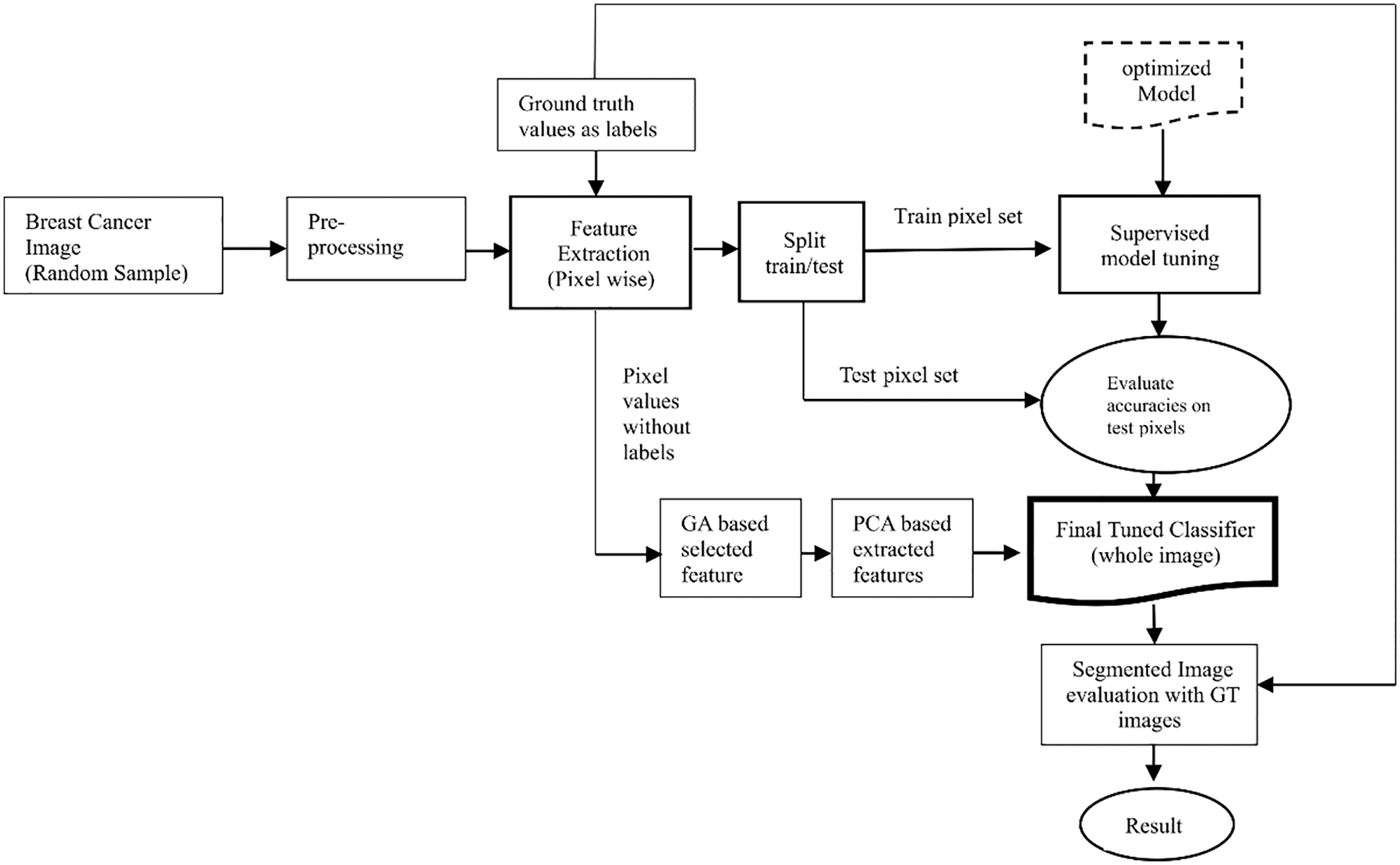
Figure 4: Pixel-level classification

The major steps are as follows: A random image is selected for classification. Features are extracted using a set of filters, and target values are assigned. Then the extracted dataset is split into training and testing subsets. Both subsets are submitted to the selected model. Training subset is useful to train the model for predicting each pixel value, whereas test subset result directs to tune and evaluate the model for better accuracy.

The final step consists of optimization using the genetic algorithm (GA) and principal component analysis (PCA). First, the GA selects the most discriminant and important feature set, which is processed by PCA to be limited to 12 components. Next, the tuned and aligned models are provided with the final components without their target values. The predicted values are then compared with the respective ground-truth values.

3.8.1 Random Forest (RF)

The RF classifier uses multiple decision trees to generate different sets of samples and calculates their average accuracy. Bootstrapping is carried out and random features are selected to this end, and the final decisions are taken according to the maximum voting principle. Such averaging is useful for handling the problem of model overfitting.

3.8.2 Decision Tree (DT)

The decision tree is used to evaluate data points on pre-specified, multiple “if-else” conditions. The end nodes contain a class of all possible classes.

3.8.3 Extra Tree (ET)

This classifier is similar to the random forest and applies multiple decision trees. In the extra tree classifier, all points are supplied to the tree, whereas subsamples are supplied in the RF.

3.9 Model Performance

3.9.1 Accuracy

True positive (TP) = number of positive samples correctly predicted.

False-negative (FN) = number of positive samples incorrectly predicted.

False-positive (FP) = number of negative samples incorrectly predicted as positive.

True negative (TN) = number of negative samples correctly predicted.

Accuracy (overall): the ratio of all correctly classified cases to the total number of cases. It is defined as

=(TP+TN)/(TP+FP+TN+FN)(8)

3.9.2 Image Quality Assessment

The predicted images are assessed using two image quality measures (a) Universal image quality index (UIQI) and Structural similarity index (SSI) [30,31]. Both quality measures have been discussed in Sections 4.4.1 and 4.4.2 respectively.

4  Experiments and Results

4.1 Datasets

We used the breast cancer histopathological annotation and diagnosis dataset (BreCaHAD). It is a collection of open-source, benchmark histopathological images of patients with breast cancer [32]. All images were obtained from case studies on surgical pathology. The slides were developed by H&E staining and the images were annotated. All images were available in eight-bit RGB color and had a size of 1360 × 1024 pixels. All biopsy images were classified into six malignant classes—mitosis, apoptosis, tumor nuclei, tubule, and non-tubule. Various settings were used to gather the histological structures with distinct boundaries to weakly define the histological structures. The dataset is available at https://doi.org/10.6084/m9.fgshare.7379186.

Another dataset consisting of ultrasound images was used. These images were classified as benign, malignant, or normal. The ground-truth values of each image are also provided in this open dataset, which can be accessed at the following link: Breast Ultrasound Images Dataset | Kaggle [33]. The dataset contained 600 images of patients with breast cancer, aged 25 to 75 years. All images had a size of 500 × 500 pixels in png format. The dataset also contained ground-truth images.

4.2 Experimental Setup

All experimental work was carried out by using the Google Colab cloud platform on the Tesla P100-PCIE GPU. Various Scikit learn and other packages were installed as required. The scripting language was Python 3.5 and the seed value was set to 42.

4.3 Model Selection and Optimization

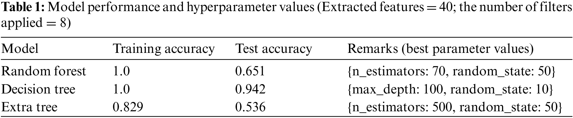
Tab. 1 represents the optimized hyperparameter values used for model learning. The model was trained and tested using all the extracted features, a total of 40, through different combinations and configurations of eight filters.

Tab. 2 shows the features extracted as well as the training and testing accuracies of the models considered. It shows that the DT provided the highest accuracy.

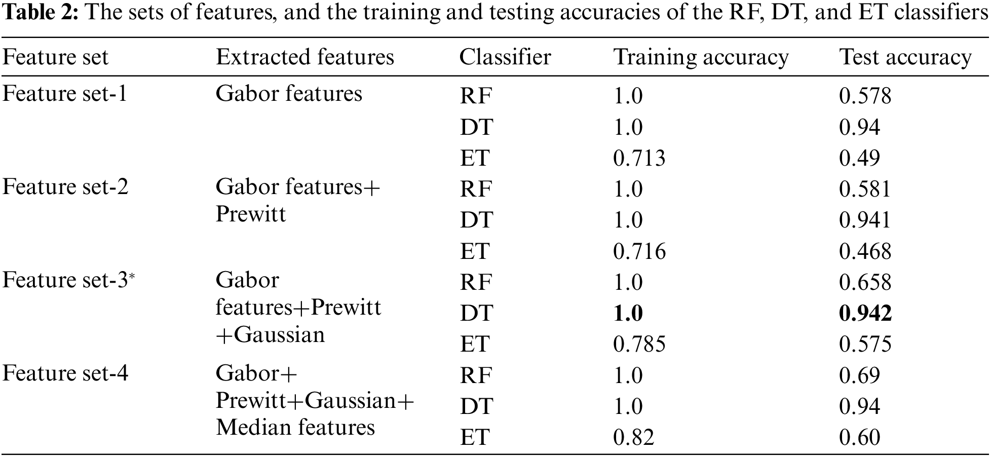
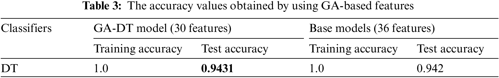
Tab. 2 shows that feature set-3 provided an accuracy of 0.942 by using only 36 features with the decision tree classifier. Feature set-3 was then supplied to the genetic algorithm for feature selection and reduction, and yielded only 30 prominent features. The pixel value of the original image has also been extracted as one of the features. The values of the GA operator were set as follows: population = 10, crossover probability = 0.5, mutation probability = 0.2, generation = 5, and tournament size = 3. The population and the number of generated values were reduced to minimize the computational cost. A lower probability of mutation was better for avoiding the local minimum. The reduced feature set obtained by the GA operator was fed to all three classifiers. The 30 features thus selected increased the testing accuracy by 0.1% (from 0.942 to 0.943). The accuracies of all classifiers are shown in Tab. 3.

When classifying the images, the population was set to 50 and the number of generations to 20 to ensure robust performance. The seed value was set to 42 to ensure that the results could be reproduced, and the components of PCA were limited to 12. This yielded a range of variance of 0.9999 to 1.0.

4.4 Strategy for Image Evaluation

To evaluate the images, an unlabeled image was first supplied to build the model (GA-PCA-DT) and the output of the model (predicted image) was compared with the respective ground-truth (labeled) image. The markers or labels of the predicted and the ground-truth images were then noted. The relevant steps are shown in Fig. 5.

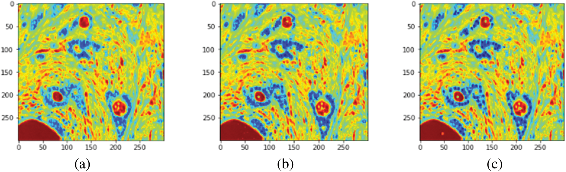
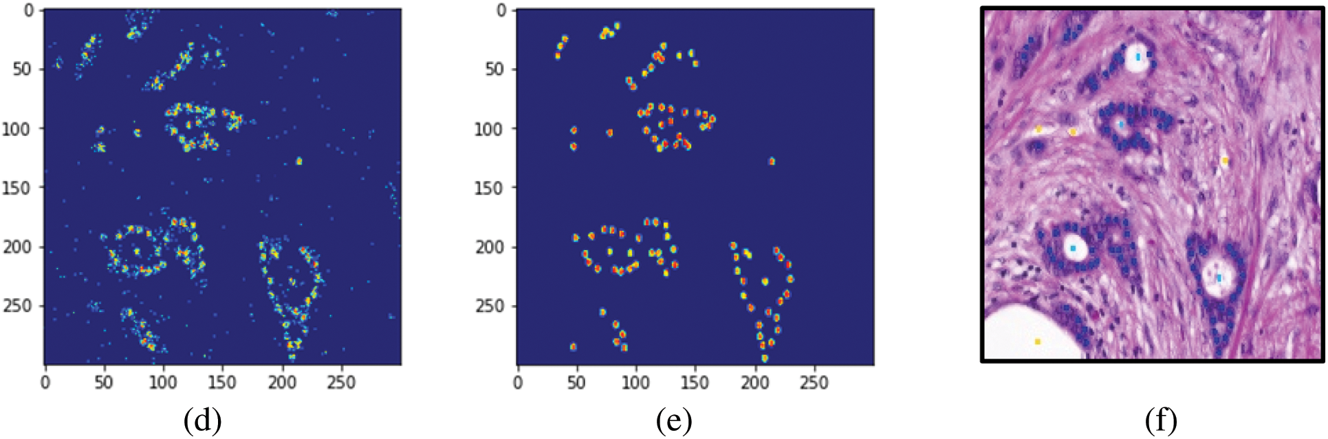
Figure 5: Processing histopathology images. (a) Resized original image (300 × 300). (b) The image was generated using the proposed GA-DT model. (c) The ground-truth image. (d) Labels assigned by the GA-DT model (e) Labels marked in the ground-truth image. (f) Original annotated image (in RGB)

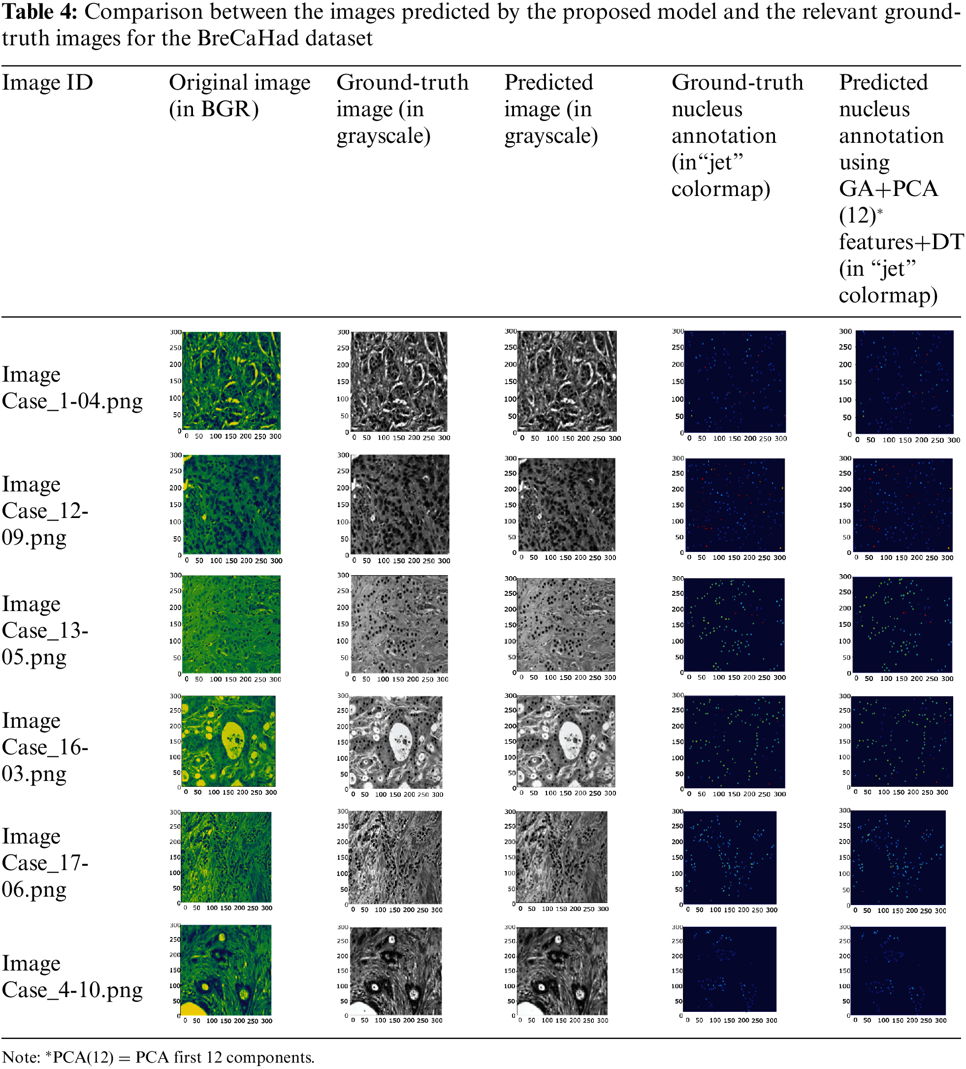
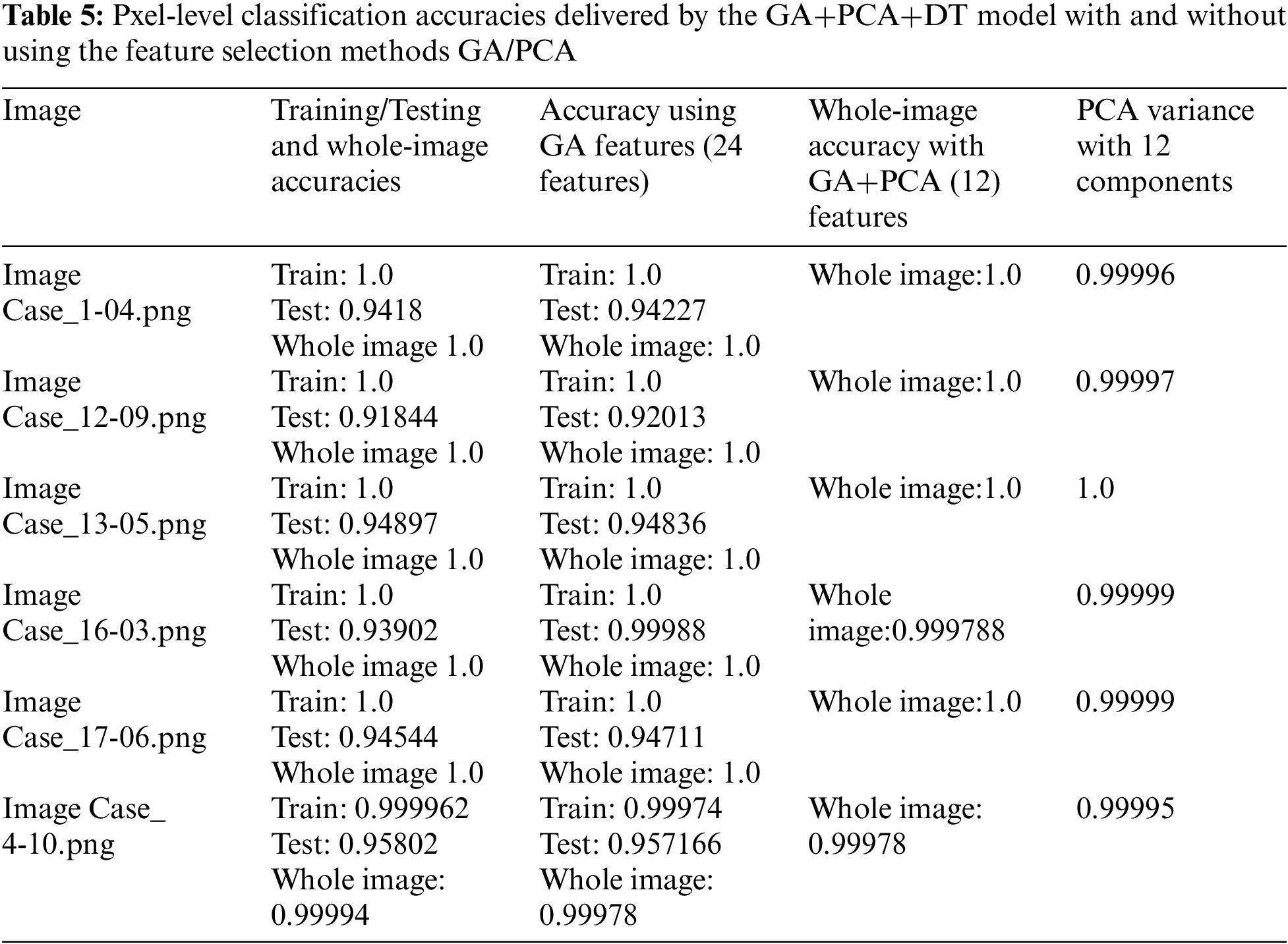
To check the robustness of the model, one image from each malignant class was randomly selected and supplied to it for label prediction. Tab. 4 lists the images predicted by the GA-PCA-DT model and the corresponding ground-truth images. Tab. 5 shows the pixel-level accuracies.

4.4.1 Graphical Illustration of UIQI

A simplified image quality measure, UIQI, has been proposed by Wang and Bovik. UIQI evaluates the quality of the test image over the referenced image by finding, loss in correlation, distortions in luminance and distortions in contrast. For example, suppose, Im and Ir are two images. Then UIQI value will be the product of all the above three components mathematically expressed as given in the reference [30]:

UIQI(Im,Ir)=σImIrσIrσIm.2.Im¯Ir¯,(Im¯)2+(Ir¯)2.2.σIrσImσIr2+σIm2(9)

UIQI has been employed to evaluate how the predicted images corresponded to the ground-truth images, as shown in Fig. 6.

Figure 6: UIQI scores of the predicted images

4.4.2 Graphical Comparison Based on SSI

An extension of the UIQI, structural similarity (SSI), was also proposed by Wang et al. [30,31]. The SSI is commonly used in videos and still images. It evaluates the degradation in image quality caused by pre-processing or losses in transmission. It uses two images to this end, i.e., the original and the processed image.

The SSI examines the similarity between the original and the processed image. It has a value between zero and one, where zero indicates that the images are completely dissimilar, and one indicates that they are identical. The SSI measure assumes that the human eye gathers image information through three channels, luminance, contrast, and structure present in the images. Therefore, SSI uses measurement functions for luminance (L), contrast (C), and structure (S). These functions are combined to calculate the final SSI value as represented in Eq. (10). Suppose Im and Ir are two images. To compare their image quality measure, SSI can be expressed as follows.

SSI(Im,Ir)=f(L(Im,Ir).C(Im,Ir).S(Im,Ir))(10)

A score of 0.99 and above is considered representative of satisfactory similarity. The SSI scores of the randomly selected images are shown in Fig. 7.

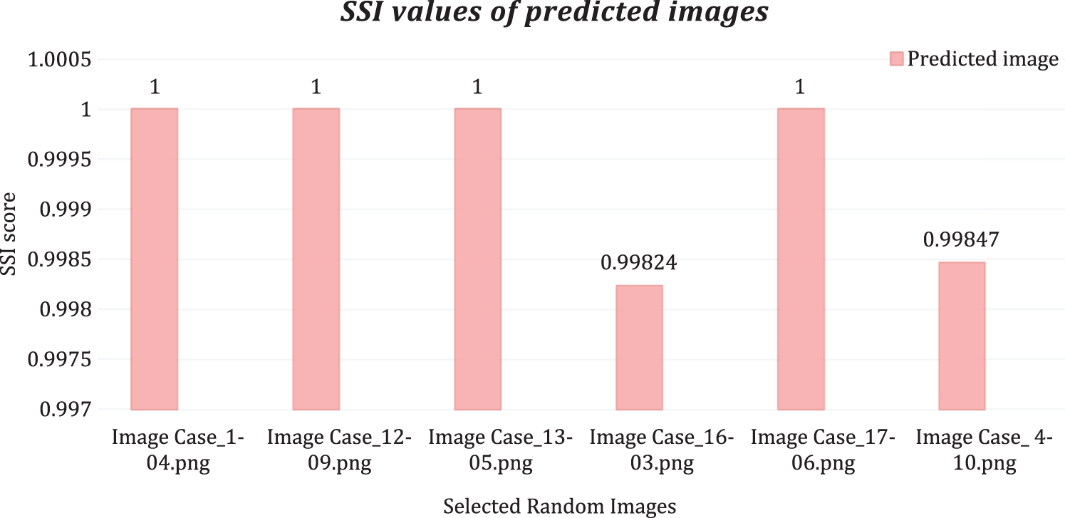
Figure 7: Structural similarity scores

Tab. 6 shows the classification-related performance of the proposed model based on the dataset of ultrasound images. Total extracted features are limited to 12 components using PCA and supplied to Decision Tree. The maximum accuracy pixel-level classification was obtained 1.0 for each test sample.

5  Conclusion and Future Work

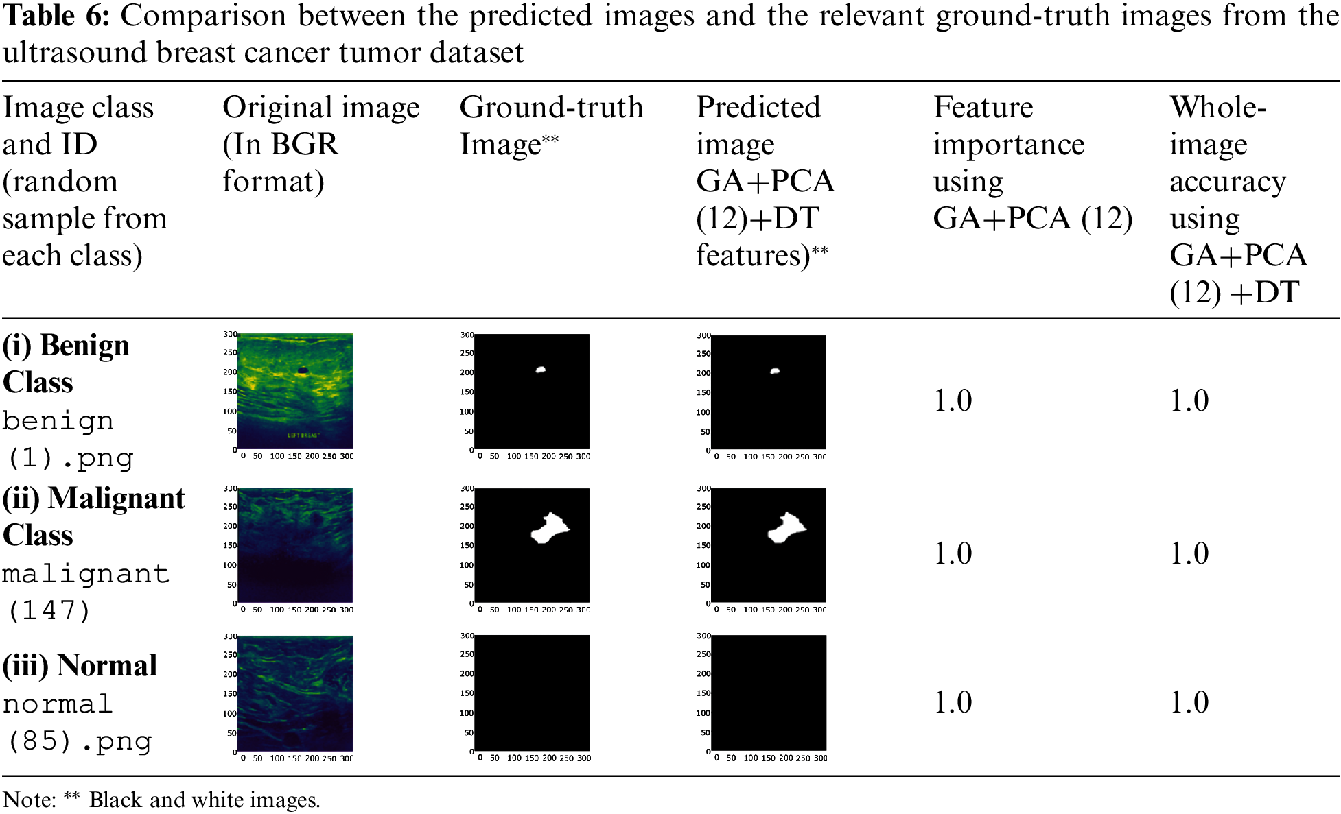
The proposed method successfully extracted prominent spatial features from the images through various filters, reduced feature set size by implementing GA and PCA in the combination, and accurately classified all pixels of chosen test images. The RF, DT, and extra tree models were built, and their hyperparameters were optimized based on the training and testing sets. The training accuracies of the GA-based method (without PCA) was 1.0, and testing accuracies ranged from 0.92 to 0.99 for the histopathology dataset. In the ultrasound image dataset, the model yielded training accuracies of 1.0 and testing accuracies from 0.9327 to 1.0. The final proposed model, GA-PCA-DT, was tested on images selected from each class. The proposed model has produced whole image classification accuracy between 0.9997 and 1.0. Furthermore, the predicted image (all pixels values) compared with respective ground-truth values generated UIQI scores in the range of 0.9999 to 1.0 and SSI scores in the range of 0.99824 to 1.0 for the test images, chosen randomly from every class of both datasets.

Breast cancer detection and annotation is a tedious and time-consuming task for every healthcare expert. The proposed model is simple, accurate, fast, and inexpensive, and thus can help classify whole image pixels into binary classes i.e., “disease” and “non-disease”. We believe that healthcare expert’s interventions are necessary for every medical examination and such automatic models can only assist experts at the primary level in expediting breast cancer detection, especially in the large populations or remote areas where healthcare facility is not sufficient.

The results reported here are excellent but slightly overfitted. The likely reasons for this are (a) a large number of target classes and (b) the consideration of exceptional pixel values as an additional class. The problem of overfitting can be solved by increasing the population size, further fine-tuning the model, and using regularization methods.

In future work, attention can be drawn to the use of more ML models, filters, and the employment of feature reduction techniques. In addition, different image quality measures can be explored to determine better evaluation. In this study, the images were resized to lower dimensions. Future studies can consider operations on the original images (i.e., 1360 × 1024), and RGB (i.e., red, green, blue) channels should be used instead of grayscale values.

The authors thank the following dataset contributors:

(a)   We thank Aksac et al. for providing a histopathological annotated dataset for breast cancer diagnosis for academic and research purposes, available at https://doi.org/10.6084/m9.figshare.7379186 (last accessed 31.01.22).

(b)   We also used ultrasound images for breast cancer diagnosis from the Breast Ultrasound Images Dataset | Kaggle.

Funding Statement: The authors received no funding for this study.

Conflicts of Interest: The authors declare that they have no conflicts of interest to report regarding the publication of this study.

References

1. R. L. Siegel, K. D. Miller, H. E. Fuchs and A. Jemal, “Cancer statistics,” CA: A Cancer Journal for Clinicians, vol. 71, no. 1, pp. 7–33, 2021. [Google Scholar]
2. M. M. Sunilkumar, C. G. Finni, A. S. Lijimol and M. R. Rajagopal, “Health-related suffering and palliative care in breast cancer,” Current Breast Cancer Reports, vol. 13, no. 4, pp. 241–246, 2021. [Google Scholar]
3. R. Wazirali and R. Ahmed, “Hybrid feature extractions and CNN for enhanced periocular identification during COVID-19,” Computer Systems Science and Engineering, vol. 41, no. 1, pp. 305–320, 2022. [Google Scholar]
4. P. Filipczuk, B. Krawczyk and M. Woźniak, “Classifier ensemble for an effective cytological image analysis,” Pattern Recognition Letters, vol. 34, no. 14, pp. 1748–1757, 2013. [Google Scholar]
5. G. Reshma, C. A. Atroshi, V. K. Nassa, B. T. Geetha, G. Sunitha et al., “Deep learning-based skin lesion diagnosis model using dermoscopic images,” Intelligent Automation & Soft Computing, vol. 31, no. 1, pp. 621–634, 2022. [Google Scholar]
6. S. Mane and S. Shinde, “A method for melanoma skin cancer detection using dermoscopy images,” in 2018 Fourth Int. Conf. on Computing Communication Control and Automation (ICCUBEA), Pune, India, pp. 1–6, 2018. [Google Scholar]
7. A. B. Tosun, M. Kandemir, C. Sokmensuer and C. Gunduz-Demir, “Object-oriented texture analysis for the unsupervised segmentation of biopsy images for cancer detection,” Pattern Recognition, vol. 42, no. 6, pp. 1104–1112, 2009. [Google Scholar]
8. A. V. Alvarenga, W. C. A. Pereira, A. F. C. Infantosi and C. M. Azevedo, “Complexity curve and grey level co-occurrence matrix in the texture evaluation of breast tumor on ultrasound images: Texture evaluation of breast tumor on ultrasound images,” Medical Physics, vol. 34, no. 2, pp. 379–387, 2007. [Google Scholar]
9. M. Moradi, P. Abolmaesumi, D. R. Siemens, E. E. Sauerbrei, A. H. Boag et al., “Augmenting detection of prostate cancer in transrectal ultrasound images using SVM and RF time series,” IEEE Transactions on Biomedical Engineering, vol. 56, no. 9, pp. 2214–2224, 2009. [Google Scholar]
10. R. S. Xu, O. Michailovich and M. Salama, “Information tracking approach to segmentation of ultrasound imagery of the prostate,” IEEE Transactions on Ultrasonics, Ferroelectrics and Frequency Control, vol. 57, no. 8, pp. 1748–1761, 2010. [Google Scholar]
11. S. Karacavus, B. Yilmaz, A. Tasdemir, O. Kayaalti, E. Kaya et al., “Can laws be a potential PET image texture analysis approach for evaluation of tumor heterogeneity and histopathological characteristics in NSCLC?,” Journal of Digital Imaging, vol. 31, no. 2, pp. 210–223, 2018. [Google Scholar]
12. M. Wu, R. F. Fraser and C. W. Chen, “A novel algorithm for computer-assisted measurement of cervical length from transvaginal ultrasound images,” IEEE Transactions on Information Technology in Biomedicine, vol. 8, no. 3, pp. 333–342, 2004. [Google Scholar]
13. M. M. R. Krishnan, V. Venkatraghvan, U. R. Acharya, M. Pal, R. R. Paul et al., “Automated oral cancer identification using histopathological images: A hybrid feature extraction paradigm,” Micron, vol. 43, no. 2, pp. 352–364, 2012. [Google Scholar]
14. B. S. Garra, B. H. Krasner, S. C. Horii, S. Ascher, S. K. Mun et al., “Improving the distinction between benign and malignant breast lesions: The value of sonographic texture analysis,” Ultrasonic Imaging, vol. 15, no. 4, pp. 267–285, 1993. [Google Scholar]
15. O. S. Al-Kadi, “Texture measures combination for improved meningioma classification of histopathological images,” Pattern Recognition, vol. 43, no. 6, pp. 2043–2053, 2010. [Google Scholar]
16. W. Gomez, W. C. A. Pereira and A. F. C. Infantosi, “Analysis of co-occurrence texture statistics as a function of gray-level quantization for classifying breast ultrasound,” IEEE Transactions on Medical Imaging, vol. 31, no. 10, pp. 1889–1899, 2012. [Google Scholar]
17. Y. -L. Huang, K. -L. Wang and D. R. Chen, “Diagnosis of breast tumors with ultrasonic texture analysis using support vector machines,” Neural Computing and Applications, vol. 15, no. 2, pp. 164–169, 2006. [Google Scholar]
18. Y. -L. Huang, D. -R. Chen and Y. -K. Liu, “Breast cancer diagnosis using image retrieval for different ultrasonic systems,” in 2004 Int. Conf. on Image Processing. ICIP ’04, Singapore, vol. 5, pp. 2957–2960, 2004. [Google Scholar]
19. R. Rashmi, K. Prasad, C. B. K. Udupa and V. Shwetha, “A comparative evaluation of texture features for semantic segmentation of breast histopathological images,” IEEE Access, vol. 8, no. 1, pp. 64331–64346, 2020. [Google Scholar]
20. F. A. Spanhol, L. S. Oliveira, C. Petitjean and L. Heutte, “A dataset for breast cancer histopathological image classification,” IEEE Transactions on Biomedical Engineering, vol. 63, no. 7, pp. 1455–1462, 2016. [Google Scholar]
21. D. Kramer and F. Aghdasi, “Texture analysis techniques for the classification of microcalcifications in digitised mammograms,” in 1999 IEEE Africon. 5th Africon Conf. in Africa (Cat. No.99CH36342), Cape Town, South Africa, pp. 395–400, 1999. [Google Scholar]
22. H. Soltanian-Zadeh, S. Pourabdollah-Nezhad and F. Rafiee Rad, “Shape-based and texture-based feature extraction for classification of microcalcifications in mammograms,” in Proc. SPIE 4322, Medical Imaging 2001, San Diego, CA, pp. 301–310, 2001. [Google Scholar]
23. R. Kumar, R. Srivastava and S. Srivastava, “Microscopic biopsy image segmentation using hybrid color K-means approach,” International Journal of Computer Vision and Image Processing, vol. 7, no. 1, pp. 79–90, 2017. [Google Scholar]
24. A. Khanna, N. D. Londheand and S. Gupta, “Automatic lung segmentation and airway detection using adaptive morphological operations,” in Machine Intelligence and Signal Analysis, In: M. Tanveer, R. B. Pachori (eds.Vol. 748. Singapore: Springer, pp. 347–354, 2019. [Google Scholar]
25. X. Li and K. N. Plataniotis, “A complete color normalization approach to histopathology images using color cues computed from saturation-weighted statistics,” IEEE Transactions on Biomedical Engineering, vol. 62, no. 7, pp. 1862–1873, 2015. [Google Scholar]
26. P. -W. Huang and Y. -H. Lai, “Effective segmentation and classification for HCC biopsy images,” Pattern Recognition, vol. 43, no. 4, pp. 1550–1563, 2010. [Google Scholar]
27. Z. Wang and W. T. Ang, “Automatic dissection position selection for cleavage-stage embryo biopsy,” IEEE Transactions on Biomedical Engineering, vol. 63, no. 3, pp. 563–570, 2016. [Google Scholar]
28. R. Sarkar and S. T. Acton, “SDL: Saliency-based dictionary learning framework for image similarity,” IEEE Transactions on Image Processing, vol. 27, no. 2, pp. 749–763, 2018. [Google Scholar]
29. M. Sapkota, F. Liu, Y. Xie, H. Su, F. Xing et al., “AIIMDs: An integrated framework of automatic idiopathic inflammatory myopathy diagnosis for muscle,” IEEE Journal of Biomedical and Health Informatics, vol. 22, no. 3, pp. 942–954, 2018. [Google Scholar]
30. Z. Wang and A. C. Bovik, “A universal image quality index,” IEEE Signal Processing Letters, vol. 9, no. 3, pp. 81–84, 2002. [Google Scholar]
31. M. Oszust, “Full-reference image quality assessment with linear combination of genetically selected quality measures,” PLOS ONE, vol. 11, no. 6, pp. 1–17, 2016. [Google Scholar]
32. A. Aksac, D. J. Demetrick, T. Ozyer and R. Alhajj, “BreCaHAD: A dataset for breast cancer histopathological annotation and diagnosis,” BMC Research Notes, vol. 12, no. 82, pp. 1–3, 2019. [Google Scholar]
33. W. A. Dhabyani, M. Gomaa, H. Khaledand and A. Fahmy, “Dataset of breast ultrasound images,” Data in Brief, vol. 28, no. 1, pp. 104863, 2020. [Google Scholar]
Cite This Article
Copyright © 2023 The Author(s). Published by Tech Science Press.
This work is licensed under a Creative Commons Attribution 4.0 International License , which permits unrestricted use, distribution, and reproduction in any medium, provided the original work is properly cited.
Downloads
Citation Tools