Machine Learning-based Electric Load Forecasting for Peak Demand Control in Smart Grid

1  Introduction

As the population and industrializing are increasing, the corresponding energy demand is increasing year by year exponentially. Worldwide the energy demand is increasing at an alarming rate of 3%–5% every year for the half-decade. Most countries are dependent on fossil fuels for their energy demands across the world [1]. Climate change become a global problem today due to greenhouse emissions and by burning of fossil fuels for energy. The burning of fossil fuels is the major cause of air pollution and it leads to major health problems. Therefore, the use of low carbon energy souses like renewable energy is increasing in the power sector day by day to reduce CO2 emissions. This type of clean and affordable source of energy is important for climate change as well as it is required for fighting poverty also [2]. The energy consumption of India will also increase to 11% by 2040 of global energy demand as shown in Fig. 1. The renewable-energy become a significant player in the last decade in India to decrease the pollution level of the environment. Indian Government has introduced various initiatives for renewable energy expansion like the Rooftop Solar program, solar parks, providing huge subsidies for renewable energy installation, etc.

Figure 1: Expected energy consumption of India

But as renewable energy like wind and solar will increase in the grid, the stability of the grid will also affect due to its noncontinuous nature. Power systems face various technical issues like Power Quality Issues, Power and voltage fluctuations, Storage, Protection issues, and Islanding on increasing the renewable energy in the grid. So, it is required proper planning of power systems to maintain the power quality of a renewable-based grid. The prior forecasting of the electrical load can efficiently build a power system that could fulfil the unerupted power supply shown in Fig 2. It would be more efficient than the conventional power system designed based on vague assumptions [3,4].

Figure 2: The proposed plan for peak load control

Artificial-based forecasting techniques could help in the proper planning of transmission and distribution (T&D) facilities. Transmission and distribution buses are built to hold a certain capacity of voltage (V) and current (I). Using this load prediction technique, V&I can determine indirectly, and hence T&D buses operating capacity can be known. It helps in the correction of voltage, power factor, etc. which finally reduces losses [5].

The work of load prediction is to give an idea about the demand side so the supply side can be ready accordingly. This pre-preparation of the supply side can help exact load feeding. This helps in reducing losses by avoiding fluctuation in load on the demand and supply side. Most of the power plants in India are thermal power plants. The coal of high grade is imported and hence is to be efficiently used. Load prediction helps inefficient fuel management by determining load at a certain hour of the day before. Information and Communication Technology helps in a reliable grid formation and grid management. This is possible as the frequency fluctuation can be minimized using load prediction [6,7]. It leads to improved economics and manpower development. Load forecasting supports utilities to make significant decisions like purchasing and generating electric power and infrastructure development. Helps in accessing power system security. If the predicted load is not matching the actual load by a great margin in an accurate model implies electricity theft. A scheduling function can be formed well in advance that decides the most economic commitment of generating sources [8]. In most of the literature the concreate solution of peak demand load control techniques is not discussed. All the present techniques of peak load control have is own limitations. In this paper the machine learning techniques is used for forecasting of demand load 24 h before, so the demand load and peak load can control and managed properly. In this way the grid reliability and safety can be enhanced.

2  Machine Learning in Power System

There are two types of electrical load namely base load and peak load. The baseload is almost constant and the peak load is fluctuating in nature. The stability of the power grid may enhance by predicting the peak load using machine learning techniques. Therefore, the study is based on machine learning, and to better understand it existing methods are discussed based on the model used. There are two types of classes: Linear and non-linear. Linear models are simple models. It uses the method of least-square approximation to fit in the best line that would satisfactorily describe the data. The method of least-squares as stated earlier is a widely used linear class technique [9]. There can be a huge error at times if data points are sparsely spaced. To increase accuracy and minimize error non-linear models can be used. The electrical load has a lot of non-linearity, so this approach may not be best suited for this study. Non-linear models are complex, time-consuming, and require an ample number of computations. But the results produced are better compared to linear models. The two terminologies that would be mostly used in this study are the Prediction variable and the response variable. They require features or factors on which the response variable depends to train a model termed prediction variables. The response variable is the one whose value is to be predicted based on the prediction variable. Whenever there is non-linear dependence between prediction variables non-linear models are used. Examples of non-linear models are Support Vector Machines (SVMs), Gaussian process regression (GPR), etc. SVMs along with ant colony (AC) optimization proves to be an accurate technique for load prediction [10,11]. All the techniques linear, and non-linear are similar in their methodology. They just differ in the type of kernel used. Load prediction can be short-term, long term or medium-term based on the time of prediction and the time when data is trained. Prediction is a tricky task. The accurate prediction requires the accurate information and factors on which the prediction is going to depend. If one takes into account all the factors then the size of data increases moreover chances of over-fitting of data too. There must be optimal feature selection such that the features are not redundant. Load is predicted based on historical load data. Hence, a lot of historical load data of place is required for accurate load prediction [12]. Prediction techniques are classified as shown in the Fig. 3.

Figure 3: Classification of load forecasting techniques

In our study, the electric demand load will predict at a certain hour of the day depending on various prediction variables. This is a regression problem. Regression is predicting a variable termed a response variable based on the values of prediction variables and their relation with the response variable. Regression can be linear: there is one response variable and one prediction variable; Multiple: there is one response variable and many predictions variable; Multivariate: there are many response and prediction variables. This classification is based on various input and output variables. Based on the curve used for fitting it can either be linear regression or polynomial regression [13,14]. Choosing the best model is depend on the modelling and simulation results. There are various regression algorithms like SVMs, K-Nearest Neighbour (KNN), Neural networks, Artificial Neural Network (ANN), GPR, etc. Every algorithm has its merits and demerits one must analytically choose the best algorithm based on computation time, complexity, and hyperparameter requirement. Performance parameters are R-Square (RS)/Adjusted-R Square, Root Mean Square Error (RMSE)/Mean Square Error (MSE), and Mean Absolute Error (MAE) [15]. The data relating to all the above-mentioned factors are important to be obtained to get the desired accuracy. While collecting data, the noise gets into the system. This noise is to be filtered using statistical filters or mathematical computations. Large error-free data is required for an effective machine learning model. Moreover, data collected must be such that it has high and independent co-variance with the response variable and other prediction variables [16,17].

3  Electrical Load Datasets for Modeling

The data for modelling and simulation is taken from the 33 kV grid of Jajpur road, Orissa. The Jaipur Road 33 KV grid is a substation of Orissa Power Transmission Corporation Limited (OPTCL). OPTCL is the State Transmission Utility (STU) and functions as the State Load Dispatch. Here, Jajpur road 33 kV grid one-year data is taken for simulation. The data is recorded hourly wise so the total data is 8760 is used for simulation. The dataset contained 8760 rows along with 10 columns (9 prediction variables and 1 response variable) arranged hourly from January 1, 2018, to December 31, 2018. The January 2019 data (total 744 data) is kept for testing of the suitable model. The hourly electrical load data and temperature of the Jajpur of each month from January 1, 2018, to December 31, 2018 is shown in Fig. 4.

Figure 4: Monthly electrical load and temperature of Jajpur (Y axis-Temperature in °C & Electrical load in MW)

4  Data Synthesis and Preparation

The formulated data may have noises that can disturb the results, so it requires to be filtered. Moreover, the gathered data can be transformed into formats compatible with the software. Such transformation is needed to make noise-free to ensure all the random data was erased and the data was made smooth. Now, the target dataset is divided into training data, test data and validation data whose ratio is based on the availability of data for evaluation. One can either use hold-out validation or cross-validation. the study used 10-fold cross-validation (CV). In this technique one-tenth of the data is taken as validation data and the rest as training data. The tests are validated with a new dataset after trained of the proper model. The tested model check for various performance parameters that helps in choosing the best model out of all trained models [18]. This step is important as it gives an idea about the effectiveness model. If the results are not satisfactory then need to repeat the above-mentioned steps. The different algorithms chosen for study must contain different parameters on which they depend. To choose an optimal value of these parameters one has to do trial and error. Choose a wide range of values for this parameter and choose the one that reduces error and increases accuracy. Fine-tuning models can improve model performance. Hyper-parameters comprise several training steps, learning rate, initial values and many more. RMSE is the performance parameter and model with the least value of RMSE [19,20]. Once all the model has gone through the above-mentioned steps, they can be chosen as an appropriate model for predictions. The model is to be maintained and checked every short period for it to remain equally reliable and effective. All these steps are involved in getting effective results. These are general steps required in any machine learning problem. One may add or remove a few steps based on requirements. Heat maps and Pair plots are a great method to correlate the input of the data with the output [21,22].

The following correlation is showing in Fig. 5 graphical representation of a correlation matrix representing the correlation between different variables. It shows the importance of different input variables based on their priority. Therefore, the least important factors or input variables may neglect to minimize the complexity of the model. The Fig. 6 shows correlation maps discuses about how two variables are linearly correlated. In any forecasting techniques, correlation between features and the target variable try to maximize. Because, higher the correlation, more useful that feature in order to predict the target variable [23]. It means heatmaps and pair plot correlation are a quick way to look at one to one relationship between input and output in a forecasting technique. For small number of features, might be able to look at multi-variable linear dependencies. Here the demand load is correlated with pressure, cloud, humidity, rain, gust, wind, feels of temperature and temperature. The greater value in heatmap is showing greater the relationship of input and output. Similarly, the more linear relationship graph of pair plot correlation has more dependency of input on output. Based on the following correlation map it is concluded that the temperature and feel of temperature is the most important factor for electrical load forecasting [24].

Figure 5: Correlation heatmap

Figure 6: Pair plot correlation

5  Modelling of Data for Simulation

In the model, Gaussian process regression (GPR) is giving the best result for the electrical load data of the Jajpur, Odisha India. Here, the maximum number of values predicted values is matched with the true value. The error is also less compared to the other models. GPR models are kernel-based non-parametric probabilistic models. Each electric data can be represented as following equation in the different machine learning models [25].

Suppose the input training dataset is {(xi,yi); wherei=1,2,…,n}(i)

The equation followed by the linear regression model is y=xTβ+ε where ε∼N(0,σ2)(ii)

where xi ∈ ℝd and yi ∈ ℝ, taken from an electrical dataset distribution and σ2 and β are the error variance and coefficients respectively.

The joint distribution of this GPR is expressed as P (f | X) ∼ N (f | 0, K (X, X)). This expression is near to a linear regression model. The K(X, X) for this expression may be denoted as

K(X,X)=(K(x1,x1)K(x1,x2)⋯K(x1,xn)K(x2,x1)K(x2,x2)⋯K(x2,xn)⋮⋮⋮⋮K(xn,x1)K(xn,x2)⋯K(xn,xn))(iii)

Then the Rational Quadric GPR Model will k(xi,xj|θ)=σf2(1+r22ασl2),(iv)

where θ is the maximum estimate and σf standard deviation of the signal. α non-negative parameter of the covariance and

r=(xi−xj)T(xi−xj)(v)

The input training data of Eq. (i) can be represents in the Matern 5/2 GPR. It is generate Fourier transforms of radial basis function. It does not applicable for high dimensional spaces related problems. So, the matern 5/2 GPR algorithm can be represent as follows.

Then,The Matern 5/2GPR Model will as k(Xi,Xj|θ)=σf2(1+3rσl)exp(−3rσl);(vi)

The Squared Exponential GPR: It is same as Exponential GPR except that the Euclidean distance is squared. This model can be handle large data sets without producing measurable errors. The algorithm of the squared exponential GPR can be represent for the same data set (i) as follow

Similarly, The Square Exponential GPR Model becomes:

k(xi,xj|θ)=σf2exp[−12(xi−xj)T(xi−xj)σl2](vii)

Finally,the Exponential GPR Model becomes:k(Xi,Xj|θ)=σf2exp(−rσl)(viii)

The Eqs. (ii) and (v) is used for finding the y and r in above equation.

The above Figs. 7 and 8 showing the simulation result of electric data by Fine Gaussian GPR and Support Vector (SVM) Machine methods. Since GPR and SVM is showing best result in all the simulation. Therefore, it is taken for consideration. The graph is showing the actual and predicted electrical data. The most of the data is overlapping. Ideally, the actual and predicted data should overlap accurately. In the other graph the true response and predicted response should near the straight line. As the points will near the straight line the result show good result. This can be minimised by increasing the quantity and quality of the data.

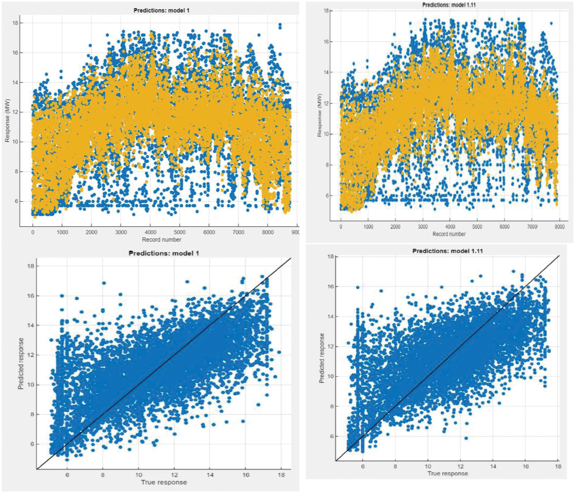
Figure 7: Fine gaussian and support vector machine

Figure 8: Data modelling by GPR

6  Results and Discussion

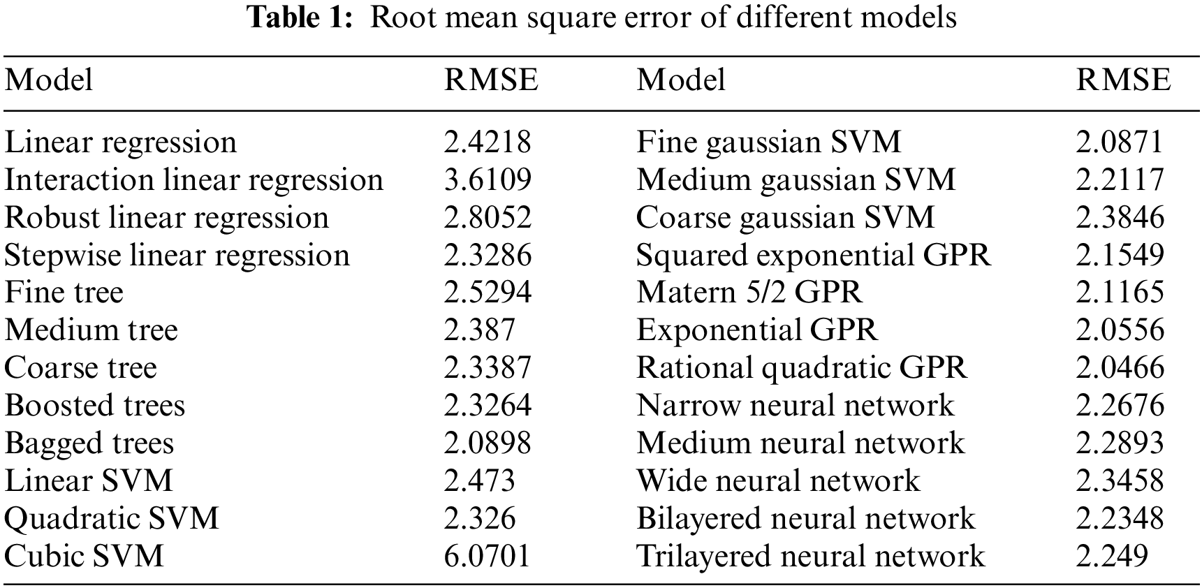
The study is based on machine learning using regression. therefore, the above-mentioned steps were followed. Once the data was ready it was to be trained. Data were divided into training data and test/validation data. A total of 12 months (January 2018 to December 2018) of an electric load of the Jajpur grid is taken for training. One month load data of January 2019 and next month’s February 2019 dataset is taken for validation and testing respectively. All the data is collected hourly wise. Training data was trained using algorithms like Support Vector Machine (SVM), Tree, Gaussian Process Regression (GPR), Wide Neural Network etc. The results obtained in the form of RMSE as performance parameters of a different model are shown in Tab. 1 below. RMSE is the performance parameter, the lower the value of RMSE better is the performance of the model.

GPR had the least value of RMSE and hence can be treated as the best model based on the performance parameter chosen as shown in the Fig. 9. The result on visualization seems less accurate for both the algorithms but their RMSEs are amongst the lowest. Such a plot was obtained for the best model i.e., Gaussian Process Regression (GPR) shown below. The test data was chosen to verify the model and the results produced are shown below. The plots on top are the response plots for both the models and the plots on the bottom show how distributed are the values from the true values.

Figure 9: RSME chart

The plot shown in the Figs. 10 and 11 is presenting the actual and predicted electric load. The actual and predicted electrical demand load are almost overlap each other in the both the above diagram, showing the accuracy of the algorithm. There are places where the graph is not smoothly followed which can be corrected using increased quantity and quality of the dataset. In the present study, the electrical load data from January 1, 2018 to January 31, 2019 is used for modelling. It means the total 13 months data is used for is used for study where the data is available in hourly of each day. The 12 months data is used for the modelling and one month data is used for verifying the model. The actual electricity demand and predicted electricity demand of the month January 2019 is shown in blue and red in Fig. 10 and black and red respectively in the Fig. 11. The Figs. 10 and 11 are almost overlapping to each other. It means that actual data and predicted is almost same which validate the model.

Figure 10: Actual value vs. predicted value

Figure 11: Actual vs. predicted value (C-Actual load and D-Predicted load)

7  Conclusion

This study is based on Regression type machine learning. The best model for load prediction is Rational Quadratic Gaussian Process Regression on the basis of root mean square error for the present jajpur data. Because, The RMSE Rational Quadratic Gaussian Process Regression is 2.0466 which is minimum compare to the other mathematical models. But, the computation time for GPR was the highest as it was the most complex algorithm among all of the models trained. SVM was the second-best algorithm whose RMSE value is 2.0871, but the computation time was very less of SVM. So, there is a trade between computation time and RMSE. Also, SVM is a simple algorithm. So, it is based on the researcher choosing the algorithm according to the requirement of the dataset. The algorithm produced satisfactory results but could be improved to produce better results. The data train was made using only one year of load data. This data was very less but was enough for analysis point of view. This small amount of data can undergo underfitting or overfitting of the model. The load was predicted so need a different prediction variable. The more the non-redundant prediction variables better would be the results produced. In our case, limited prediction variables were chosen and hence, the result could be made better by including the left-out factors. Features selected were only ac-counting weather conditions. Factors like time factor, population, customer class, etc. could also be included. The data had 8760 rows accounting for one-year load data. Therefore, getting data for the past few more years can lead to improved results. Hyper-parameter tuning is not implemented in this study which may improve results. In the present study, the electrical load data from January 1, 2018 to January 31, 2019 is used for modelling. It means the total 13 months data is used for is used for study where the data is available in hourly of each day. The 12 months data is used for the modelling and one month data is used for verifying the model. The actual electricity demand and predicted electricity demand of the month January 2019 is shown in black and red respectively in the Fig. 11. The actual and predicted graph is almost overlapping to each other in the Fig. 11. It means that actual data and predicted load are almost same. This is showing validation of the models. The peak load management become more easier if the demand load can predict one day before. The result clearly showing that the electric demand load can be forecast exactly and accurately using the machine learning techniques discussed in the paper.

Funding Statement: The authors received no specific funding for this study.

Conflicts of Interest: The authors declare that they have no conflicts of interest to report regarding the present study.

References

1. M. J. C. Espinoza, J. U. Suykens, R. U. Belmans and B. U. J. De Moor, “Electric load forecasting-using kernel-based modelling for nonlinear system identification,” IEEE Control Systems Magazine, vol. 27, no. 5, pp. 43–57, 2007. [Google Scholar]
2. A. Abessi, V. Vahidinasab and M. S. Ghazizadeh, “Centralized support distributed voltage control by using end-users as reactive power support,” IEEE Transactions on Smart Grid, vol. 7, no. 1, pp. 178–188, 2016. [Google Scholar]
3. K. Mahmud, J. Ravishankar, M. J. Hossain and Z. Y. Dong, “The impact of prediction errors in the domestic peak power demand management,” IEEE Transactions on Industrial Informatics, vol. 16, no. 7, pp. 4567–4579, 2020. [Google Scholar]
4. N. Huang, W. Wang, S. Wang, J. Wang, G. Cai et al., “Incorporating load fluctuation in feature importance profile clustering for day-ahead aggregated residential load forecasting,” IEEE Access, vol. 8, pp. 25198–25209, 2020. [Google Scholar]
5. A. Ahmad, N. Javaid, A. Mateen, M. Awais and Z. Khan, “Short-term load forecasting in smart grids: An intelligent modular approach,” Energies, vol. 12, no. 1, pp. 164, 2019. [Google Scholar]
6. M. Jawad, M. Nadeem, S. Shim, I. Khan, A. Shaheen et al., “Machine learning-based cost-effective electricity load forecasting model using correlated meteorological parameters,” IEEE Access, vol. 8, pp. 146847–146864, 2020. [Google Scholar]
7. N. Zhang, J. Xiong, J. Zhong and K. Leatham, “Gaussian process regression method for classification of high-dimensional data with limited samples,” in Proc. of Eighth Int. Conf. on Information Science and Technology, Granada, Cordoba, and Seville, Spain, pp. 358–363, 2018. [Google Scholar]
8. A. Baliyan, K. Gaurav and S. Mishra, “A review of short-term load forecasting using artificial neural network models,” Procedia Computer Science, vol. 48, pp. 121–125, 2015. [Google Scholar]
9. B. Nepal, M. Yamaha, A. Yokoe and T. Yamaji, “Electricity load forecasting using clustering and ARIMA model for energy management in buildings,” Japan Architectural Review, vol. 3, no. 1, pp. 6276, 2020. [Google Scholar]
10. X. Wang, W. Lee, H. Huang, R. Szabados, D. Y. Wang et al., “Factors that impact the accuracy of clustering-based load forecasting,” IEEE Transactions on Industry Applications, vol. 52, no. 5, pp. 3625–3630, 2016. [Google Scholar]
11. J. Luo, T. Hong and S. Fang, “Benchmarking robustness of load forecasting models under data integrity attacks,” International Journal of Forecasting, vol. 34, pp. 89–104, 2018. [Google Scholar]
12. S. Motepe, A. Hasan and R. Stopforth, “Improving load forecasting process for a power distribution network using hybrid AI and deep learning algorithms,” IEEE Access, vol. 7, pp. 82584–82598, 2019. [Google Scholar]
13. S. Habib, S. Alyahya, A. Ahmed, M. Islam, S. Khan et al., “X-ray image-based COVID-19 patient detection using machine learning-based techniques,” Computer Systems Science and Engineering, vol. 43, no. 2, pp. 671–682, 2022. [Google Scholar]
14. S. Prabu, B. Thiyaneswaran, M. Sujatha, C. Nalini and S. Rajkumar, “Grid search for predicting coronary heart disease by tuning hyperparameters,” Computer Systems Science and Engineering, vol. 43, no. 2, pp. 737–749, 2022. [Google Scholar]
15. X. Guo, Y. Zhang, S. Lu and Z. Lu, “A survey on machine learning in COVID-19 diagnosis,” CMES-Computer Modeling in Engineering & Sciences, vol. 130, no. 1, pp. 23–71, 2022. [Google Scholar]
16. A. Jozi, T. Pinto, I. Praça and Z. Vale, “Decision support application for energy consumption forecasting,” Appl. Sci., vol. 9, pp. 699, 2019. [Google Scholar]
17. Y. Wang, Z. Liao, S. Shi, Z. Wang and L. H. Poh, “Data-driven structural design optimization for petal-shaped auxetics using isogeometric analysis,” Computer Modeling in Engineering & Sciences, vol. 122, no. 2, pp. 433–458, 2020. [Google Scholar]
18. R. Cheng, Y. Xiaomeng and L. Chen, “Machine learning enhanced boundary element method: Prediction of Gaussian quadrature points,” Computer Modeling in Engineering & Sciences, vol. 131, no. 1, pp. 445–464, 2022. [Google Scholar]
19. A. H. Seh, J. F. Al-Amri, A. F. Subahi, A. Agrawal, N. Pathak et al., “An analysis of integrating machine learning in healthcare for ensuring confidentiality of the electronic records,” Computer Modeling in Engineering & Sciences, vol. 130, no. 3, pp. 1387–1422, 2022. [Google Scholar]
20. B. Sakthivel, K. Jayaram, N. M. Devarajan, S. M. Basha and S. Rajapriya, “Machine learning-based pruning technique for low power approximate computing,” Computer Systems Science and Engineering, vol. 42, no. 1, pp. 397–406, 2022. [Google Scholar]
21. R. Iqbal, H. Mokhlis, A. S. Mohd Khairuddin, S. Ismail and M. A. Muhammad, “Optimized gated recurrent unit for mid-term electricity price forecasting,” Computer Systems Science and Engineering, vol. 43, no. 2, pp. 817–832, 2022. [Google Scholar]
22. M. Gollapalli, A., D. Musleh, N. Ibrahim, M. Adnan Khan et al., “A neuro-fuzzy approach to road traffic congestion prediction,” Computers, Materials & Continua, vol. 73, no. 1, pp. 295–310, 2022. [Google Scholar]
23. W. Bi, F. Yu, N. Cao and R. Higgs, “Resource load prediction of internet of vehicles mobile cloud computing,” Computers, Materials & Continua, vol. 73, no. 1, pp. 165–180, 2022. [Google Scholar]
24. A. A. Abdelhamid and S. R. Alotaibi, “Optimized two-level ensemble model for predicting the parameters of metamaterial antenna,” Computers, Materials & Continua, vol. 73, no. 1, pp. 917–933, 2022. [Google Scholar]
25. R. Rajkamal, A. Karthi and X. Gao, “Diabetes prediction using derived features and ensembling of boosting classifiers,” Computers, Materials & Continua, vol. 73, no. 1, pp. 2013–2033, 2022. [Google Scholar]
Cite This Article
Copyright © 2023 The Author(s). Published by Tech Science Press.
This work is licensed under a Creative Commons Attribution 4.0 International License , which permits unrestricted use, distribution, and reproduction in any medium, provided the original work is properly cited.
Downloads
Citation Tools