Reinforcing Artificial Neural Networks through Traditional Machine Learning Algorithms for Robust Classification of Cancer

1  Introduction

Predictive analytics in the healthcare system can help perform different predictive tasks, including detecting early signs of patient deterioration, identifying at-risk patients, etc. Prediction of adverse outcomes before a current impending disease can help clinicians devise therapeutic interventions and manage patients more efficiently [1]. Advanced Artificial Intelligence (AI)-based algorithms are fed with historical and real-time data to make meaningful predictions. Such predictive algorithms support practitioners in making robust clinical decisions.

The low accuracy of automated classification/predictive systems is of paramount concern nowadays, particularly in the healthcare domain [2]. The accuracy of prediction is of primary significance for successful decision-making, and thus, the central focus of computer science is to improve the inadequacies of human findings and decisions [3]. Numerous tools and methods called Decision Support Systems (DSSs) have been developed for multifaceted AI and data science decision-making. The DSSs are mainly valued when accuracy and optimality are critical. They can assist humans with rational deficiencies by integrating numerous bases of knowledge. In healthcare, the developmental steps of such methods include (1) the acquisition of historical data, (2) the selection of ML algorithms, and (3) the resulting insights for rational decision-making [4]. Generally, in the medical field, valuable insights are extracted from the historical data (Gene Expression (GE) data or clinical parameters) relevant to predictive problems by using traditional ML algorithms.

ML algorithms are of two types: traditional (supervised and unsupervised) and hybrid (integrated). Supervised ML algorithms such as Linear Discriminant Analysis (LDA) [5], Support Vector Machine (SVM) [6], Random Forest (RF) [7], k-Nearest Neighbours (kNN) [8], and ANNs [9] give a certain degree of success in predictive problems. However, the use of these techniques still requires improvements for robust decision-making. ML algorithms use various mechanisms to solve the problem of low accuracy by integrating different approaches. Different pre-processing steps (data normalization, feature selection, etc.), parameter tuning, and resampling methods (cross-validation, bagging and boosting, etc.) are commonly used techniques for performance improvement. However, constructing a small neural network can be perplexing, and fine-tuning it to achieve a better outcome is time-consuming. In ANN, the initialization of parameters is the first step to consider while establishing a neural network; if executed properly, it must attain optimization in the shortest time feasible; otherwise, establishing an ANN becomes difficult. There are numerous traditional methods for initial weight adjustment in ANN (like zero, random, He, and Xavier initializations) [10,11]. Moreover, rectified linear (ReL), leaky rectified linear (LReL), Sigmoid, Softmax, and hyperbolic tangent (“TanH”) are commonly used activation functions in ANN literature. Each of these methods has a unique set of constraints [12].

An activation function decides whether to fire a neuron based on a weighted sum of the inputs plus the bias. Each activation function has some constraints. For example, the step (unit) activation function cannot be used for multiclass classification and is also not very useful during back-propagation. On the other hand, the Sigmoid function has slow convergence, has a vanishing gradient problem, and makes optimization harder.

Similarly, “TanH” has vanishing gradient problems and low gradients, but in practice, “TanH” is always preferred over Sigmoid. SoftMax is another function used for activation, but it is not a traditional activation function. It squeezes the outputs for each class between 0 and 1, and the sum of these outputs is always 1.

Equally, initial weight adjustments also have their limitations. For example, if weights are initialized randomly or with zeros, it leads the network into a state where the values of the weights initially remain too small, and hence the signal shrinks as it passes through each layer and vice versa if these weights are too large. In both cases, the resultant network has slow convergence.

The use of cascade styles to construct models for decision-making is one of the approaches suggested in the ML literature for better predictive performance. In this approach, the output of one model is treated as the input for the other, and so on. The final decision is made based on the output of the last model. Although the traditional approach uses the output of the first model as the basis for the second, the probabilistic dimensions of the classification models still need to be discussed. The hypothesis of this present study is to use the outputs of various ML algorithms to initialize weights of the NN instead of using traditional weight initialization techniques to achieve robust classification accuracy. This presented work uses publicly available colon cancer [13] and breast cancer [14] datasets to test the performance of the intended methodology.

This section presents the significance of ML classifiers and ANNs for accurate DSSs in the medical field. Section 2 discusses the literature review and the background of various classification algorithms on gene expression microarray data in the context of the significance of accuracy with different hybrid methods. Section 3 demonstrates the operational details of the presented work, including the definition and explanation of different classifiers, their working, and the summary of datasets used in this study. Results obtained based on the experimental design (Section 3) are presented and discussed in Section 4. The last section of this paper is the general discussion and future directions.

2  Literature Review

The extent of the data used in ML and data mining has significantly increased. Microarrays are used in medical research to provide instantaneous expression evaluations for thousands of genes [15]. The ultimate practical application is the estimation of biological variables based on the gene expression profile. These profiles are used to identify various tumor types and for devising therapeutic interventions. Many features and interdependencies make manual analysis impossible. Hence, ML-based DSSs are becoming the ultimate solution [16].

ML combines a computer's ability to do required calculations and data retrieval to make it a learner for accurate decision-making based on observed circumstances or previous perceptions. It is imperative in scenarios where the system will perform complicated functions [17]. ML has four main types: supervised, unsupervised, semi-supervised, and reinforcement learning [18].

In supervised learning techniques, a predictive model is trained with labelled data, that is, cases with known effects [19]. Decision functions can convert variable values into expected scores or marks from the training phase. To incorporate this concept, one must divide a dataset into two subsets, one for training and the other for testing. This can be achieved using N-fold cross-validation, which uses n−1 partitions of data for training and one-fold for testing and repeats the process n times.

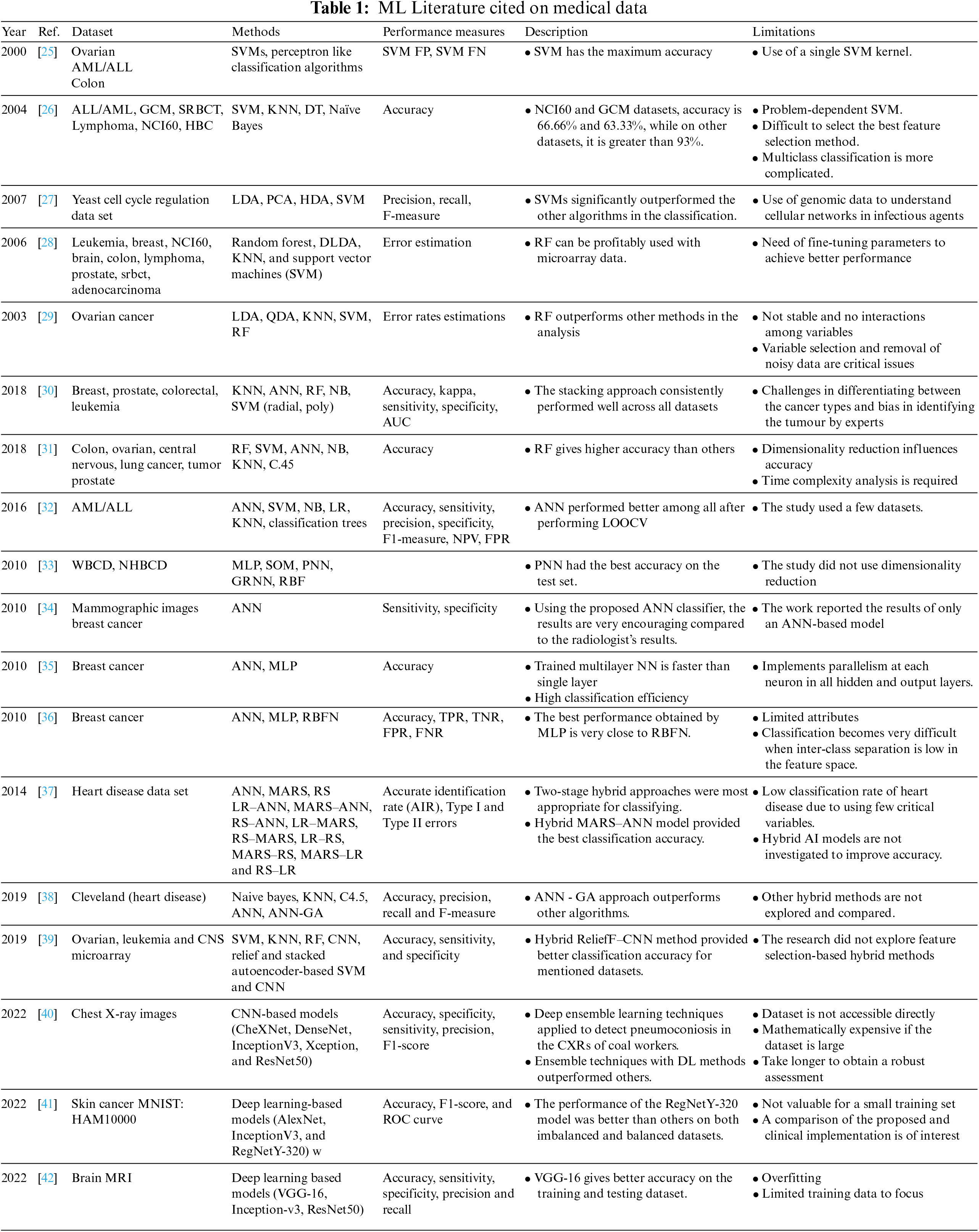
SVM [6] is increasingly becoming a standard learning algorithm in various research fields for scanning a hyperplane to categorize GE data within the margins of two classes. Similarly, Fisher’s LDA [5] model is also used to find linear sample arrangements to divide samples into two or more groups. Leo Breiman [7] has developed the RF classification algorithm based on ensemble learning, which has properties that make it desirable for the classification of GE microarray data by using random samples from the original data and constructing a chain of classification trees. The kNN method [8] is another method used for GE microarray data classification; it categorizes samples by evaluating the resemblance between sample pairs based on distance functions. Researchers use ANN for various optimization and mathematical problems such as classification, identification of objects and images, signal processing, prediction of seismic events, temperature and weather forecasting, bankruptcy, tsunami strength, earthquake, sea level, etc. [20–22]. Hybrid models for disease detection and classification were also proposed in the literature [23,24]; the table below shows various studies with their outcomes and limitations on datasets related to the medical field.

The literature shows that no work measures the initial weights for ANNs based on the outputs of the supervised classifiers. Therefore, to carry out the predictive analysis using the NN classifier, the present study uses the hybrid method by computing the initial weights using supervised-learning settings. For the description of the proposed technique, see the next section.

This paragraph describes the short form of the spelled-out abbreviations used in Table 1. Acute Myeloid Leukemia (AML), Acute Lymphocytic Leukemia (ALL), Global Cancer Map (GCM), Small Round Blue Cell Tumors (SRBCT), National Cancer Institute (NCI60), Home Based Primary Care (HBC), Decision Tree (DT), Principal Component Analysis (PCA), Heteroscedastic Discriminant Analysis (HDA), Diagonal Linear Discriminant Analysis (DLDA), Quadratic Discriminant Analysis (QDA), Naïve Bayes (NB), Area Under the Curve (AUC), Logistic Regression (LR), Negative Predictive Value (NPV), False Positive Rate (FPR), Leave One Out Cross Validation (LOOCV), Wisconsin Breast Cancer Diagnosis (WBCD), Namazi Hospital Breast Cancer Data (NHBCD), Multi-Layer Perceptron (MLP), Self-Organizing Map (SOM), Probabilistic Neural Network (PNN), General Regression Neural Network (GRNN), Radial Basis Function (RBF), Radial Basis Function Network (RBFN), True Positive Rate (TPR), True Negative Rate (TNR), False Negative Rate (FNR), Multivariate Adaptive Regression Splines (MARS), Rough Set (RS), Logistic Regression (LR-ANN), Artificial Neural Network-Genetic Algorithm (ANN-GA), Central Nervous System (CNS), Convolution Neural Network (CNN), Randomised Cross-Fold-Validation (RCFV), Chest X-Ray (CXR), Deep Learning (DL), Receiver Operating Characteristic (ROC), Magnetic Resonance Imaging (MRI), Visual Geometry Group (VGG-16), Residual Networks (Resnet).

3  Datasets and Methods

The upcoming section includes details about the methods used in the proposed study, along with datasets. This presented study uses two publicly available datasets, discussed in the datasets section, various traditional ML algorithms, and the proposed methodology. The last part of this section presents the evaluation metrics used to analyze the results.

3.1 Datasets

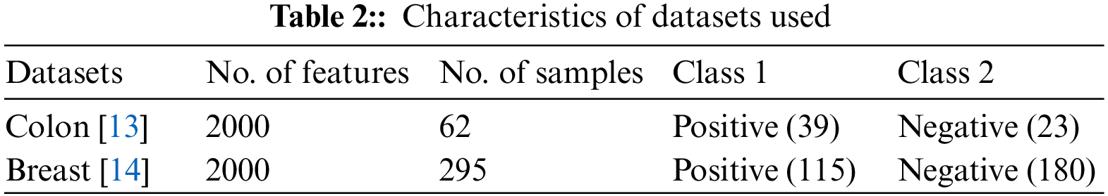
The current analysis uses two publicly available GE microarray datasets. The colon cancer dataset [13] includes a genetic profile of 39 patients with colon cancer and 23 healthy subjects. The factor grouping describes the patient status, and the numeric variables give the gene value. The breast cancer dataset [14] includes gene expression values for 295 breast cancer patients, of whom 115 were affected by the disease while 180 were healthy. Table 2 describes the characteristics of the datasets used in this research work.

3.2 Methodology

The proposed methodology, which works on supervised ML algorithms coupled with ANN, is presented in this section. ANN models accomplish the organization and functions of biological neural networks. ANN’s basic building blocks are artificial neurons. Inputs are weighted at the start of the artificial neuron by a product of each input and its weight. A function in the internal neuron sums up all weighted inputs and biases. The overview of previous weighted inputs and biases on output neurons are passed on to the activation function. The following equation indicates ANN products with k elements:

y(x)=∑i=1kwiyi(x)(1)

Here “yi” and “wi” are the output and weights at layer “i”, respectively.

This presented work uses the multilayer perceptron model of ANN. In MLP, like a multistage graph, neurons are organized into layers. Each node on each layer receives input from an associated node on the previous layer. It then calculates a function’s value and provides the computed value as an input to the linked node on the next layer, as depicted in Fig. 1. These layers are known as the input, hidden, and output layers. The intermediate layer does not connect with the initial input layer, and the final output layer is the hidden layer. In various fields, such as forecasting, economic modelling and medical applications, the neural network has widespread uses [43]. Several types of research relevant to cancer classification [32] and other bioinformatics fields [25] use ANN. Moreover, [44,45] discussed the additional utilities of ANN models.

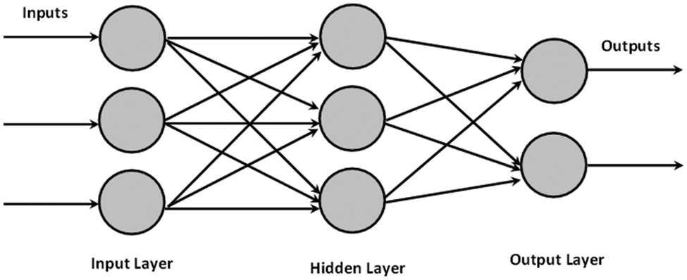
Figure 1: Artificial Neural Network with one hidden layer

Generally, in ANNs, there are different schemes for weights initialization, including zero, random, He, and Xavier initializations [10,11]. This work proposes to initialize the weights of inputs by computing them using a supervised framework. ML literature offers different supervised learning algorithms for predictive analysis [46,47]. However, studies show that the following learning algorithms suit GE microarray data-based predictive systems [48,49]. The learning algorithms used in this study to estimate the initial weights are as follows.

3.2.1 Support Vector Machines

The Support Vector Machine (SVM) was initially developed by Cortes et al. [6] to build predictive systems to solve problems using regression and classification methodologies. SVMs have been demonstrated to be successful in various pattern recognition tasks [50] and outperform other traditional classification algorithms. The variant of SVM for binary classification divides a group of training samples into two classes. One may define training samples as:

(x1,y1),(x2,y2),…,(xn,yn)(2)

Here, xi∈XD signifies vectors in a D dimensional feature space and yi∈{−1,+1} is a class label.

The SVM model is created by producing a new higher-dimensional feature space from the input samples indicated as φ:XD→HF, where D<F is the dimension of the input vectors. Then, the kernel function k(xi,xj), which is the product of input vectors xiand xj (k(xi,xj)=φ(xi).φ(xj)), generates an optimum separating hyperplane in the new feature space. In the literature, for SVMS several kernel functions have been proposed.

The technique of a linear kernel-based SVM maps the nonlinear input space into the new linearly separable space. All vectors on one side of the hyperplane are labelled “−1”, while all vectors on the other are labelled “+1”. Support vectors are the training examples in the converted space closest to the hyperplane. The margin of the hyperplane, and decision surface, is determined by the number of these support vectors, which is generally tiny compared to the size of the training set, as depicted in Fig. 2.

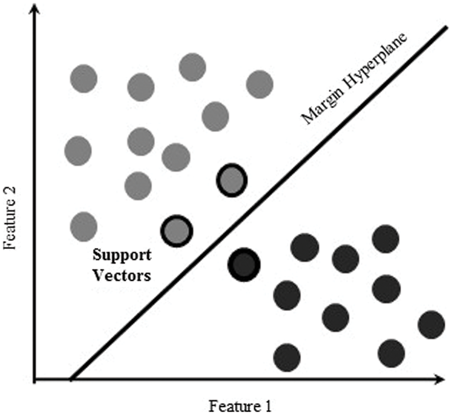
Figure 2: Support vector machine with linear separability

Other commonly used kernel functions are the Polynomial and Gaussian Radial Basis (RBF), which are kpoly(xi,xj)=(xi.xj+1)p, where p is the degree of the polynomial and kgaussian(xi,xj)=e‖(xi−xj‖22σ where σ is gaussian sigma, respectively.

According to the literature, there is no formal technique to determine the optimum kernel function for a given domain problem. However, linear, polynomial, and RBF kernels are the most widely used and compared among different kernel functions in various domain problems [51].

3.2.2 Linear Discriminant Analysis (LDA)

It is a classification system developed by R. A. Fisher in 1936 [5]. Numerous fields used this method, such as machine learning [49], identification of patterns [52] and statistically based research. This approach is mathematically stable and straightforward. It provides a model with good precision for finding linear arrangements of samples to distinguish them between two or more groups of events or objects. LDA is applicable for linear classification or dimension reduction.

LDA has also been used to find certain variables with a linear combination that helps distinguish two groups robustly, as illustrated in Fig. 3. Although LDA uses predictive classes, it is not considered a classifier. Still, the outcomes are known as part of the linear classification. Before using any alternative method, such as nonlinear techniques, it carries out dimensionality reduction. In GE microarray data processing, LDA is commonly used [27,49,53].

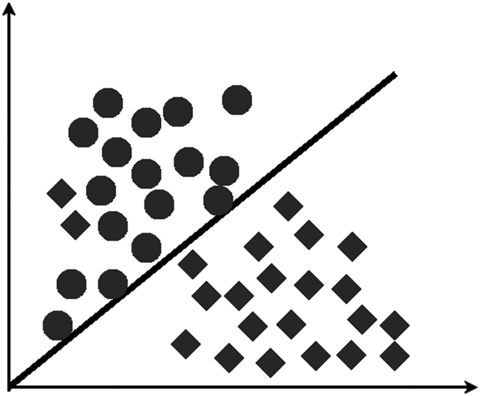
Figure 3: Linear discriminant analysis

3.2.3 Random Forest (RF)

A classifier consisting of a group of organized tree classifiers, such as

h(x,Θk),k=1,…(3)

is usually referred to as a random Forest where {Θk} is self-regulating identically distributed random vectors, and each tree casts a unit vote at the input x for the best standard class. In all these processes, the collective element is that a random vector Θk is produced for the kth tree sovereign over the previous random vectors. These steps make use of both equal circulation and training sets. Finally, based on Θk a tree is formed, generating a classifier h(x,Θk) where x represents an input vector. For instance, the M random vectors are generated in bagging as per the counts in N. Here, N represents the number of instances in the training set. A classifier is built and tested for each random vector M. Finally; the output is produced by aggregating the outputs of all the M. Fig. 4 portrays this process.

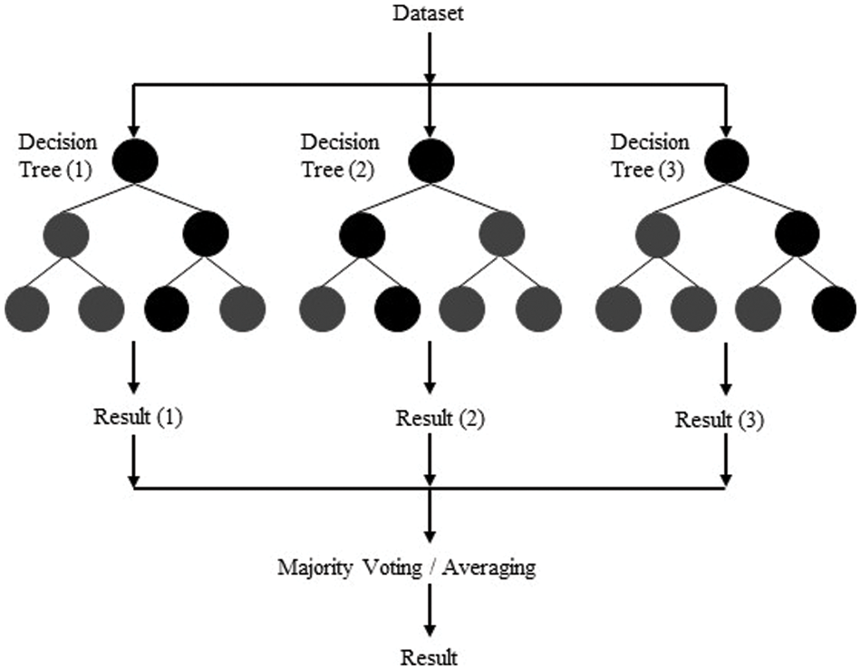
Figure 4: Random forest selection process

In the literature on machine learning, researchers use the random forest technique for gene selection and microarray data classification [49,54].

3.2.4 k-Nearest Neighbour

It is recognized that the k-nearest neighbour classifiers (kNN) are the most helpful example-based learners. kNN operates on the premise that examples are likely to fit into the same class of nearby space. Calculations that measure the distance between two points are Euclidian, Manhattan, Minkowski, etc. and their formulae are:

Euclidean=∑i=1n(xi−yi)2(4)

Manhattan=∑i=1n|xi−yi|(5)

Minkowski=(∑i=1n(|xi−yi|)q)1/q(6)

A kNN assigns the class that is most persistent among the neighbouring k samples. k is a control to fine-tune the algorithm for classification.

3.3 Working of Proposed Methodology

In ML, the process of cross-validation and classification is characterized by a series of steps, as illustrated in Fig. 5. Generally, a classification task considers a dataset having various samples and groups defined by the following relation.

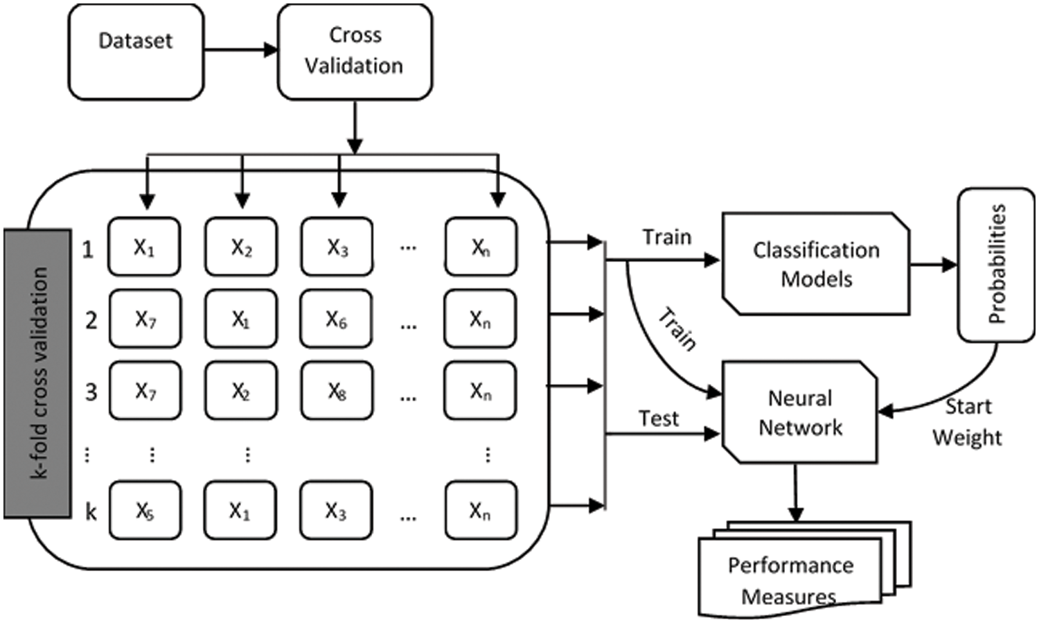
Figure 5: Proposed methodology

χ={xr,yr}r=1N(7)

Here, x represents the feature space, y represents the target, and r represents an example in the dataset χ. Targets may be categorical values (in the case of a classification problem) or continuous values (in the case of a regression problem).

Different models, each generating a classifier, are learned using learning algorithms (discussed in the next section). The purpose of the classifier is to measure the class association scores and assign to unseen samples a discrete class mark (from one of the target values), i.e.,

y=f(x)={123⋮(8)

Whereas in-case of binary classification, the target will be

y=f(x)={1ifx∈+iveclass0ifx∈−iveclass(9)

The train and test sets are obtained using the notion of CV after constructing folds. For this purpose, data is split into k-folds to provide a generalized predictive model (Fig. 5). In k-fold cross-validation, the data is first partitioned into k segments or folds of equal (or almost equal) size. Subsequently, k-training and test iterations are carried out so that a different fold of the data is kept out for testing within each iteration. In contrast, the remaining k−1 folds are used for learning.

The proposed method uses the training data set to build the predictive model and the test set to evaluate the performance of the constructed model. During the testing process, the method computes the scores of the class association of the test data set. Then, the neural network uses these scores as initial weights to build the predictive model. In the next step, the proposed method uses the performance measures (discussed later) to evaluate the built model., as shown in Fig. 5.

The error rate is the measure to gauge the efficiency of a classifier. If the classifier is not sufficiently accurate for the job, it is possible to consider other techniques. In this analysis, class association scores generated by predictive models built using traditional ML algorithms are used as initial weights to construct NN hybrid models, as demonstrated in Fig. 6.

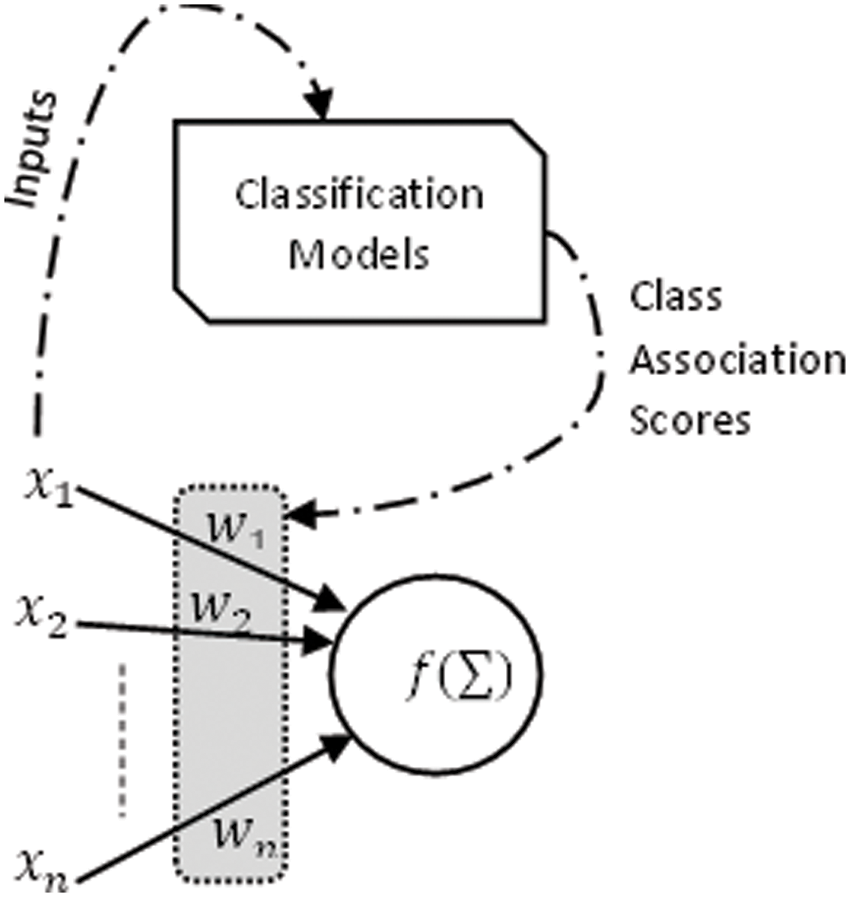
Figure 6: NN-based hybrid model

Factors w1,w2,…,wn are weights to determine the strength of input vectors X=[x1,x2,….xn]T. These weights are determined by conventional ML classifiers using the proposed process. Eq. (10) computes the product of each input and the associated neuron withXTw. The positive weights excite, while the negative weights inhibit node production.

X=XT.w=x1w1+x2w2+…+xnwn=∑i=1nxiwi(10)

The nodes’ interval threshold ɸ is the magnitude offset. It affects the activation of node output O as follows:

O=f(X)=f{∑i=1niiwi−Φk}(11)

ANN needs to be trained for the networks to generate the desired input-output mapping for the classification task. The neural network uses example data and link weights for training a model. These weights are measured and adapted using traditional ML algorithms (LDA, SVM, kNN, RF).

The proposed method utilizes the default values to initialize the rest of the parameters for neural network training, and all the outputs (possible system responses) have the same probability. The weights that define the relationships between nodes adjust the value during the network learning process, and it modifies the structure based on the input and hidden values. That means different neural network configurations are possible by changing the solution's steps and the mechanism of weights calculation.

For the training of ANN with m number of training data, the squared error can be given as

E=∑i=1m(ti−pi)2(12)

Here t is the performance goal, and p is the estimated output from training data. Different techniques have been used in the literature for optimal network efficiency when training ANNs, such as the Back Propagation Algorithm or Delta Rule. Studies reported in ML literature show that adjusting start weights to class association scores for classification has not yet been used in the ANN framework. The following algorithm summarizes the complete mechanism of the proposed study.

3.4 Algorithm

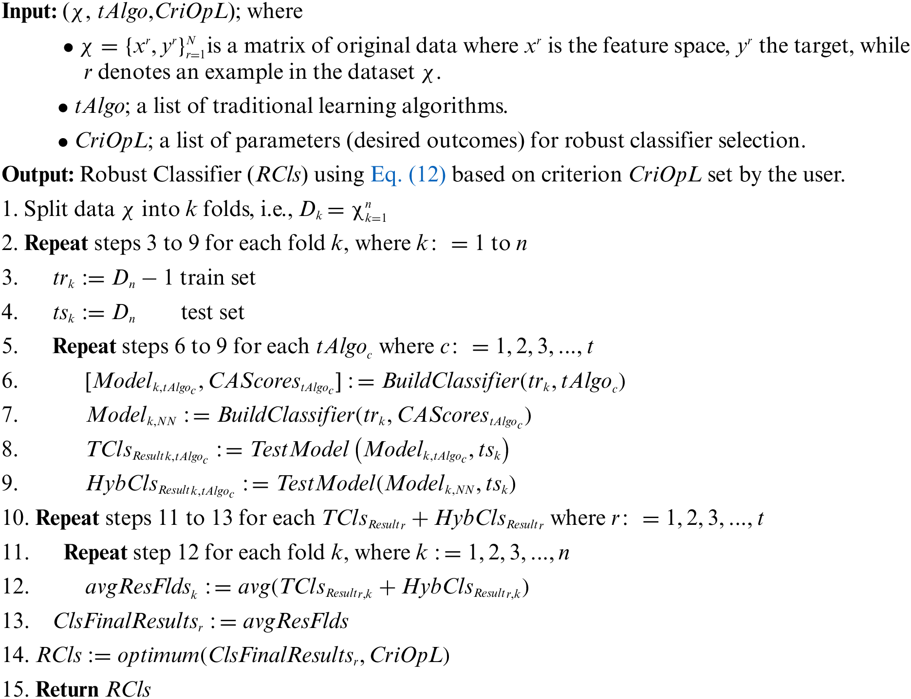
The algorithm starts by taking a matrix of original data (χ={xr,yr}r=1N) where xr is the feature space, yr is the target, and r represents an example in the dataset χ. The algorithm splits the original data χk=1n into k distinct folds (Dk). Please refer to line 1.

In lines 3–4, considering all k folds, alternatively, each fold is used as a test set (tsk) while the remaining folds are as a train set (trk). For each of the traditional learning algorithms TLAlgoc, a predictive model is learned (line 6), and the proposed model using ANN with class association scores (CAScores) as initial weights is also built (line 7). Lines 8–9 perform the testing of newly built models. For each combination of traditional and hybrid learning algorithms, from all k folds, the mean values of performance measures are calculated (refer to lines 10–12). Finally, from these average results, a robust classifier is obtained and returned using lines 14–15.

Generally, the efficiency of a classifier is calculated by the rate of misclassification or accuracy, although there are other ways to assess performance other than accuracy. Therefore, various parameters other than accuracy and error rate are also considered in this analysis to determine the classifier’s efficiency.

3.5 Evaluation Measures

The performance of a classification model is measured using a confusion matrix. This matrix represents the classification result in four categories: True Positive (TP), True Negative (TN), False Positive (FP), and False Negative (FN). Other evaluation metrics are formed based on these four categories.

3.5.1 Accuracy (ACC)

The quintessential classification metric is accuracy. Accuracy is the proportion of correct predictions among the total cases evaluated. It is suitable for binary and multiclass classification problems and is quite simple to comprehend. It can be computed from the following equation using the well-established notion of a confusion matrix.

Accuracy=(TP+TN)/(TP+FP+FN+TN)(13)

3.5.2 Sensitivity (SN)

Sensitivity (recall) refers to how many of the actual positive cases the constructed model was able to predict accurately. It is a remarkable statistic that FN is more concerned than FP. It is critical in medical situations when it does not matter whether it raises a false alert; the TP cases should not go unnoticed. It is the ratio of the total number of TP to the total number of actual positives.

Sensitivity(Recall)=TP/(TP+FN)(14)

3.5.3 Specificity (SP)

Specificity is the proportion of TN to all adverse outcomes. This measure is helpful if the accuracy of the negative rate is of interest and a positive output comes at a high cost. The following formula computes specificity:

Specificity=TN/(TN+FP)(15)

3.5.4 Precision (PREC)

Precision reveals how many of the accurately predicted instances turned out to be positive in the end. The precision measure becomes a handy tool when FP is more of a problem than FN. The number of TP divided by the number of predicted positives is the precision of a label.

Precision=TP/(TP+FP)(16)

3.5.5 Lift

The ML algorithms employed to solve classification problems often yield a probability. The algorithms use this probability to make the final prediction. The lift curve uses this returning probability to evaluate how effectively the model detects positive and negative instances in data sets. Lift compares prediction performance to randomly generated predictions in the classification domain using the following relation:

Lift=(TP/(TP+FP))(TP+FN)/(TP+FP+FN+TN)(17)

3.5.6 F-Measure

It is the harmonic mean of precision and recall. It is critical to use if a data set’s class distribution is unequal and the cost of FP and FN differs. The F-score represents the balance between recall and precision. If there is a balance between Precision and Recall, F-measure is higher, and if one of these metrics increases at the expense of the other, it does not become too high.

FMeasure=2∗(Recall∗Precision)/(Recall+Precision)(18)

3.5.7 Matthews Correlation Coefficient (MCC)

The MCC assesses the relationship between actual and predicted classes. Its range is [−1,+1], with −1 denoting perfect misclassification and +1 denoting perfect classification, whereas MCC = 0 represents random guessing. MCC would return a high score only if the prediction performed well in all of the confusion matrix groups (TP, FP, TN, FN) proportionally to the size of positive and negative elements in the data set. Therefore, it is encouraged to consider this evaluation metric in ML and data science projects.

MCC=(TP∗TN)−(FP∗FN)(TP+FP)(TP+FN)(TN+FP)(TN+FN)(19)

3.5.8 Area Under the Curve (AUC)

The AUC measures a classifier's ability to discriminate between classes. The AUC indicates how well the model performs at different threshold points between positive and negative class samples. The higher the AUC, the better the performance of the model. When AUC is equal to 1, the classifier can correctly discriminate between all positive and negative class points. When the AUC is zero, the classifier predicts all negatives as positives and vice versa. The classifier cannot discriminate between the positive and negative classes when AUC equals 0.5.

3.5.9 Kappa

Like classification accuracy, Cohen's Kappa (or simply Kappa) is standardized at the baseline of the random chance of a dataset. It is a better metric to utilize when there is an unequal distribution of classes. In classification, Kappa is a measure of agreement between observed and predicted or inferred class predictions for instances in a test data set. Its definition is as follows:

Kappa=(totalaccuracy–randomaccuracy)/(1−randomaccuracy)(20)

where random accuracy is defined as the sum of the products of reference likelihood and resultant likelihood for each class label.

Other performance metrics calculated from the confusion matrix include Negative Predictive Value (NPV), False Positive Rate (FPR), False Discovery Rate (FDR), and False Negative Rate (FNR).

4  Results and Discussion

This study assesses the exhibition of various ML classifiers to improve the classification ability of the traditional NN model through hybridization mechanisms. Experiments performed on cancer datasets are used to compile the results (based on several evaluation measures) of the proposed hybrid models, the traditional ML and the traditional ANN-based classifiers. For each model, this study evaluated the ACC, SN, SP, Kappa, PREC, MCC, AUC, Lift, F-Measure, and other metrics using Eqs. (13)–(20), respectively. Each experiment uses parameter optimization and 10-fold cross-validation to avoid overfitting. Tables 3–6 show the performances of traditional and hybrid models using obtained evaluation metrics.

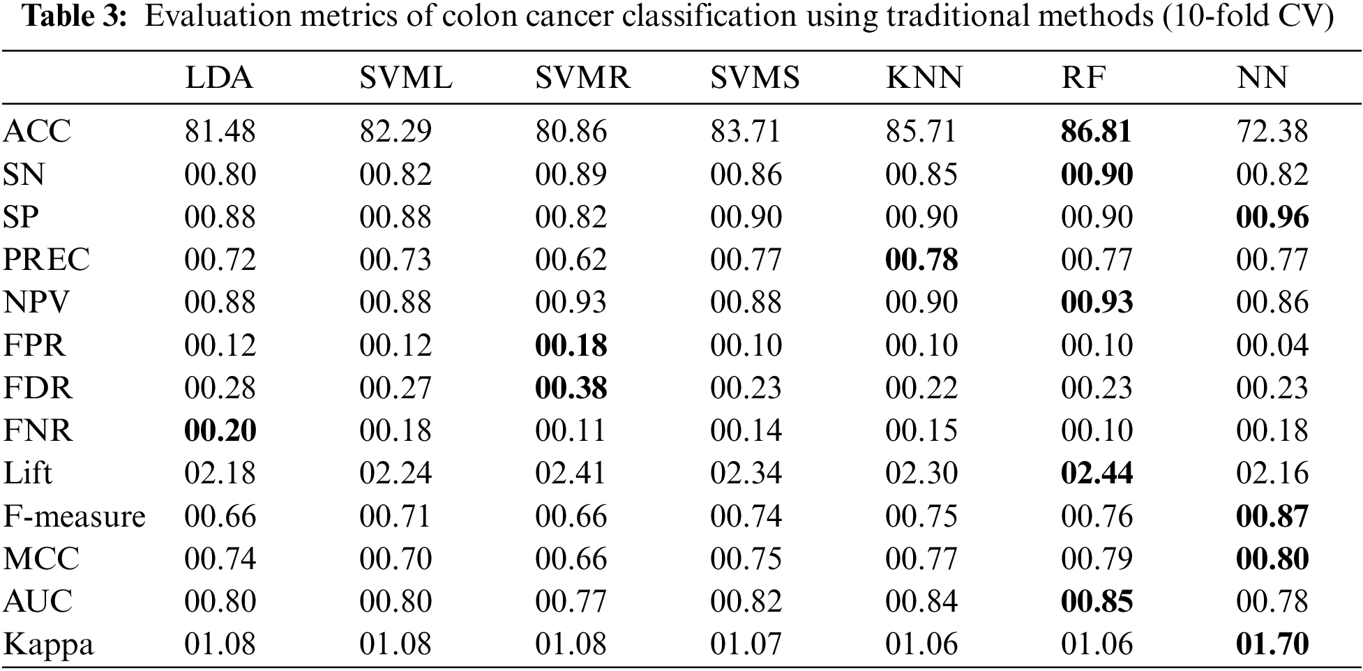
4.1 Colon Cancer Result Evaluation

The results in Table 3 show that different traditional ML classifiers performed well on the Colon cancer dataset. ANN classifier achieves the maximum SP (00.96), F-measure (00.87), MCC (00.80) and Kappa (01.70), followed by the RF classifier. Similarly, RF obtained the highest ACC (86.81%), highest SN (00.89), lowest NPV (0.92), and highest lift (02.44); additionally, the AUC curve for the RF classifier is around 0.84.

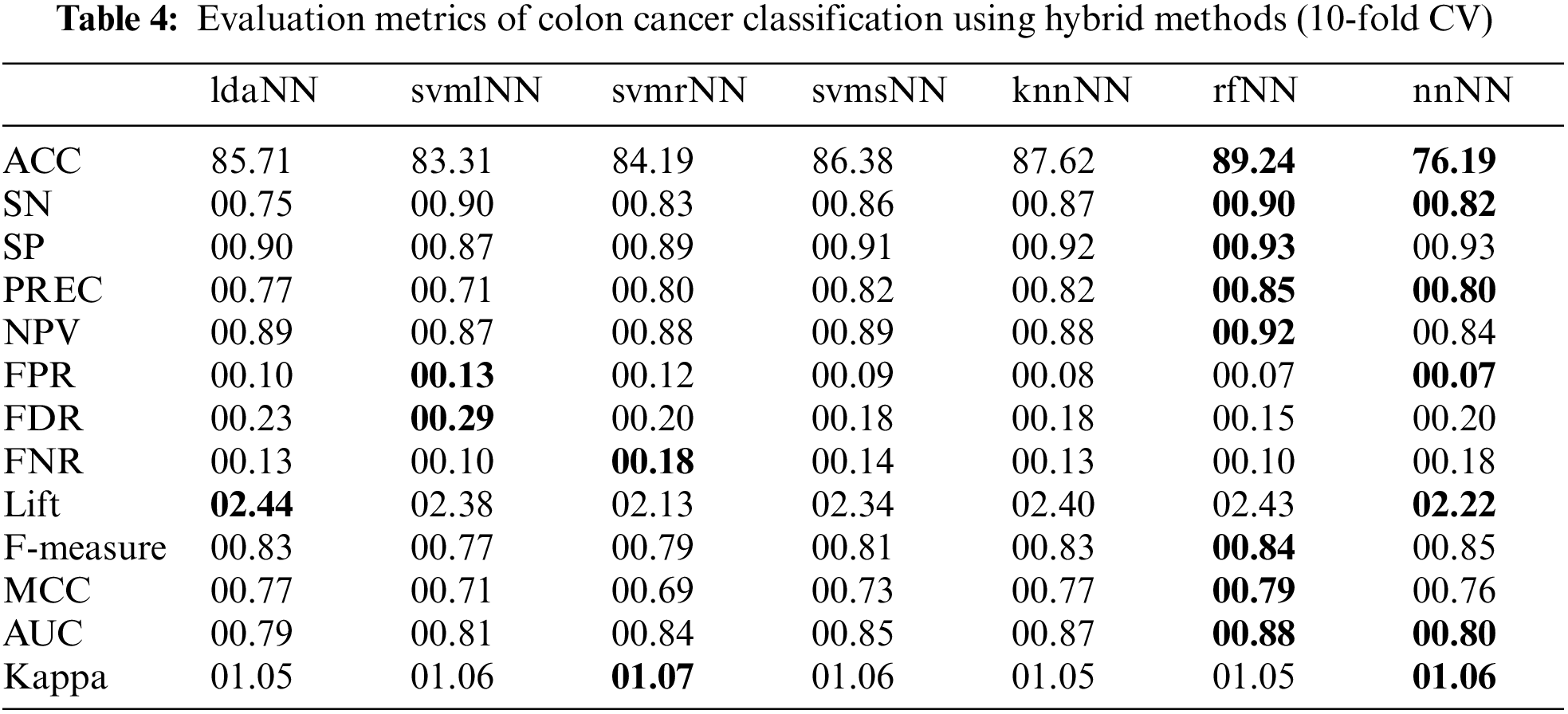
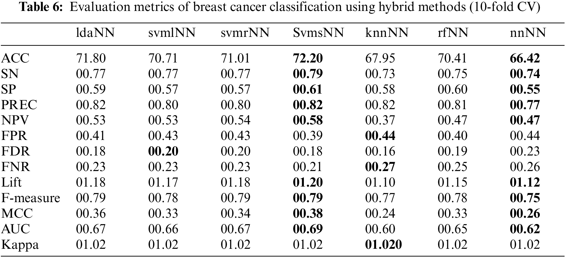
Tables 4 and 6 show the results of hybrid models. In these tables, the names of hybrid models consist of lowercase letters followed by capital letters. The lowercase letters refer to the traditional ML algorithms used to compute the class association scores. In contrast, the capital letters (NN) refer to the neural network model. Here, the scores from traditional ML algorithms are used in NN to build the hybrid models. The results show that rfNN achieved a better accuracy of (89.24%) compared to other hybrid and traditional models, as shown in Fig. 7. Similarly, the SN and SP obtained by rfNN were 00.89 and 00.93, where svmlNN provided the maximum of (00.89) SN and knnNN reached 00.92 SP. Moreover, the maximum separation obtained by rfNN is 00.88, whereas knnNN has an AUC value equal to 00.87. Similarly, for imbalanced data, the MCC is a better evaluation metric; rfNN obtained (00.79) MCC value compared to other hybrid classifiers. rfNN provides a better F-measure and NPV value of 00.84 and 00.91, respectively. In the case of performance metrics other than the ones mentioned above, svmlNN obtains the highest values of FPR (00.13) and FDR (00.28) , whereas svmrNN provides FNR (00.17) and Kappa (01.06). For a detailed view of metric values, refer to Table 4.

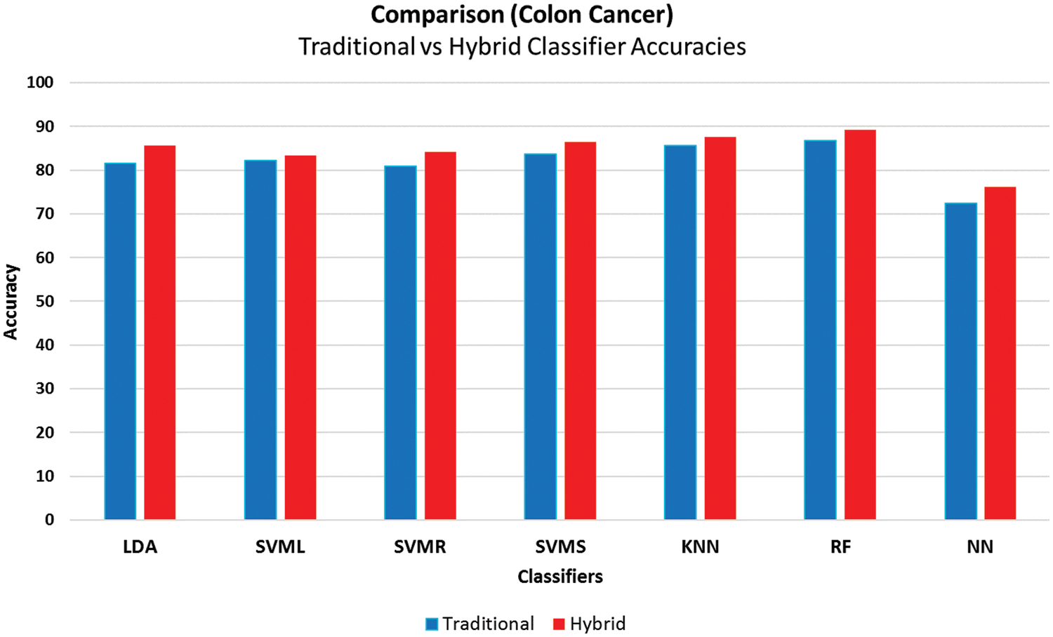
Figure 7: Accuracies comparison of traditional and the proposed framework using the colon cancer dataset

The comparison of the misclassification rate indicates that all the hybrid models built using the proposed framework outperformed the traditional approaches (Fig. 7). The proposed hybrid framework also has reasonably good F-measures above 00.80 other than svmlNN, which indicates quite good performance.

Results using the proposed framework on the Colon cancer gene expression dataset indicate that the rfNN model from hybrid methods performed best with the proposed approach with the minimum errors reported with tenfold cross-validation. Moreover, in all cases, hybrid models have better results than traditional methods.

4.2 Breast Cancer Result Evaluation

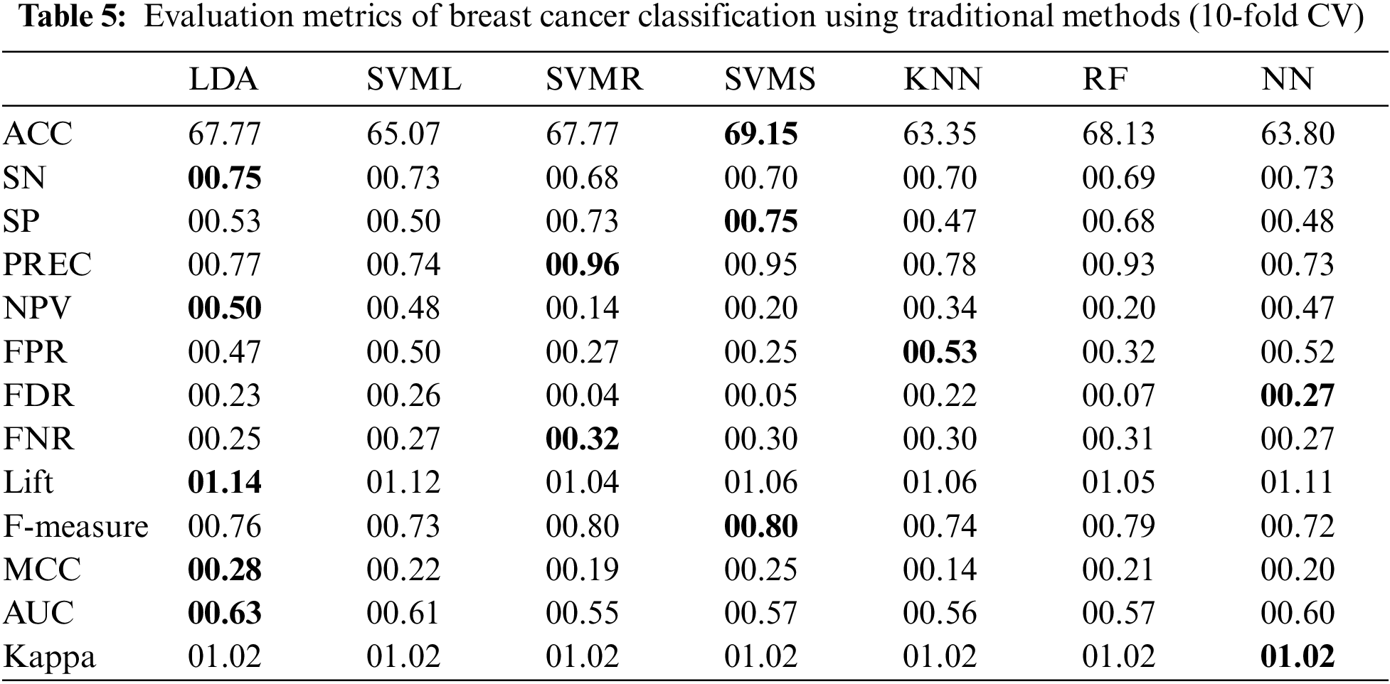
This section presents the results obtained from the experiments of the proposed methodology using the breast cancer dataset. The results are shown in Table 5 for traditional and Table 6 for hybrid methods.

The results in Table 5 show that using traditional ML classifiers on the breast cancer dataset, SVMS provides a maximum accuracy of 69.15% and the highest F-Measure and SP of 00.80 and 00.75, respectively. LDA provides a better AUC of 00.63 with an MCC equal to 00.28, followed by SVMS, which has an MCC value of 00.25. Moreover, LDA has greater values for Lift (01.14), NPV (00.50) and SN (0.75). In the case of Precision and FNR, SVMR performs better, and NN has values of 00.27 and 01.02 for FDR and Kappa, respectively.

Table 6 contains the outcomes of hybrid models. The results show that svmsNN outperforms all the other hybrid models and gives better values for most performance metrics. It predicts a better accuracy of 72.20% along with max values of SN (00.79), SP (00.61), PREC (00.82), NPV (00.58), Lift (01.20), F-measure (0.79), MCC (00.38) and AUC (00.69). The knnNN has the highest value for FPR (00.44), Kappa (01.02) and FNR (00.27).

Fig. 8 compares the accuracies of traditional and hybrid models, showing that the hybrid models built using the proposed framework have better accuracy in all the cases. The hybrid ML techniques also have a reasonably good MCC above 00.30 other than knnNN, which has an excellent performance in imbalanced classification problems.

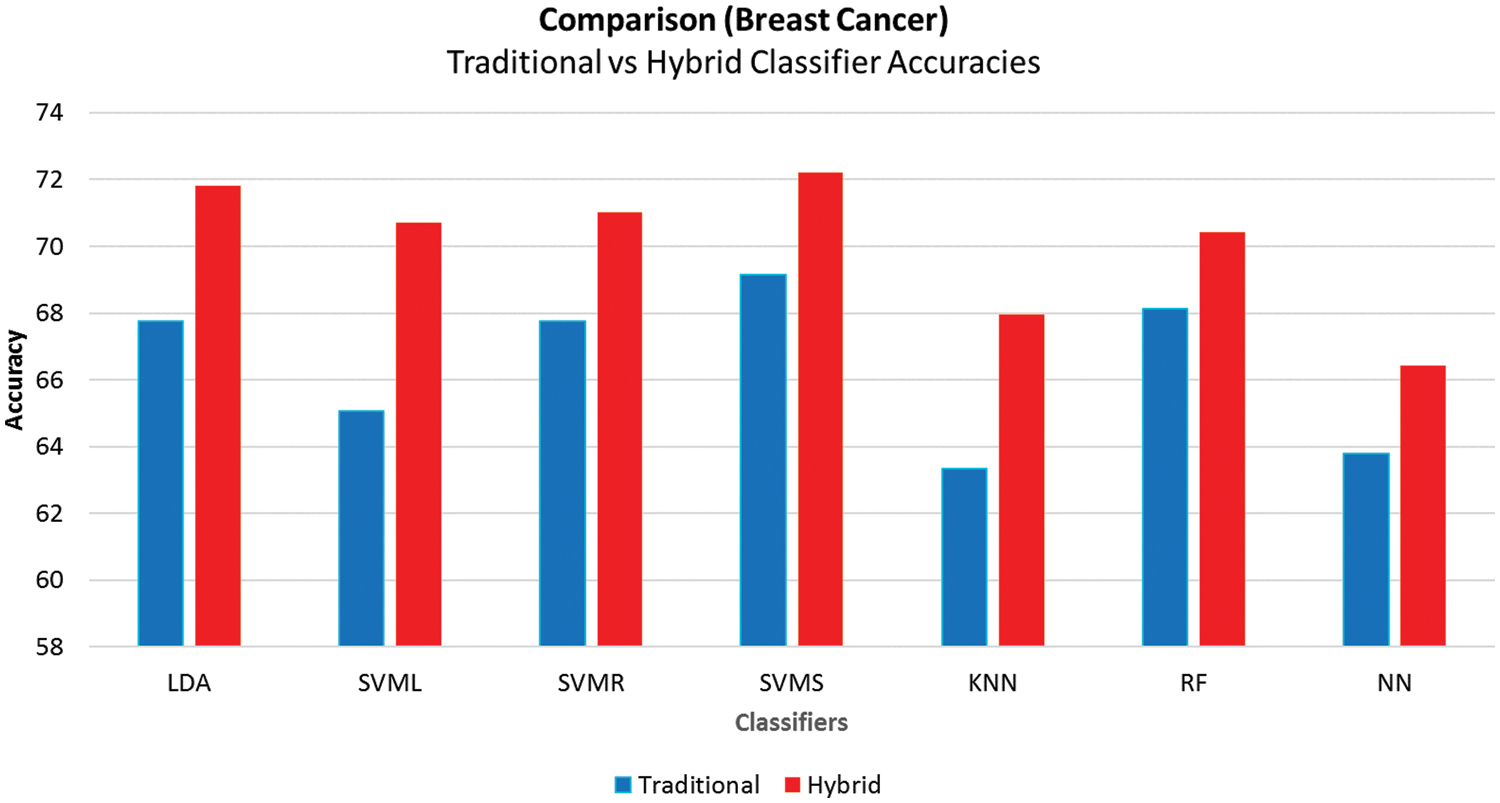
Figure 8: Average accuracies comparison of breast cancer

Overall results indicate that hybrid models have better results than other methods. The svmsNN model from the hybrid ML models performed best with the proposed approach with minimum errors, as reported with tenfold cross-validation.

5  Conclusion

Neural network-based prediction models are considered the most appropriate models in the ML domain. Initial weights are one of the most critical factors affecting NN-based models’ performance. The most widely used method to initialize the initial weights is random initialization. This study proposes to have initial scores computed by traditional ML algorithms rather than initializing them with random numbers. The hypothesis was that the more realistic initial weights this study has, the more accurate the NN-based models would be. This study used two publicly available GE microarray datasets to test the proposed framework. The reported results based on confusion matrix-based measures show the usefulness of the proposed framework.

Overall results indicate that the rfNN and svmsNN models from the hybrid framework performed better than traditional approaches on the colon and breast cancer datasets with minimum errors, as reported with tenfold cross-validation. Moreover, hybrid models have better results than other ANN-based methods used in this study.

6  Future Directions

This study exemplifies the solicitation of supervised machine learning methodologies for classifying cancerous datasets by utilizing microarray gene expression profiles of samples. The comparison and analysis of obtained results based on predictive models show the usefulness of the proposed method. This classification framework requires no selection of gene features and gives acceptable accuracy.

This work presents a step forward in the prediction of various types of cancer. Numerous investigators have worked on this as a binary classification task and achieved different precisions. Although this study shows that the proposed framework performs better than traditional approaches, certain aspects are still unexplored. For example, the applications of the proposed framework in areas other than GE microarray analysis require investigation. Moreover, the impacts of using the proposed framework with different activation functions may be of interest.

Acknowledgement: The authors thank Aliya Shaheen, Assistant Professor (Mathematics), for her support and guidance during this study.

Funding Statement: The authors received no specific funding for this study.

Conflicts of Interest: The authors declare they have no conflicts of interest to report regarding the present study.

References

1. B. Van Calster, D. J. McLernon, M. Van Smeden, L. Wynants and E. W. Steyerberg, “Calibration: The Achilles heel of predictive analytics,” BMC Medicine, vol. 17, no. 1, pp. 1–7, 2019. [Google Scholar]

2. J. Hathaliya, P. Sharma, S. Tanwar and R. Gupta, “Blockchain-based remote patient monitoring in healthcare 4.0,” in IEEE 9th Int.Conf. on Advanced Computing (IACC), Tiruchirappalli, India, pp. 87–91, 2019. [Google Scholar]

3. M. J. Druzdzel and R. R. Flynn, “Decision support systems. Encyclopedia of library and information science. A. Kent,” Marcel Dekker, Inc. Last Login, vol. 10, no. 3, pp. 2010, 1999. [Google Scholar]

4. O. Adir, M. Poley, G. Chen, S. Froim, N. Krinsky et al., “Integrating artificial intelligence and nanotechnology for precision cancer medicine,” Advanced Materials, vol. 32, no. 13, pp. 1901989, 2020. [Google Scholar]

5. R. A. Fisher, “The use of multiple measurements in taxonomic problems,” Annals of Eugenics, vol. 7, no. 2, pp. 179–188, 1936. [Google Scholar]

6. C. Cortes and V. Vapnik, “Support-vector networks,” in Machine learning, vol. 20, Boston, MA: Kluwer Academic Publisher, pp. 237–297, 1995. [Google Scholar]

7. L. Breiman, “Random forests,” Machine Learning, vol. 45, no. 1, pp. 5–32, 2001. [Google Scholar]

8. N. S. Altman, “An introduction to kernel and nearest-neighbor nonparametric regression,” The American Statistician, vol. 46, no. 3, pp. 175–185, 1992. [Google Scholar]

9. W. S. McCulloch and W. Pitts, “A logical calculus of the ideas immanent in nervous activity,” The Bulletin of Mathematical Biophysics, vol. 5, no. 4, pp. 115–133, 1943. [Google Scholar]

10. S. Masood and P. Chandra, “Training neural network with zero weight initialization,” in Proc. of the CUBE Int. Information Technology Conf., Pune, India, pp. 235–239, 2012. [Google Scholar]

11. S. K. Kumar, “On weight initialization in deep neural networks,” arXiv preprint arXiv:1704.08863, pp. n.p, 2017. [Google Scholar]

12. M. Daoud and M. Mayo, “A survey of neural network-based cancer prediction models from microarray data,” Artificial Intelligence in Medicine, vol. 97, no. 12, pp. 204–214, 2019. [Google Scholar] [PubMed]

13. U. Alon, N. Barkai, D. A. Notterman, K. Gish, S. Ybarra et al., “Broad patterns of gene expression revealed by clustering analysis of tumor and normal colon tissues probed by oligonucleotide arrays,” Proc. of the National Academy of Sciences, vol. 96, no. 12, pp. 6745–6750, 1999. [Google Scholar]

14. M. J. Van De Vijver, Y. D. He, L. J. Van’t Veer, H. Dai, A. A. Hart et al., “A gene-expression signature as a predictor of survival in breast cancer,” New England Journal of Medicine, vol. 347, no. 25, pp. 1999–2009, 2002. [Google Scholar] [PubMed]

15. H. Fathi, H. AlSalman, A. Gumaei, I. I. Manhrawy, A. G. Hussien et al., “An efficient cancer classification model using microarray and high-dimensional data,” Computational Intelligence and Neuroscience, vol. 2021, no. 12, pp. n.p, 2021. [Google Scholar]

16. R. Bharti, A. Khamparia, M. Shabaz, G. Dhiman, S. Pande et al., “Prediction of heart disease using a combination of machine learning and deep learning,” Computational Intelligence and Neuroscience, vol. 2021, no. 11, pp. n.p, 2021. [Google Scholar]

17. M. N. Wernick, Y. Yang, J. G. Brankov, G. Yourganov and S. C. Strother, “Machine learning in medical imaging,” IEEE Signal Processing Magazine, vol. 27, no. 4, pp. 25–38, 2010. [Google Scholar] [PubMed]

18. E. Alpaydin, Introduction to Machine Learning. Cambridge, Massachusetts: The MIT Press, 2020. [Google Scholar]

19. J. G. Greener, S. M. Kandathil, L. Moffat and D. T. Jones, “A guide to machine learning for biologists,” Nature Reviews Molecular Cell Biology, vol. 23, no. 1, pp. 40–55, 2022. [Google Scholar] [PubMed]

20. C. Guojin, Z. Miaofen, Y. Honghao and L. Yan, “Application of neural networks in image definition recognition,” in 2007 IEEE Int. Conf. on Signal Processing and Communications, Dubai, UAE, pp. 1207–1210, 2007. [Google Scholar]

21. M. Romano, S. -Y. Liong, M. T. Vu, P. Zemskyy, C. D. Doan et al., “Artificial neural network for tsunami forecasting,” Journal of Asian Earth Sciences, vol. 36, no. 1, pp. 29–37, 2009. [Google Scholar]

22. M. Hayati and Z. Mohebi, “Application of artificial neural networks for temperature forecasting,” International Journal of Electrical and Computer Engineering, vol. 1, no. 4, pp. 662–666, 2007. [Google Scholar]

23. M. Khushi, K. Shaukat, T. M. Alam, I. A. Hameed, S. Uddin et al., “A comparative performance analysis of data resampling methods on imbalance medical data,” IEEE Access, vol. 9, pp. 109960–109975, 2021. [Google Scholar]

24. T. M. Alam, K. Shaukat, H. Mahboob, M. U. Sarwar, F. Iqbal et al., “A machine learning approach for identification of malignant mesothelioma etiological factors in an imbalanced dataset,” The Computer Journal, vol. 65, no. 7, pp. 1740–1751, 2002. [Google Scholar]

25. T. S. Furey, N. Cristianini, N. Duffy, D. W. Bednarski, M. Schummer et al., “Support vector machine classification and validation of cancer tissue samples using microarray expression data,” Bioinformatics, vol. 16, no. 10, pp. 906–914, 2000. [Google Scholar] [PubMed]

26. T. Li, C. Zhang and M. Ogihara, “A comparative study of feature selection and multiclass classification methods for tissue classification based on gene expression,” Bioinformatics, vol. 20, no. 15, pp. 2429–2437, 2004. [Google Scholar] [PubMed]

27. Y. Lu, Q. Tian, M. Sanchez, J. Neary, F. Liu et al., “Learning microarray gene expression data by hybrid discriminant analysis,” IEEE MultiMedia, vol. 14, no. 4, pp. 22–31, 2007. [Google Scholar]

28. R. Díaz-Uriarte and S. A. De Andres, “Gene selection and classification of microarray data using random forest,” BMC Bioinformatics, vol. 7, no. 1, pp. 1–13, 2006. [Google Scholar]

29. B. Wu, T. Abbott, D. Fishman, W. McMurray, G. Mor et al., “Comparison of statistical methods for classification of ovarian cancer using mass spectrometry data,” Bioinformatics, vol. 19, no. 13, pp. 1636–1643, 2003. [Google Scholar] [PubMed]

30. M. Mohammed, H. Mwambi, B. Omolo and M. K. Elbashir, “Using stacking ensemble for microarray-based cancer classification,” in 2018 Int. Conf. on Computer, Control, Electrical, and Electronics Engineering (ICCCEEE), Khartoum, Sudan, pp. 1–8, 2018. [Google Scholar]

31. H. Aydadenta and Adiwijaya, “On the classification techniques in data mining for microarray data classification,” in Journal of Physics: Conf. Series, Telkom University, Indonesia, vol. 971, pp. 12004, 2018. [Google Scholar]

32. A. K. Dwivedi, “Artificial neural network model for effective cancer classification using microarray gene expression data,” Neural Computing and Applications, vol. 29, no. 12, pp. 1545–1554, 2018. [Google Scholar]

33. A. S. Sarvestani, A. Safavi, N. Parandeh and M. Salehi, “Predicting breast cancer survivability using data mining techniques,” in 2010 2nd Int. Conf. on Software Technology and Engineering, San Juan, PR, USA, vol. 2, pp. V2–227, 2010. [Google Scholar]

34. M. J. Islam, M. Ahmadi and M. A. Sid-Ahmed, “An efficient automatic mass classification method in digitized mammograms using artificial neural network5129, arXiv, preprint arXiv:1007.5129, pp. n.p, 2010. [Google Scholar]

35. K. U. Rani, “Parallel approach for diagnosis of breast cancer using neural network technique,” International Journal of Computer Applications, vol. 10, no. 3, pp. 1–5, 2010. [Google Scholar]

36. R. Janghel, A. Shukla, R. Tiwari and R. Kala, “Breast cancer diagnosis using artificial neural network models,” in The 3rd Int. Conf. on Information Sciences and Interaction Sciences, Chengdu, China, pp. 89–94, 2010. [Google Scholar]

37. Y. E. Shao, C. -D. Hou and C. -C. Chiu, “Hybrid intelligent modeling schemes for heart disease classification,” Applied Soft Computing, vol. 14, no. Part A, pp. 47–52, 2014. [Google Scholar]

38. M. Akgül, Ö.E. Sönmez and T. Özcan, “Diagnosis of heart disease using an intelligent method: A hybrid ANN-GA approach,” in Int. Conf. on Intelligent and Fuzzy Systems, Istanbul, Turkey, Cham, Springer, pp. 1250–1257, 2019. [Google Scholar]

39. S. Kilicarslan, K. Adem and M. Celik, “Diagnosis and classification of cancer using hybrid model based on ReliefF and convolutional neural network,” Medical Hypotheses, vol. 137, no. 5439, pp. 109577, 2020. [Google Scholar] [PubMed]

40. L. Devnath, S. Luo, P. Summons, D. Wang, K. Shaukat et al., “Deep ensemble learning for the automatic detection of pneumoconiosis in coal worker’s chest x-ray radiography,” Journal of Clinical Medicine, vol. 11, no. 18, pp. 5342, 2022. [Google Scholar] [PubMed]

41. T. M. Alam, K. Shaukat, W. A. Khan, I. A. Hameed, L. A. Almuqren et al., “An efficient deep learning-based skin cancer classifier for an imbalanced dataset,” Diagnostics, vol. 12, no. 9, pp. 2115, 2022. [Google Scholar] [PubMed]

42. C. Srinivas, N.P. KS., M. Zakariah, Y. A. Alothaibi, K. Shaukat et al., “Deep transfer learning approaches in performance analysis of brain tumor classification using MRI images,” Journal of Healthcare Engineering, vol. 2022, no. 2, pp. 1–17, 2022. [Google Scholar]

43. A. Bahrammirzaee, “A comparative survey of artificial intelligence applications in finance: Artificial neural networks, expert system and hybrid intelligent systems,” Neural Computing and Applications, vol. 19, no. 8, pp. 1165–1195, 2010. [Google Scholar]

44. A. K. Dwivedi, “Performance evaluation of different machine learning techniques for prediction of heart disease,” Neural Computing and Applications, vol. 29, no. 10, pp. 685–693, 2018. [Google Scholar]

45. R. Yasdi, “A literature survey on applications of neural networks for human-computer interaction,” Neural Computing and Applications, vol. 9, no. 4, pp. 245–258, 2000. [Google Scholar]

46. F. Rustam, A. A. Reshi, A. Mehmood, S. Mehmood, B. -W. Mehmood et al., “COVID-19 future forecasting using supervised machine learning models,” IEEE Access, vol. 8, pp. 101489–101499, 2020. [Google Scholar]

47. S. Uddin, A. Khan, M. E. Hossain and M. A. Moni, “Comparing different supervised machine learning algorithms for disease prediction,” BMC Medical Informatics and Decision Making, vol. 19, no. 1, pp. 1–16, 2019. [Google Scholar]

48. L. Kumar and R. Greiner, “Gene expression based survival prediction for cancer patients—A topic modeling approach,” PloS One, vol. 14, no. 11, pp. e0224446, 2019. [Google Scholar] [PubMed]

49. M. H. Waseem, M. S. A. Nadeem, A. Abbas, A. Shaheen, W. Aziz et al., “On the feature selection methods and reject option classifiers for robust cancer prediction,” IEEE Access, vol. 7, pp. 141072–141082, 2019. [Google Scholar]

50. H. Byun and S. -W. Lee, “A survey on pattern recognition applications of support vector machines,” International Journal of Pattern Recognition and Artificial Intelligence, vol. 17, no. 3, pp. 459–486, 2003. [Google Scholar]

51. S. R. Das, K. Das, D. Mishra, K. Shaw and S. Mishra, “An empirical comparison study on kernel based support vector machine for classification of gene expression data set,” Procedia Engineering, vol. 38, pp. 1340–1345, 2012. [Google Scholar]

52. Z. B. Lahaw, D. Essaidani and H. Seddik, “Robust face recognition approaches using PCA, ICA, LDA based on DWT, and SVM algorithms,” in 2018 41st Int. Conf. on Telecommunications and Signal Processing (TSP), Athens, Greece, pp. 1–5, 2018. [Google Scholar]

53. M. S. A. Nadeem, J. -D. Zucker and B. Hanczar, “Accuracy-rejection curves (ARCs) for comparing classification methods with a reject option,” Journal of Machine Learning Research (JMLRW&CP, vol. 8, pp. 65–81, 2010. [Google Scholar]

54. K. Moorthy and M. S. Mohamad, “Random forest for gene selection and microarray data classification,” in Knowledge Technology Week, Vol. 295, Berlin, Heidelberg: Springer, pp. 174–183, 2011. [Google Scholar]