Effectiveness of Deep Learning Models for Brain Tumor Classification and Segmentation

1  Introduction

Brain tumors are a significant cause of death for both children and adults. When cells grow abnormally, abnormal tissue expansions occur, and that fibrous web of uncontrolled tissue that expands uncontrollably is known as a tumor or neoplasm [1]. The brain controls the functionality of the other body organs and decision-making and the completion of intentional and unintentional functions performed by the human body [2]. A tumor can raise the pressure inside the skull, disrupt the brain’s standard functionality, and be life-threatening, whether cancerous or non-cancerous [3].

Every year almost 11,000 people across the globe are diagnosed with deadly diseases and brain tumors. Nearly 500 of them are youngsters on average; it takes the lives of almost 5000 people [4]. Benign and Malignant are two classifications of brain tumors. A benign brain tumor is uniform in structure and does not contain active cells; hence it is not cancerous. On the other hand, a malignant tumor is cancerous and heterogeneous (non-uniform) in its structure. Benign tumors, low-grade tumors, are further categorized as Gliomas and Meningiomas. Glioblastoma and Astrocytoma are a sub-category of high-grade tumors. According to World Health Organization (WHO) and American Brain Tumor Association, to distinguish benign and malignant tumor types, a scale from grade I to grade IV is used [5].

Magnetic Resonance Imaging (MRIs), Computed Tomography (CT), X-rays, and Ultrasound are different medical imaging techniques and methods used for patient diagnosis and treatment with significant impact [6]. In neurology, Magnetic Resonance Imaging (MRI) is used to get the tiniest detail within the human body. MRI is commonly used to diagnose brain lesions and other abnormalities. MRI can visualize anatomy in all three planes: coronal, axial, and sagittal, and can offer precise detail of spinal cord, brain, and vascular anatomy. Segmentation is performed to differentiate healthy tissues from an area with a tumor, improving the chances of effective and successful tumor treatment. The image is separated into regions based on identical properties like boundaries, grey level, contrast, and texture [7]. Manually examining MRI images of the patient is a hectic job for a neurologist. The results obtained from a manual examination may have several flaws influencing the need for an automatic detection system. For segmentation purposes, partially automatic and fully automatic techniques and methods are used [8]. For cancer diagnosis and treatment, segmenting the tumor is crucial. The motivating factor behind computer-aided detection of abnormal brain tissue growth is reducing human error to achieve maximum accuracy.

Over the past few years, machine-learning techniques have emerged in the medical field to make medicines, study diseases, and treat patients. Researchers in tumor detection have done massive work with the help of a machine learning algorithm. For pattern classification in tumor detection, machine learning methods such as Support Vector Machine, Visual Geometry Group (VGG) 16 and 19, and Random Forest are used as they are superior in image analysis disciplines, including image classification and object detection, and semantic segmentation [9–14]. The deep learning techniques for automatically segmenting brain tumors through multimodal MRIs have achieved high accuracy. Convolution Neural Networks segment and classify brain tumors, which perform image recognition and prediction. Other techniques such as Adaboost, K-Nearest Neighbor (KNN) classifier bagging, Fuzzy C Means Neural Network, or Mathematical Morphological Reconstruction extract features from images [15–18].

Researchers have extensively employed machine learning techniques for prediction and detection in recent years. However, these single methods have the potential to produce a wide range of forecasts and variations in model performance. Ensemble methods have been proposed to address this issue, which involves using a collection of individually trained classifiers whose predictions are combined. This approach is more efficient and accurate for brain tumor detection. The main objective of this research is to identify the most precise model for detecting tumor regions. In an ensemble method, the predictions made by different learning machines are merged, and the class predicted by most algorithms is considered the overall result. This proposed work uses an ensemble model to classify affected patients, comprising U-Net, VGG-16, VGG-19, and ResNet-50 architecture. The ensemble model has been applied to the Cancer Genome Atlas and Cancer Imaging Archive data. Using such computer-aided systems based on this novel integration would assist radiologists in determining the tumor stages with greater accuracy.

The remaining paper is divided into four sections; the first section explains the system model of the proposed work, followed by the results, discussion, and conclusion.

2  Related Work

Various methods have been used for brain tumor segmentation, including Graph cut, Fuzzy-C-Means, Gaussian Mixture Model, and K-means.

In [19], authors proposed that automatic segmentation of brain tumors can be used using MRI over ROI as a Magnetic resonance image creates high-quality clusters of tumorous tissues. Brain tumor segmentation involves identifying the tumorous region known as the region of interest (ROI) to produce high-quality clustering for segmenting and segmenting those tumorous tissues from MRI images using spectral superpixels. The methods used to segment brain tumors are divided into supervised segmentation techniques (which require sizable datasets with valid truth) and unsupervised segmentation techniques (which do not depend on datasets yet yield correct results with less complexity).

In [20], the Greedy Snake Model and Fuzzy C Means (FCM) optimization suggest an effective automatic brain tumor segmentation procedure. The snake model is employed to address the general issues of segmentation. To make the clustering process more efficient, fuzzy C-Means assign each data piece to a specific cluster. The ROI is determined using this procedure, and the non-tumor portion is eliminated using the two dilatation and erosion techniques. It is optimized using the FCM technique. Using the Hausdorff distance, the outcomes of this segmentation are also contrasted with those of the Ground test.

In [21], authors proposed a model which uses MR images to detect brain tumors using an optimization-driven method called Whale Harris Hawks Optimization (WHHO). In which rough set theory and cellular automata are used to produce segmentation. The WHHO Algorithm is designed by combining the Whale Optimization Algorithm (WOA) and Harris Hawks Optimization (HHO) algorithms to enhance the detection of tumor cells. In preprocessing, steps have improved the quality of the images. This segmentation technique offers the tumor’s size, Local Optical Oriented Pattern, Mean, Variance, and Kurtosis. The maximum accuracy, specificity, and sensitivity of this suggested WHHO-Deep CNN approach were 0.816, 0.791, and 0.974, respectively.

In [22], U-Net architecture segments the brain tumor cells. This U-Net model is helpful as it helps detect the location and context. This approach also provides better results for segmentation tasks. The Single Level UNet3D architecture with block modifications has been utilized with arduous and attention convolutions. The use of atrous convolution has enhanced the performance of the segmentation in many ways. The three primary reasons for using this architecture are avoiding the loss of spatial information, multiple residual attention blocks (MRAB) capturing specific features, and each block of MRAB making the mechanism sensitive to the segmentation process. This architecture model is trained using the Brain Tumor Segmentation (BraTS) 2018, 2019, 2020, and 2021 challenge datasets.

The authors of [23] proposed a Deep Convolutional Neural Networks (CNNs) model to segment brain tumors. It is used for both high- and low-grade gliomas through MRI images. A hybrid model of dynamic focal Dice loss and symmetric attention module is presented. Relaxation and restriction techniques maintain a balance between featuring the morphological and spatial details related to the multi-class brain tumor segmentation task.

In [24], a hybrid model for detecting and segmenting brain tumor cells and integrating a CNN and the support vector machine (SVM). The CNN model detects brain tumors, and SVM is used to segment the tumorous region. The output of the CNN model acts as an input for the SVM model to provide an auto-segmented tumor region. This model uses various parameters like dice coefficient, sensitivity, and accuracy to execute the values. This method has an accuracy of 0.98%, and the evaluation is based on the BraTS 2020 dataset. This method is highly suitable for helping radiologists detect the early stages of brain tumors.

In [25], a model for diagnosing the affected parts related to a brain tumor. Many medical imagining techniques have been introduced to identify and locate the brain’s tumor cells. The many methods included in this proposed methodology, morphological procedures, pixel subtraction, threshold-based segmentation, and image filtering, aid in segmenting the tumor tissues. The diagnosis of brain disorders is carried out using the medical imaging technique known as magnetic resonance imaging. The suggested strategy includes three steps (preprocessing for MRI imaging, segmentation of tumorous region, and filtering to remove noise). The Cancer Imaging Archive is used to obtain the MRI pictures.

3  System Model

This section covers the structure of the methodology. Different factors are used for the presented models during the execution. The detail is given below: there are two steps that the process follows: methods for collecting dataset and information and dataset preprocessing. Preprocessing of the dataset is divided into sub-categories such as cleaning, noise removal, resizing, and dataset distribution in test, train, and validation sets. The preprocessed data is fed into the pre-trained and integrated CNN model in the final step. The workflow of the proposed work has been shown in Fig. 1.

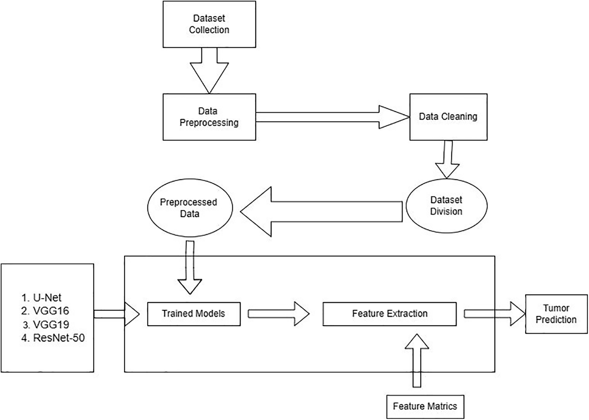
Figure 1: Workflow of the proposed work

3.1 Dataset Description

The dataset used in our proposed model was collected in TCGA (The Cancer Genome Atlas) and TCIA (The Cancer Imaging Archive). The number of identified patients from a lower grade of malignant tumors of the nervous system of TCGA was 120. Individuals had preoperative imaging data, a minimum of one containing an inversion recovery process with fluid attenuation. Ten patients were ignored in this dataset because they needed to be made aware of the available genomic constellation facts. The final group that remained in this dataset consisted of the remaining 110 patients. A detailed list of patients has been provided in Online Resource 1. The total remaining patients were divided into 22 separate, non-overlapping clusters.

Each cluster contains five patients. The process was completed for the evaluation with a cross-validation technique. The imaging dataset used in our research work was captured from Imaging Archive. Sample images with their mask are shown in Fig. 2. This dataset consists of the patients’ images related to TCGA and subsidized by the National Cancer Hospital. We used all the treatments when available, but when one was not, we only used FLAIR. Six patients lacked the pre-contrast sequence, nine lacked the post-contrast sequence, and 101 had all the relevant series. The resource has published all of the patients’ information in total 1. Among 20 to 80 patients received the number of slices. We only looked at bilateral data to detention the initial pattern of tumor progression. The genomic dataset used in this investigation included measurements of the IDH mutation 1p/19q co-deletion and DNA methylation, gene expression, DNA copy number, and microRNA expression. We consider six previously discovered genetic classifications of LGG in our research, which are known to be connected with some tumor form aspects.

•   Molecular subtype based on 1p/19q co-deletion and IDH mutation

•   4 RNA clusters

•   5 DNA methylation clusters

•   3 microRNA clusters

•   4 micro-RNA clusters

•   3 Cluster of clusters

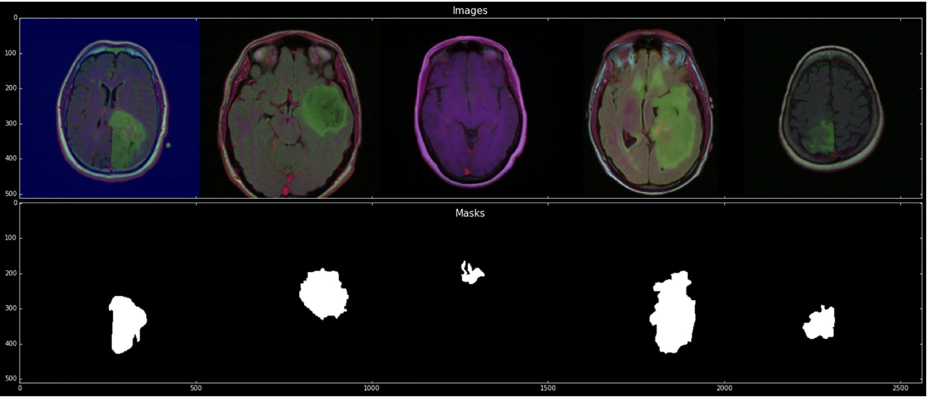
Figure 2: Sample images with mask

3.2 The U-Net Architecture

The network used by U-Net is entirely based on the network based on Convolutional layers for performing semantic segmentation tasks like fully convolutional networks (FCN) and SegNet [26–29]. U-Net architecture is based on the symmetric model with an encoder and decoder. The encoder works as an extractor of geometrical characteristics from the image. A decoder’s purpose is to build a segmentation map from encoded features. Encoders go along with the distinctive approach of CNN. It suggests a series of two 3 × 3 convolution operations, two 2 × 2 max-pooling operations, and a stride of size two followed by each. The process is repeated four times, and the number of filters doubles after each down-sampling in the convolutional layers. Finally, the Encoder and Decoder are connected by a series with two 3 × 3 convolution procedures. Alternatively, the decoder uses the 2 × 2 altered convolution procedures for up-sampling the features map, which reduces the size of the feature channel by half. An order of two 3 × 3 convolution procedures is repeated. The up-sampling and convolution procedures are repeated four times, just like with the encoder, which reduces each stage’s filter count by half. The final step involves performing a 1 × 1 convolution operation to create the segmentation map. All layers used the ReLU activation function in the pre-described model architecture by excluding the final layers for map segmentation.

The U-Net architecture uses two 3 × 3 convolutional layers in succession after each pooling layer and transposed convolutional layer. This categorization of two 3 × 3 convolutional operations looks like a 5 × 5 convolutional operation. As a result, using the Inception network’s methodology, the easiest way to provide U-Net with a multi-resolution analysis proficiency is to add 3 × 3 and 7 × 7 convolution processes in parallel to the 5 × 5 convolution operation. The model can reconcile the features learned from images at various scales when the convolution layers are replaced with blocks akin to those in Inception.

3.3 VGG-Net

A typical Convolutional neural architecture with multiple layers is called the Visual Geometry Group. A group of visual geometry at the University of Oxford develops VGGNet [30–32]. VGG 16 and VGG 19 are the most typical model of VGGNet. These models have shown tremendous success in the field of image detection. VGG-16 consists of 16 convolutional layers. It is one of the primary grounds for pattern and image recognition. The convolutional neural network known as the VGG model, which supports 16 layers, is also known as the VGG16 network. The VGG16 model achieves top-5 test accuracy of about 92.7 percent in ImageNet. About 14 million images are available in ImageNet’s collection, categorized into over 1000 categories. It was also one of the models in which the 2014 ILSVRC received the most significant interest. Sequentially substituting multiple 33 kernel-sized filters for large kernel-sized filters outperforms AlexNet. VGG network is used for our dataset adaption. As mentioned earlier, the VGGNet-16 has 16 layers and can categorize images into 1000 classes. The model also features the picture of input size 224 × 224. VGG-16 relies on the essential features of a convolutional neural network. VGG-16 consisted of tiny convolutional filters. This structure comprises 13 convolutional layers and three fully connected layers. In the VGG-16 algorithm, a max-pooling layer with a 2 × 2 kernel size follows each convolutional layer. A convolutional layer’s function is to store the training weights. Three fully connected layers are AI layers of a classifier that make up the VGG-16’s next layer. The number of parameters is determined by the fully connected layer and convolutional layers since they can store the weights of training results.

The convolutional layers used by VGG-16 have a small receptive field (3 × 3), the smallest size that still effectively catches left-right and up-down movement. In addition, the input is linearly transformed using 11 convolution filters. The ReLU unit is another key AlexNet innovation that dramatically cuts training time. A piecewise linear function called the rectified linear unit activation function (ReLU) outputs zero if the input is negative. To maintain spatial resolution after convolution, the convolution stride is set at 1 pixel (stride is the number of pixels that shifts over the input matrix). All the VGG network’s hidden layers employ ReLU. Local Response Normalization (LRN), which lengthens training and memory requirements, is hardly used in VGG. Additionally, it has no impact on total accuracy. The VGG-16 is composed of three layers. There are 4096 channels in the first two layers and 1000 channels in the third layer, one for each class.

The 16 layers of a deep neural network are represented by the number 16 in the name VGG (VGG-16). VGG16 is a massive network with approximately 138 million parameters, according to this. It is a vast network, even by today’s standards. The VGGNet16’s architecture, on the other hand, is intriguing because of its simplicity. Its architecture is highly uniform simply looking at it. After a few convolution layers, the image is pooled to reduce the image height and width. Regarding the possible filter combinations, we have about 64 options, which we may increase to about 128 and 256. We can utilize 512 filters in the final levels. The VGG-19 concept is the same as that of the VGG-16 but with a difference in the convolutional layers, as VGG-19 got 19 weighted convolutional layers compared to the 16 layers of VGG-16. VGG-19 can be trained with more than a million images from the imageNet database, and it is a deeper network that can classify images into 1000 objects.

3.4 ResNet-50

ResNet-50 was the first Residual network introduced [33–35]. It was created to add shortcut links to transform a simple network into a residual network. ResNet-50 is a deep CNN model with 50 layers. An RN Network is a network comprising a stack of blocks from artificial neural networks stacked on top of one another. This model was quite effective, as seen by the fact that its ensemble won the ILSVRC 2015 classification competition with an error rate of just 3.57 percent.

Additionally, it took first place for ImageNet detection, ImageNet localization, COCO detection, and COCO segmentation in the 2015 ILSVRC and COCO competitions. There are several different versions of ResNet, each with a different number of layers. A variant that can operate with 50 neural network layers is known as ResNet-50.

The initial experiments were implemented using different models like ResNet101, DenseNet, ShuffleNet, etc. In this study, Resnet101 shows the best results against other proposed networks. The convolutional networks include 3 × 3 filters, while the plain network was influenced by VGG neural networks (VGG-16, VGG-19). Adversely, ResNets have fewer filters and are less complex than VGGNets. The performance of the 50-layer ResNet is 3.8 billion FLOPs, compared to 3.6 billion FLOPs for smaller 34-layer ResNets.

Additionally, it followed two straightforward design principles: to preserve the time complexity per layer, each layer had the same number of filters for the same output feature map size, and the number of filters doubled if the output feature map size was cut in half. There were 50 weighted layers in total. IN ResNet-50 architecture, the building block is modified over the bottleneck for the concerns over time, taking in the training of layers. Three layers stack is used in it. The ResNet-50 architecture was created by swapping out each of the Resnet 34’s 2-layer blocks with a 3-layer bottleneck block.

4  Result

This section covers the details of our findings. We have used python as a scripting language with the following libraries: os, NumPy, pandas, matplotlib, seaborn, zip file, cv2, skimage, TensorFlow, TensorFlow Keras, random, glob, and sklearn preprocessing. These libraries helped us in data preprocessing, model training, and testing. There are two classes in the dataset: No Tumor and Tumor, with 2556 and 1337 images. The dataset was divided into training, validation, and testing with 70%, 15%, and 15%, respectively. Image data generator (IDG) generates tensors of training, testing, and validation folders. IDG parameters consist of target size (256, 256), class mode (categorial), shuffle (true), shuffle (false) only for the test folder, and batch size (16). Pretrained and integrated models take an input shape (256, 256, 3) with Adam optimizer and a learning rate of le-3 in 25 epochs. IDG parameters feed into proposed models for the required results. Several performance parameters are involved in the proposed models to understand consequences better. Training and validation loss of pre-trained and integrated pre-trained models results are shown in Fig. 3. These parameters have been listed below:

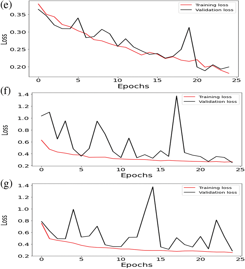
Figure 3: Training loss and validation loss of (a) ResNet-50 (b) U-Net (c) VGG16 (d) VGG19 (e) U-Net with ResNet-50 (f) U-Net with VGG16 (g) U-Net with VGG19

Accuracy: Regarding machines, learning accuracy is the correct data classification against any input or dataset. This is the measurement used to define which model is best for the pattern identification between the dataset variables of a dataset.

Validation Accuracy: Validation accuracy is also known as testing accuracy. Validation accuracy is not the accuracy that is calculated by applying the ML model to the training dataset. However, this accuracy is calculated after applying the ML model to the testing dataset.

Loss: Loss in machine learning is a number that predicts how an ML model makes many wrong predictions. If the model makes the correct prediction, the loss value remains 0. If the predictions are inaccurate, the loss value will exceed 0. The aim of training a model is to find a set of weights and biases that, on average, have low loss across all examples.

Validation Loss: A matrix called “validation loss” is used to evaluate how well the model performed on the validation data. The validation loss will be zero if a model predicts the future perfectly and more than zero if the model does not.

Dice Coefficient: The IoU and the Dice coefficient are similar. They are positively associated; thus, if one claims that model A is superior to model B at image segmentation, the other will also claim the same. They range from 0 to 1, with 1 denoting the highest resemblance between expected and truth, akin to the IoU. It is a statistical validation parameter to assess the performance of automated probabilistic fractional segmentation of MR images and the reproducibility of manual segmentations about spatial overlap accuracy. Intersection over Union: An evaluation metric called intersection over union assesses an object detector’s precision on a specific dataset.

Dice Coefficient Loss: The dice coefficient is a popular statistic for determining how similar two images are in computer vision.

Jaccard Distance: The Jac- card Index, often known as the Jaccard similarity coefficient, is a statistic used to analyze the similarities between sample sets. Formally speaking, the measurement is the size of the intersection divided by the size of the union of the sample sets and emphasizes the similarity between finite sample sets. The Jaccard distance gauges the dissimilarity between sample sets, much as the Jaccard Index, which measures similarity. Finding the Jaccard index and deducting it from one or dividing the differences by the intersection of the two sets yields the Jaccard distance.

Mean: A dataset’s mean is calculated by dividing the total values by the sum of all the values. It is sometimes called the “average” and is the most widely used central tendency metric.

Standard Deviation: One of the most important ways to evaluate a machine learning model’s correctness concerning actual data is to use this metric to determine the variability of a population or sample. Standard deviation can also be used to gauge how confident one is in a model’s statistical findings.

25th Percentile: The first or lower quartile is often called the 25th percentile. The value at which 25% of the answers fall below it and 75% of the responses fall above it is known as the 25th percentile.

50th Percentile: The 50th percentile is also referred to as the median. The data set is divided in half by the median. Half of the responses fall below the median, while the other half rise beyond.

75th Percentile: The third or higher quartile is another name for the 75th percentile. The value at which 25% of the answers are above that value, and 75% below that value is known as the 75th percentile. As explained earlier, different criteria for evaluating the ML model performance exist. Accuracy plays an essential role in the version of a model. Our proposed approach uses different machine learning algorithms to assess the model’s performance. Different algorithms show different results, as explained below.

4.1 Pre-Trained ResNet-50 Model

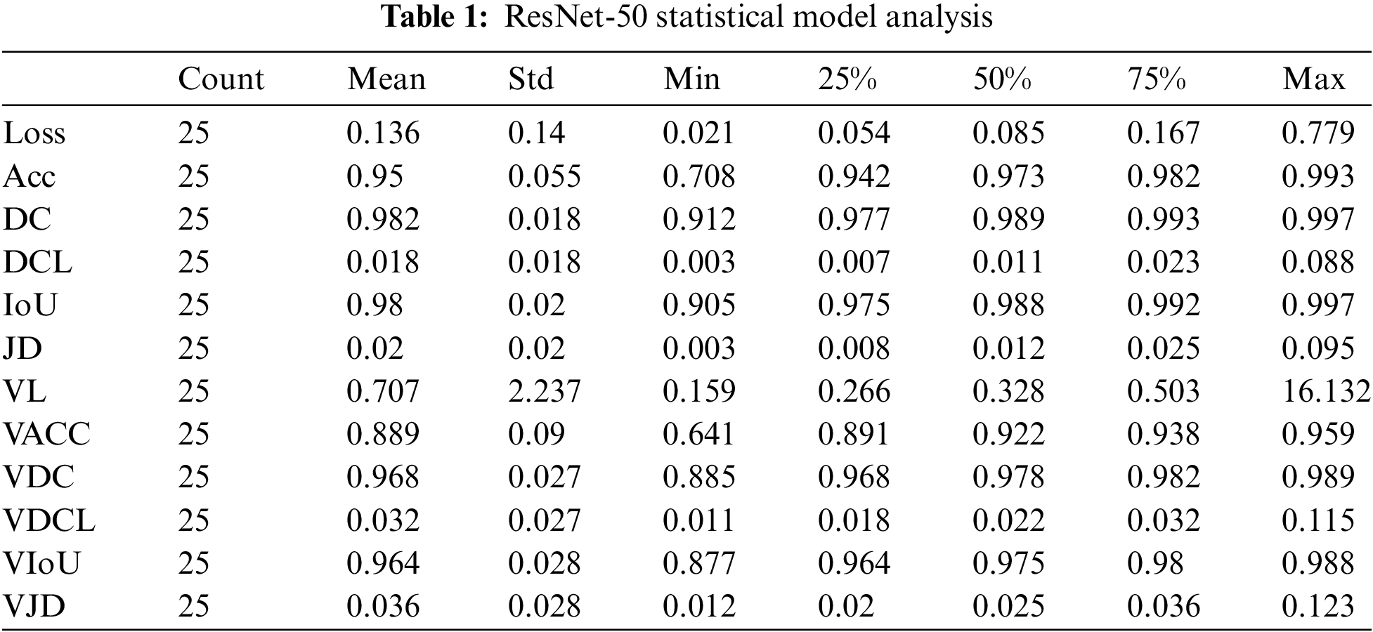
Concerning 25 epochs, the ResNet-50 algorithm offers us roughly 95 percent validation and 99 percent training accuracy. The maximum Dice coefficient loss during training was 0.01, and the maximum Dice coefficient loss during validation was approximately 0.02. About 99 percent of the union was gained throughout training and 98 percent during validation. The Dice coefficient was almost 99 percent during training and 98 percent during validation. Jaccard’s distance was roughly 0.02 during validation and 0.01 during training. During training, the loss was equal to 0; during validation, it was approximately 0.01.

The number of epochs utilized to train our ResNet-50 model, Count, is displayed in Table 1 for reference. The mean value fluctuates concerning other factors from 0.01 to 0.98. The value of the standard deviation ranges from 0.01 to 2.23. The 25th percentile’s value might vary from 0.006 to 0.97. The 50th percentile’s weight ranges from 0.01 to 0.989. The value of the 75th percentile ranges from 0.02 to 0.99. The maximum parameter factor ranges from 0.11 to 16.13.

4.2 Pre-Trained U-Net Model

Regarding accuracy, the U-Net method offers us 25 epochs of training and validation data with an accuracy of almost 100% in both cases. The maximum Dice coefficient loss during training was −0.7; during validation, it was roughly 0.65. The difference between union gains made during training and validation was approximately 66 percent and 55 percent, respectively. Between training and validation, the Dice coefficient varied between 65 and about 80 percent. Jaccard’s distance was −0.6 during training and about −0.55 during validation. A loss of about −0.7 was experienced during training, while about −0.65 was experienced during validation.

According to Table 2, Count is the number of epochs used to train our U-Net model. The mean value varies to other factors from −0.6 to 0.99. The value of the standard deviation ranges from 0.009 to 0.16. The 25th percentile’s value is from −0.7 to 0.99. The 50th percentile’s weight ranges from 0.66 to 0.99. The range of the 75th percentile value is from −0.57 to 0.99. The maximum parameter value ranges from −0.2 to 0.99.

4.3 Pre-Trained VGG16 Model

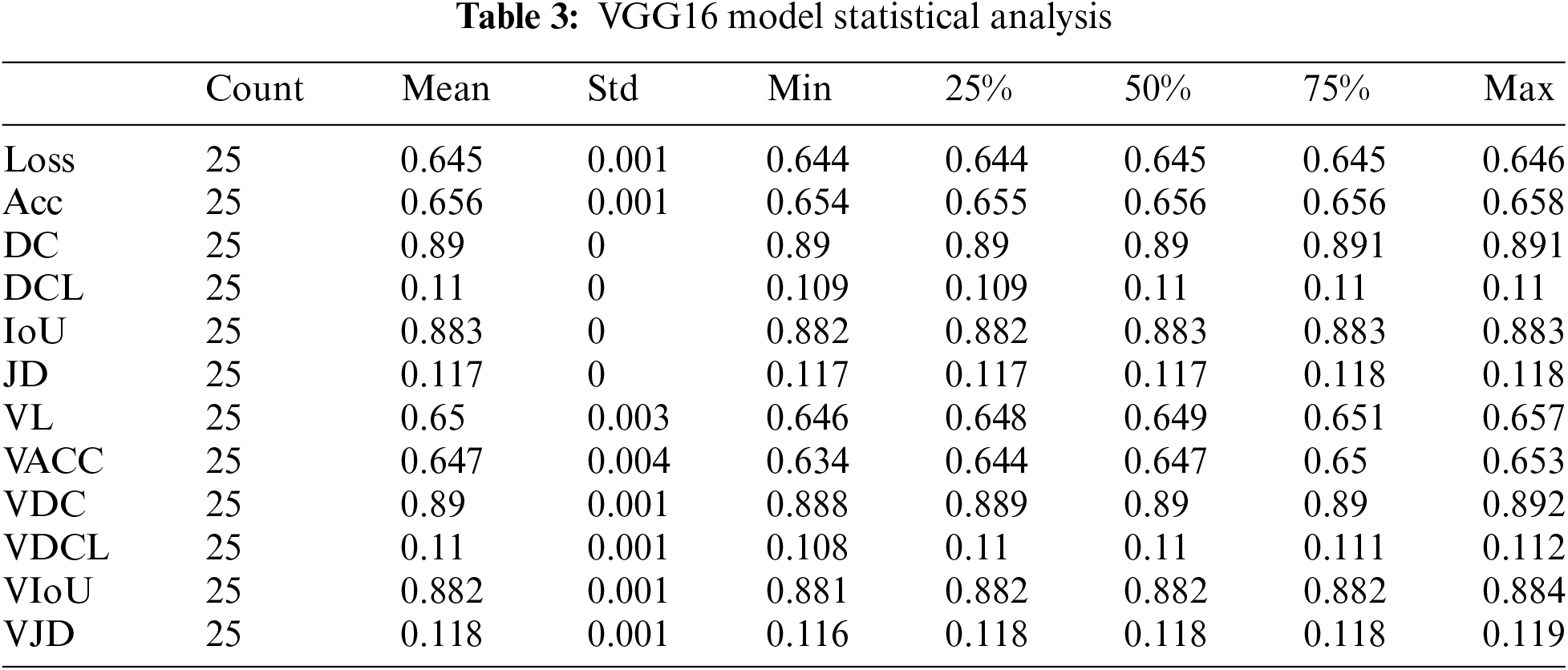
The VGG 16 algorithm gives us approximately 65.5 percent training accuracy and 65 percent validation accuracy for 25 epochs. The maximum dice coefficient loss during training was 0.1100; during validation, the most significant loss was around 0.1095. The union increased by about 88 percent during training and 88 percent during validation. The Dice coefficient was approximately 89 percent during training and 89.5 percent during validation. The Jaccard distance was 0.1175 during training and around 0.1173 during validation. The loss was equal to 0.644 during training and approximately 0.646 during validation.

According to Table 3, Count is the number of epochs used to train our VGG16 model. The mean value varies with other parameters from 0.10 to 0.89. The value of the standard deviation ranges from 0.00035 to 0.0044. The 25th percentile’s value might range from 0.10 to 0.89. The 50th percentile’s weight ranges from 0.10 to 0.89. The range of the 75th percentile value is 0.10 to 0.89. The maximum parameter value ranges from 0.11 to 0.89.

4.4 Pre-Trained VGG19 Model

VGG 19 algorithm provides us approximately 65.5% training accuracy and about 64.3% validation accuracy against 25 epochs. The maximum dice coefficient loss gained during the training was 0.890, and the validation dice coefficient loss was approximately 0.89. Intersection over union gained during training was about 0.883, and during validation was 0.882. The Dice Coefficient during training was appr 0.109, and during validation was 0.110. The value of Jaccard distance during training was 0.1175 and, during validation, was appr 0.118. The loss value during training was 0.644, and during validation was appr 0.66.

According to Table 4. the Count is the number of epochs used to train our VGG19 model. The mean value varies with other parameters from 0.10 to 0.89. The value of the standard deviation ranges from 0.0005 to 0.005. The 25th percentile’s value might range from 0.10 to 0.89. The 50th percentile’s weight ranges from 0.10 to 0.89. The range of the 75th percentile value is 0.10 to 0.89. The maximum parameter value ranges from 0.11 to 0.89.

4.5 Integration of U-Net with ResNet-50

Integrating U-Net with ResNet-50, the Dice Coefficient for testing was 90% and 80% for validation data by applying 25 epochs. The dice coefficient loss gained during training was −0.90, and during validation, the loss was −0.85. The value of testing intersection over union was 0.80, and validation IoU was 0.68. The Testing Jaccard distance value was −0.75, and the validation Jaccard distance was −0.68. The loss value for testing data was 0.18; for validation, the loss was 0.22.

The results count from integrating the U-Net with ResNet-50 is displayed in Table 5—the mean value changes to other parameters between −0.75 and 0.75. The value of the standard deviation ranges from 0.04 to 0.061. The 25th percentile’s score can go from −0.79 to 0.71. The 50th percentile’s weight ranges from −0.76 to 0.76. The value of the 75th percentile ranges from −0.71 to 0.79. The maximum parameter value ranges from −0.63 to 0.82.

4.6 Integration of U-Net with VGG16

As U-Net was integrated with VGG16, the gained testing Dice Coefficient was 73%, and the validation Dice Coefficient was 75% by applying 25 epochs.

Training Dice coefficient loss was 0.7, and the validation dice coefficient loss was −0.72. The value of testing intersection over union was 0.6, and validation IoU was 0.64. The Testing Jaccard distance value was −0.6, and the validation Jaccard distance was −0.63. The loss value for testing data was 0.3, and for validation, the loss was 0.3.

The results count from integrating the U-Net with VGG16 is displayed in Table 6. The mean value fluctuates about other factors from −0.68 to 0.68. The value of the standard deviation ranges from 0.08 to 0.30. The 25th percentile’s score might go from −0.73 to 0.67. The 50th percentile’s weight ranges from −0.71 to 0.71. The value of the 75th percentile ranges from −0.67 to 0.73. The maximum parameter value ranges from −0.39 to 1.37.

4.7 Integration of U-Net with VGG19

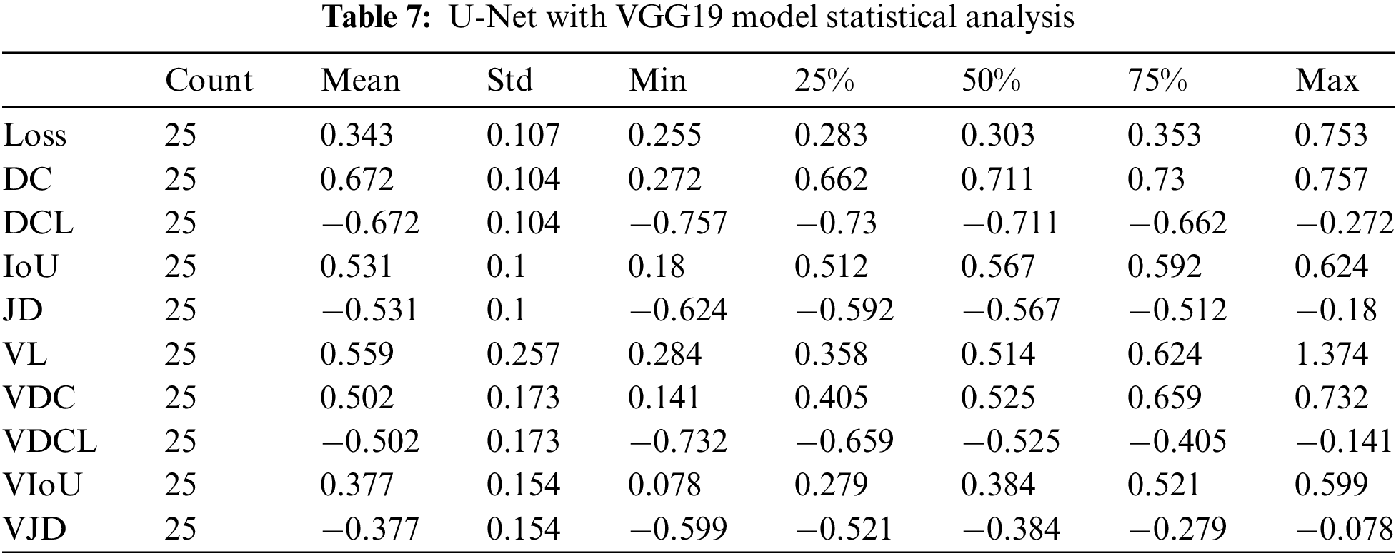
In applying integration on U-Net with VGG19, we gained 75% Dice Coefficient accuracy and 70% validation Dice Coefficient using 25 epochs. The dice coefficient loss was 0.75, and the validation dice coefficient loss was −0.7. The value of testing intersection over union was 0.60, and validation IoU was 0.58. The Testing Jaccard distance value was −0.6, and the validation Jaccard distance was −0.58. The loss value for testing data was 0.27, and for validation, the loss was 0.3.

The results count from integrating the U-Net with VGG19 is displayed in Table 7. The mean value fluctuates to other factors from −0.68 to 0.68. The value of the standard deviation ranges from 0.08 to 0.30. The 25th percentile’s score might go from −0.73 to 0.67. The 50th percentile’s weight ranges from −0.71 to 0.71. The value of the 75th percentile ranges from −0.67 to 0.73. The maximum parameter value ranges from −0.39 to 1.37.

5  Discussion

According to the above study, brain tumors are currently regarded as one of the leading causes of death in children and adults. A scale from grade I to grade IV is employed, by World Health Organization (WHO) and American Brain Tumor Association, to distinguish between benign and malignant tumor forms. Machine learning techniques are utilized to classify cancer detection studies because they excel in image analysis, including image classification, object recognition, and semantic segmentation. For the category of brain tumors, we have used the U-Net, VGG Net, and ResNet-50 architecture in the suggested study. U-Net is particularly well-suited for image segmentation tasks because it can accurately locate and segment small objects in images and handle images with varying shapes and sizes. It has been used in several medical imaging applications, such as segmenting tumors in MRI images and identifying cells in microscopic images.

Instead of employing enormous fields like AlexNet, VGG Net used small receptive fields like 3 × 3 with a stride of 1. VGG Net has many parameters, making it a powerful model, but it also requires a large amount of memory and computational power to train and use. Despite this limitation, VGG Net has been widely used as a base model for our computer vision tasks, such as object detection and semantic segmentation.

Additionally, ResNet-50 was utilized for training many images while maintaining a low error rate. ResNet-50 has been trained on the ImageNet dataset and achieved state-of-the-art image classification results. Due to its good performance and relative simplicity, it has been widely used as a base model for many computer vision tasks, such as object detection and semantic segmentation. The data for our suggested model was gathered from the TCIA (The Cancer Imaging Archive) and TCGA (The Cancer Genome Atlas). The TCIA and TCGA data is a valuable resource for researchers in the field of cancer genomics, enabling them to use large amounts of data to identify new cancer-causing genes, understand the mechanisms of cancer development, and identify new targets for cancer therapy. The data is also used to develop and evaluate cancer diagnosis and prognosis computational models. One hundred one patients had all the necessary sequences, while six were missing the pre-contrast series, and nine were missing the post-contrast series.

Applying several techniques to available dataset during this study yields impressive results. The training and validation accuracy of pre-trained algorithms like ResNet-50, U-Net, VGG16, and VGG19 is excellent.

The results presented in Tables 1–7 are summary of 12 different metrics for a machine learning model on a validation set, each with 25 observations. The metrics include loss, accuracy, Dice coefficient, Jaccard distance, and intersection over union, among others. For each metric, the table shows the count, mean, standard deviation, minimum, 25th percentile, median, 75th percentile, and maximum values across the 25 observations. The mean values provide an indication of the performance of the machine learning model on the validation set, while the standard deviation shows the degree of variability across the observations. The minimum and maximum values highlight the range of possible values for each metric, while the percentiles give an idea of the distribution of the observations. Overall, the tables provide a comprehensive overview of the performance of the machine learning model on the validation set across different evaluation metrics.

In term of loss, ResNet-50 achieved lowest values 0.136 whereas VGG19 has higher loss value 0.648. In term of accuracy, U-Net got 99% correct classification while VGG16 and VGG19 performed worst by obtaining 65% accuracy. In term of dice coefficient, ResNet-50 works exponentially and achieved 98% correct results and U-Net performs worst by taking only 62% correct values. The dice coefficient loss ranges from 0 to 1, therefore we have not considered negative values. The lowest dice coefficient loss values in our proposed study is 0.018 which is claimed by ResNet-50 and higher value 0.11 achieved by VGG16 and VGG19.

In the context of intersection over union, ResNet-50 attained 98% of the predicted region overlaps while U-Net gets only 48.5%. The Jaccard distance ranges from 0 to 1, where a score of 0 indicates that the two sets are identical, and a score of 1 indicates that the two sets have no elements in common. In term of Jaccard distance, highest 0.02 and lowest 0.11 values were obtained by ResNet-50 and VGG 16 respectively. During validation loss, U-Net with ResNet-50 model achieved lowest loss 0.267 while ResNet-50 faces higher loss 0.707 as compared to other models. U-Net and VGG16 provide validation accuracy 99% highest and 64.7% lowest respectively as compared to proposed algorithms. In term of validation dice coefficient, highest and lowest values accomplished through ResNet-50 and U-Net with VGG19.

As per validation dice coefficient loss, lowest value 0.032 and highest value 0.11 achieved by ResNet-50 and VGG19. In validation Intersection over union, ResNet-50 achieved higher values while U-Net with VGG19 got lowest value 96% and 37% respectively. In term of validation Jaccard distance, ResNet-50 performs better and VGG19 achieve lowest value 0.036 and 0.11 respectively.

The suggested approach extracted data from images of glioma tumors using the principles of numerous deep-learning techniques. The features were employed with various tested, trained, and integrated models for better performance.

6  Conclusion

This study proposes a precise and automatic technique for classifying brain tumors using various advanced algorithms. The proposed system used the idea of several deep-learning techniques to extract information from photos of glioma tumors. For better performance, the extracted characteristics were used with multiple tested, trained, and integrated models. The system’s classification accuracy with the suggested algorithm was the best compared to all the similar works. Our proposed method also integrated U-Net with other algorithms to assess the system’s performance. The accuracy provided by the pre-trained U-Net model has higher than others. Higher performance was achieved from the integration of U-Net with ResNet-50 on the dataset. Parameters like mean, std, min, max, 25th percentile, 50th percentile, and 75th percentile were also counted. The proposed system used a dataset of brain scans from cancer patients to train and evaluate the algorithm’s performance. The dataset was collected from various medical institutions and preprocessed to remove irrelevant information. The system was tested on a separate dataset to evaluate its performance. The results showed that the proposed method accurately classified brain tumors. The system correctly identified the type of brain tumor with an accuracy of more than 95%. This high level of accuracy is a significant improvement over the existing methods and could lead to more accurate diagnosis and treatment of brain tumors. In addition to the classification performance, the proposed system has a user-friendly interface that allows radiologists and medical professionals to use the system for diagnostic purposes easily. The system can be integrated into existing radiology systems and assist radiologists in diagnosing brain tumors. Overall, the proposed method demonstrates the potential of using advanced deep learning techniques and integrating U-Net with other algorithms to classify brain tumors accurately. The system’s high accuracy and user-friendly interface make it a valuable tool for diagnosing and treating brain tumors.

Acknowledgement: The authors acknowledge the support from the Deanship of Scientific Research, Najran University. Kingdom of Saudi Arabia, for funding this work under the Distinguish Research funding program Grant code Number (NU/DRP/SERC/12/7).

Funding Statement: This research was supported by the Deanship of Scientific Research, Najran University. Kingdom of Saudi Arabia, Project Number (NU/DRP/SERC/12/7).

Availability of Data and Materials: Dataset can be downloaded from the given link: https://wiki.cancerimagingarchive.net/display/Public/TCGA-LGG.

Conflicts of Interest: The authors declare that they have no conflicts of interest to report regarding the present study.

References

1. “Brain Tumors Classifications, Symptoms, Diagnosis and Treatments,” [Online]. Available: https://www.aans.org/Patients/Neurosurgical-Conditions-and-Treatments/Brain-Tumors. [Accessed 20 April 2022]. [Google Scholar]

2. “Brain Tumor: Introduction—Cancer.Net.,” [Online]. Available: https://www.cancer.net/cancer-types/brain-tumor/introduction. [Accessed 20 April 2022]. [Google Scholar]

3. [Online]. Available: https://www.abta.org/about-brain-tumors/brain-tumor-education/. [Accessed 20 April 2022]. [Google Scholar]

4. S. Abbasi and F. Tajeripour, “Detection of brain tumor in 3D MRI images using local binary patterns and histogram orientation gradient,” Neurocomputing, vol. 219, no. 3, pp. 526–535, 2017. [Google Scholar]

5. P. Kleihues, P. C. Burger and B. W. Scheithauer, “The new WHO classification of brain tumours,” Brain Pathology, vol. 3, no. 3, pp. 255–268, 1993. [Google Scholar] [PubMed]

6. N. Singh and A. Jindal, “Ultra sonogram images for thyroid segmentation and texture classification in diagnosis of malignant (cancerous) or benign (non-cancerous) nodules,” International Journal of Engineering Innovation Technology, vol. 1, no. 1, pp. 202–206, 2012. [Google Scholar]

7. N. B. Bahadure, A. K. Ray and H. P. Thethi, “Image analysis for MRI based brain tumor detection and feature extraction using biologically inspired BWT and SVM,” International Journal of Biomedical Imaging, vol. 2017, no. 3, pp. 1–13, 2017. [Google Scholar]

8. S. Bauer, R. Wiest, L. -P. Nolte and M. Reyes, “A survey of MRI-based medical image analysis for brain tumor studies,” Physics Medical Biology, vol. 58, no. 13, pp. 97–129, 2013. [Google Scholar]

9. S. Ruan, S. Lebonvallet, A. Merabet and J. -M. Constans, “Tumor segmentation from a multispectral MRI images by using support vector machine classification,” in Proc. 2007 4th IEEE Int. Symp. on Biomedical Imaging: From Nano to Macro, Arlington, VA, USA, pp. 1–4, 2007. [Google Scholar]

10. S. K. Mishra and V. H. Deepthi, “Brain image classification using dual tree M-band wavelet transforms and support vector machine,” Indian Journal of Public Health Research and Development, vol. 10, no. 11, pp. 3845–3849, 2019. [Google Scholar]

11. S. Reza and K. Iftekharuddin, “Multi-class abnormal brain tissue segmentation using texture,” Multimodal Brain Tumor Segmentation, vol. 38, no. 2, pp. 38–42, 2013. [Google Scholar]

12. A. Krizhevsky, I. Sutskever and G. E. Hinton, “ImageNet classification with deep convolutional neural networks,” Communication ACM, vol. 60, no. 6, pp. 84–90, 2017. [Google Scholar]

13. S. Abbasi, “Ultra sonogram images for thyroid segmentation and texture classification in diagnosis of malignant (cancerous) or benign (non-cancerous) nodules detection of brain tumor in 3D MRI images using local binary patterns and histogram orientation gradient,” International Journal of Engineering Innovation and Technology, vol. 219, no. 2, pp. 84–90, 2007. [Google Scholar]

14. Z. Liu, X. Li, P. Luo, C. -C. Loy and X. Tang, “Semantic image segmentation via deep parsing network,” in Proc. 2015 IEEE Int. Conf. on Computer Vision (ICCV), Santiago, Chile, pp. 1377–1385, 2015. [Google Scholar]

15. J. Kang, Z. Ullah and J. Gwak, “MRI-based brain tumor classification using ensemble of deep features and machine learning classifiers,” Sensors (Basel), vol. 21, no. 6, pp. 2222–2243, 2021. [Google Scholar] [PubMed]

16. R. Wang, “AdaBoost for feature selection, classification and its relation with SVM, A review,” Physics Procedia, vol. 25, no. 4, pp. 800–807, 2012. [Google Scholar]

17. J. Guo and X. Wang, “Image classification based on SURF and KNN,” in Proc., 2019 IEEE/ACIS 18th Int. Conf. on Computer and Information Science (ICIS), Beijing, China, pp. 1–4, 2019. [Google Scholar]

18. K. Simonyan and A. Zisserman, “Very deep convolutional networks for large-scale image recognition,” arXiv [cs.CV], 2014. [Google Scholar]

19. K. He, X. Zhang, S. Ren and J. Sun, “Deep residual learning for image recognition,” in Proc., 2016 IEEE Conf. on Computer Vision and Pattern Recognition (CVPR), Las Vegas, NV, USA, pp. 770–778, 2016. [Google Scholar]

20. A. Maruthamuthu and L. P. Gnanapandithan G., “Brain tumour segmentation from MRI using superpixels based spectral clustering,” Journal of King Saud University – Computer and Information Science, vol. 32, no. 10, pp. 1182–1193, 2020. [Google Scholar]

21. C. J. J. Sheela and G. Suganthi, “Automatic brain tumor segmentation from MRI using greedy snake model and fuzzy C-means optimization,” Journal of King Saud University – Computer and Information Science, vol. 34, no. 3, pp. 557–566, 2022. [Google Scholar]

22. K. S. Ananda Kumar, A. Y. Prasad and J. Metan, “A hybrid deep CNN-cov-19-res-net transfer learning architype for an enhanced brain tumor detection and classification scheme in medical image processing,” Biomedical Signal Processing and Control, vol. 76, no. 103631, pp. 1–16, 2022. [Google Scholar]

23. A. S. Akbar, C. Fatichah and N. Suciati, “Single level UNet3D with multipath residual attention block for brain tumor segmentation,” Journal of King Saud University – Computer and Information Science, vol. 34, no. 6, pp. 3247–3258, 2022. [Google Scholar]

24. P. Wang and A. C. S. Chung, “Relax and focus on brain tumor segmentation,” Medical Image Analyzing, vol. 75, no. 1, pp. 102259–102274, 2022. [Google Scholar]

25. A. A. Asiri, “A novel inherited modeling structure of automatic brain tumor segmentation from MRI,”Computers, Materials & Continua, vol. 73, no. 2, pp. 3983–4002, 2022. [Google Scholar]

26. U. Ilhan and A. Ilhan, “Brain tumor segmentation based on a new threshold approach,” Procedia Computing Science, vol. 120, no. 3, pp. 580–587, 2017. [Google Scholar]

27. F. Li, Z. Long, P. He, X. Guo, X. Ren et al., “Fully convolutional pyramidal networks for semantic segmentation,” IEEE Access, vol. 8, no. 2, pp. 229132–229140, 2020. [Google Scholar]

28. Y. Nakayama, H. Lu, Y. Li and T. Kamiya, “Widesegnext: Semantic image segmentation using wide residual network and NeXt dilated unit,” IEEE Sensor Journals, vol. 21, no. 10, pp. 11427–11434, 2021. [Google Scholar]

29. M. D. Zeiler, G. W. Taylor and R. Fergus, “Adaptive deconvolutional networks for mid and high level feature learning,” in Proc. 2011 Int. Conf. on Computer Vision, Barcelona, Spain, pp. 1–4, 2011. [Google Scholar]

30. Y. Matsuo, Y. LeCun, M. Sahani, D. Precup, D. Silver et al., “Deep learning, reinforcement learning, and world models,” Neural Networks, vol. 152, no. 4, pp. 267–275, 2022. [Google Scholar] [PubMed]

31. M. Drozdzal, E. Vorontsov, G. Chartrand, S. Kadoury and C. Pal, “The importance of skip connections in biomedical image segmentation,” in Proc. Deep Learning and Data Labeling for Medical Applications, Cham: Springer Int. Publishing, Athens, Greece, pp. 179–187, 2016. [Google Scholar]

32. A. Garcia-Garcia, S. Orts-Escolano, S. Oprea, V. Villena-Martinez and J. Garcia-Rodriguez, “A review on deep learning techniques applied to semantic segmentation,” arXiv [cs.CV], 2017. [Google Scholar]

33. H. Eghbal-Zadeh, B. Lehner, M. Dorfer and G. Widmer, “CP-JKU submissions for DCASE-2016: A hybrid approach using binaural i-vectors and deep convolutional neural networks,” IEEE AASP Challenge on Detection and Classification of Acoustic Scenes and Events (DCASE), vol. 6, no. 2, pp. 5024–5028, 2016. [Google Scholar]

34. K. He, X. Zhang, S. Ren and J. Sun, “Deep residual learning for image recognition,” arXiv [cs.CV], 2015. [Google Scholar]

35. R. Roslidar, K. Saddami, F. Arnia, M. Syukri and K. Munadi, “A study of fine-tuning CNN models based on thermal imaging for breast cancer classification,” in Proc. 2019 IEEE Int. Conf. on Cybernetics and Computational Intelligence (CyberneticsCom), Banda Aceh, Indonesia, pp. 1–4, 2019. [Google Scholar]