Fault Diagnosis of Power Electronic Circuits Based on Adaptive Simulated Annealing Particle Swarm Optimization

1  Introduction

With the continuing development and improvement of power electronic devices, how to achieve high energy efficiency is attracting increasing attention. Power electronic converters are vital devices in energy conversion. They have a high power and high current characteristic. They can balance the grid and play an essential role in energy conversions, such as energy generation and transmission, transportation, and hybrid electric vehicles [1,2]. The reliability of power electronic circuits plays a crucial role in the stable operation of the energy system. If an abnormality occurs in a power electronic circuit, the equipment can become damaged, or the entire energy system may become paralyzed. Thus, it is essential to study how to diagnose faults [3,4].

When a fault occurs in a power electronic circuit, the fault information is present only briefly after the occurrence of the fault and before the outage. Therefore, real-time dynamic monitoring and online diagnosis are required. According to the different characteristics of fault diagnosis methods, there are three main methods for diagnosing faults in a power electronic circuit: mathematical modeling, signal processing, and knowledge analysis [5–7].

A mathematical model can visualize the changes in the state variables. However, it isn’t easy to obtain a mathematical model that is sufficiently accurate due to the nonlinearity of power electronic circuits [8,9]. Mathematical models commonly used for diagnosis are state estimation, parameter estimation, and equivalent space estimation. An accurate mathematical model is not required for diagnosis based on signal processing. Researchers can determine the location of a fault from the relation between the post-fault and system results. However, due to the complex structure of power electronic circuits, the fault characteristics in acquired signals are sometimes not prominent, and it cannot be easy to extract useful information [10]. Signal processing methods commonly used for diagnosis are spectrum analysis, wavelet transforms, and signal fusion.

Knowledge-based methods are efficient and less dependent on the circuit model than the previous two methods. They utilize only historical data and have a high adaptive and memory capacity. A knowledge-based process does not require an exact and sophisticated mathematical model. Moreover, it does not need to analyze signal patterns [11,12]. Therefore, this approach is currently the most commonly used method for diagnosing and analyzing faults in power electronic circuits. Over the past few years, neural networks have been widely used for diagnosing faults in power electronic circuits [13,14]. To analyze different fault modes, a method with a Bayesian network (BN) has been proposed [15]. Feature information was extracted from the line voltage of the input signal by Fourier analysis. Feature samples were dimensioned down using principal component analysis (PCA). The results were input to a Bayesian network, which diagnosed different fault modes. A diagnostic method with a support vector machine (SVM) and PCA has also been presented [16]. The diagnostic object of this method was a three-phase rectifier, which selects the output voltage signal for analysis. PCA was used to extract various fault features, and the fault type was classified with SVM. A fault classification algorithm for inverters based on an SVM has been proposed [17]. The classification and localization of open-circuit faults in insulated gate bipolar transistors in inverters are achieved using a vector machine. An open-circuit fault diagnosis method with an intelligent optimization algorithm has been developed [18]. The way detects and extracts fault features with a discrete wavelet transform (DWT) and PCA. The detection algorithm used in this method is a two-sample technique, and the feature location algorithm selected is wavelet packet entropy. A fuzzy logic system (FLC) and a correlation vector machine (RVM) were employed for fault classification. Based on this, it combines Evolutionary Particle Swarm Optimisation (EPSO) and Cuckoo Search Optimisation algorithms to improve fault diagnosis. The experimental results showed that combining cuckoo search optimization and a correlation vector machine can perform better. It is important to note that diagnosing faults in power electronic circuits is a typical feature-classification problem. Thus, an optimization method based on an extensive feedforward network with self-adaptive parameters and a strategy-based particle swarm algorithm has been proposed [19]. Features were selected from a large dataset. The weights of an extensive feedforward network were optimized using this algorithm, which improved classification accuracy and reduced the calculation complexity. An algorithm to introduce an adaptive strategy in multi-objective PSO has been proposed [20]. It uses decomposition methods with punitive boundary interactions to find the best solution. It gives a different penalty value to each weight vector, and this adjustment is adaptive. Moreover, the method effectively identifies particles that are at the local optimum. According to the experimental results, this algorithm demonstrates strong convergence and diversity in high-dimensional data sets.

Our literature review found that every method for extracting or diagnosing fault features based on a single intelligent algorithm has limitations and shortcomings. Thus, obtaining satisfactory results with only one fault diagnosis method can be difficult. By combining multiple intelligent learning algorithms to enhance the performance of networks, the accuracy and timeliness of diagnosing faults in a power electronic circuit can be effectively improved. PSO has been widely used for combinatorial optimization problems because few parameters must be set and have computational simplicity. Many scholars have conducted a significant amount of research into optimization to solve the premature maturity and slow convergence of PSO algorithms. There are three main research directions: improving the iteration strategy, integrating with other optimization algorithms, and improving the population topology.

The iteration strategy can be improved by changing the inertia weights and learning factors of the PSO algorithm linearly or non-linearly with the number of iterations. A large two-level PSO algorithm has been presented [21]. The algorithm’s convergence was accelerated using an increasing exponential function to control the learning factor. A global PSO algorithm has also been proposed [22]. It improves the global search capability of the algorithm by introducing a cosine function to adjust the inertia weights afterward. In addition, It also solves the premature convergence problem of the particle swarm algorithm by integrating it with another optimization algorithm. For example, a hybrid algorithm combines the PSO and genetic algorithms with crossover and mutation operators [23]. This approach reduces the number of local minima. The experimental results show that the performance of a single intelligent algorithm is not as good as that of fusing several algorithms. In addition, the population topology can be enhanced by transforming the D-dimensional space into a chaotic space. The ergodic characteristics of chaos are used in the iterations. By exploiting this feature, it can significantly improve the algorithm’s overall performance. A PSO algorithm based on chaotic initialization time variation has been proposed for optimizing the parameters of a transmission line [24]. It avoids premature convergence and helps to enhance the chances of a particle jumping out of a local optimum.

In this study, we improved the previous two of the three directions. A linear change strategy controls the learning factor, a negative hyperbolic tangent function adjusts the inertia weights, and a simulated annealing (SA) algorithm integrates into the iterative process. Thus the chances of the algorithm jumping out of a local optimum are significantly increased. Therefore, this paper proposes an algorithm that employs a fusion of a network and intelligent optimization to diagnose and classify open-circuit faults in a power electronic circuit. For example, we apply the method to an open thyristor fault in a three-phase rectifier circuit. First, the characteristics of the circuit model in regular operation and mark states are analyzed. Second, the fault characteristics are extracted from a signal in a sample dataset using a Fourier transform. The results are input into a backpropagation (BP) network. The accuracy of the fault diagnosis is obtained by analyzing the actual and desired output of the network. Finally, the parameters of the BP network are optimized with the PSO algorithm and the ASAPSO algorithm, which is then used to diagnose faults. The experimental results show that the BP network optimized with the ASAPSO algorithm achieves an accuracy of 95.5% in diagnosing faults, demonstrating that fault diagnosis and localization can be performed accurately and quickly.

The rest of the paper is organized as follows. Section 2 presents the fault modes and the extraction of features from a signal for the circuit. Section 3 presents the process of a BP network for fault diagnosis. The PSO algorithm first optimizes the parameters and then the ASAPSO algorithm. Section 4 presents the experimental validation of the proposed method, which is performed in MATLAB. Our conclusions are drawn in the last section.

2  Extraction of Fault Features from a Signal

The topology of a three-phase bridge rectifier circuit is shown in Fig. 1. Where VT1, VT3, and VT5 are common cathode group thyristors, VT4, VT6, and VT2 are common anode group thyristors, R is a resistor, L is an inductor, and ud is the load output voltage. In the regular operation of the circuit, there is a thyristor in the common cathode at any moment, and a thyristor in the common anode is turned on simultaneously to form the current path. The phase is changed every π/3. In one cycle, the thyristors are turned on in a specific order, and the conduction situation is VT1 → VT2 → VT3 → VT4 → VT5 → VT6.

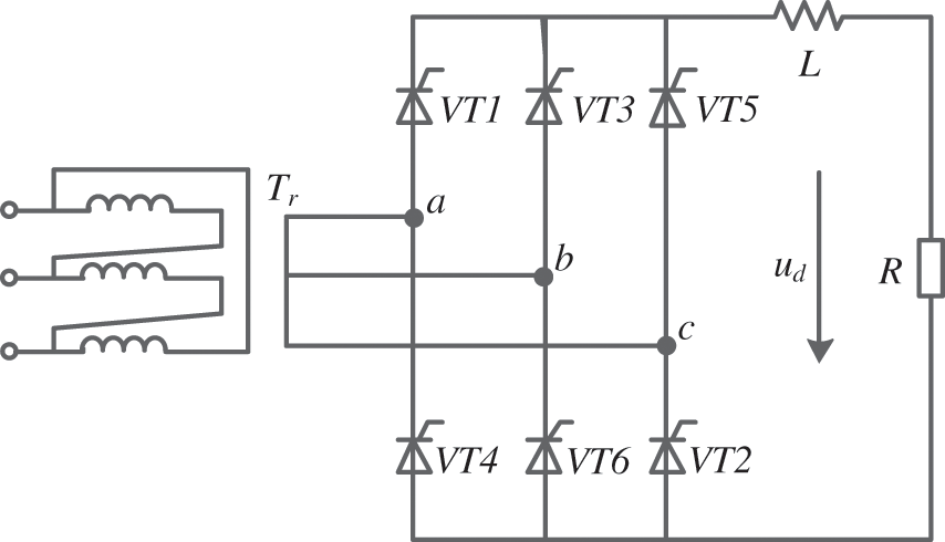
Figure 1: Three-phase bridge rectifier circuit

In actual operation, the primary faults in power electronic circuits are thyristor open and short-circuit faults [25]. To make it easier to analyze, we will only discuss single and double open circuits in this paper. We treat a normal circuit condition as a specific fault. Overall, there are C61 + C62 + 1 = 22 faults, corresponding to 22 states of the circuit, which are numbered from 1 to 22.

The output voltage ud at the load side of the rectifier bridge is not only easy to measure, but its waveform contains various fault information. Therefore, ud is chosen as the object of analysis in this paper. Voltage waveforms ud of the 22 faults were obtained by simulating an open-circuit fault at trigger angle α = 0° for each thyristor. We simulated the circuit illustrated in Fig. 1. Two typical fault waveforms are shown in Fig. 2.

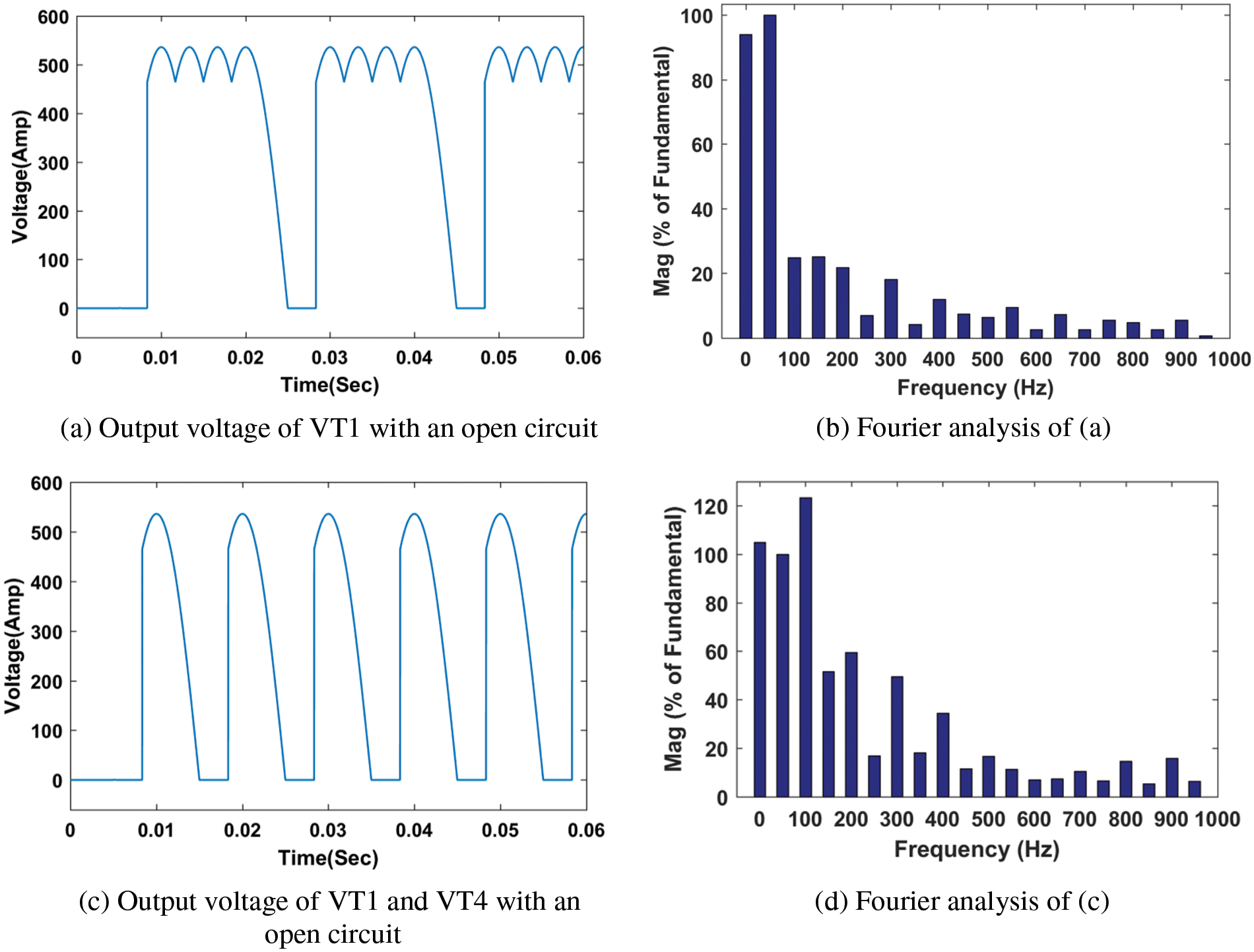
Figure 2: Output voltages and Fourier analysis of faults

The waveforms in Figs. 2a and 2c demonstrate that the ud waveforms under different fault types differ significantly for the same trigger angle α. The waveform shapes for different faults of the same type are shifted along the time axis. When the trigger angle α changes, the shape of the ud waveform will correspondingly change. The Fourier analysis in Figs. 2b and 2d show that the features needed for fault diagnosis are contained in the former third harmonic of ud. Therefore, the DC component a0 and previous third harmonic amplitudes A1, A2, and A3 of ud are selected as containing information about fault features. Before inputting into the neural network, the data were normalized to reduce the computation required to process it.

3  Proposed Methodology

3.1 Fault Diagnosis with a BP Network

A BP network is a type of network that is used in a wide variety of applications. It is inspired by the human brain’s neural network and trained by propagating errors backward. Such networks have a robust nonlinear mapping ability, good generalizability, and high robustness. They are widely used for pattern classification, fault diagnosis, and decision optimization [26]. The construction of a BP network consists of three layers: the input layer, which receives the data; the hidden layer, which processes the information; and the output layer, which produces the results. The neurons in different layers are fully interconnected, whereas neurons are not connected to others in the same layer [27]. The learning process of the BP network is described below. Information is imported into the input layer, processed by the hidden layer units, and transmitted to the output layer. The difference between the predicted and actual values is calculated at the output layer, then sent back to the input layer through the original connection path. In this way, the weights and thresholds for the neurons in each layer are iteratively updated before the network error is smaller than the target error. The topology of a BP network is shown in Fig. 3.

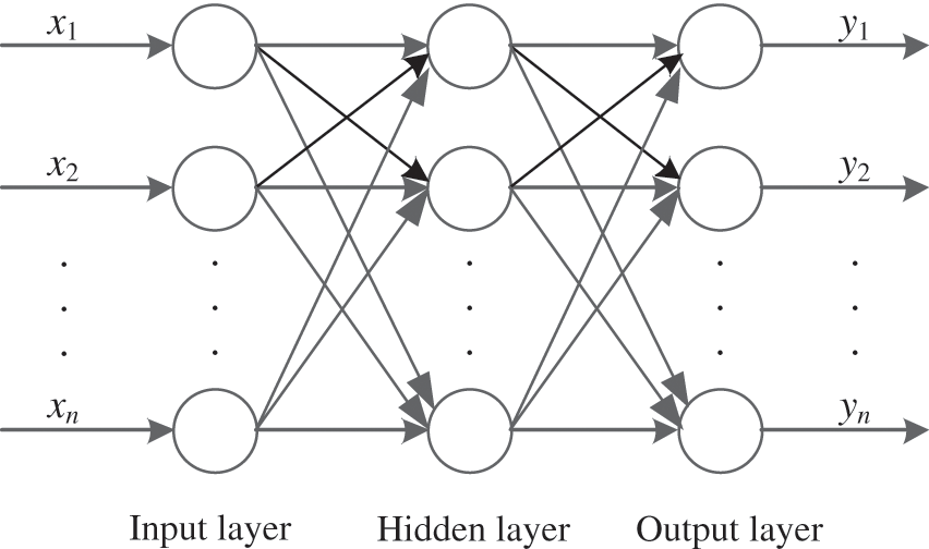
Figure 3: Topology of a BP network

The central idea of a BP network is that the sum of squared errors in the last layer is used as the cost function. To obtain the optimal cost function value, we need to modify the weights and thresholds of the network iteratively. The process is adjusted using the gradient descent method. The training and optimization of the whole process are achieved when the modified optimized value is less than or equal to the set error value. The algorithm flow of a BP network can be illustrated in Fig. 4.

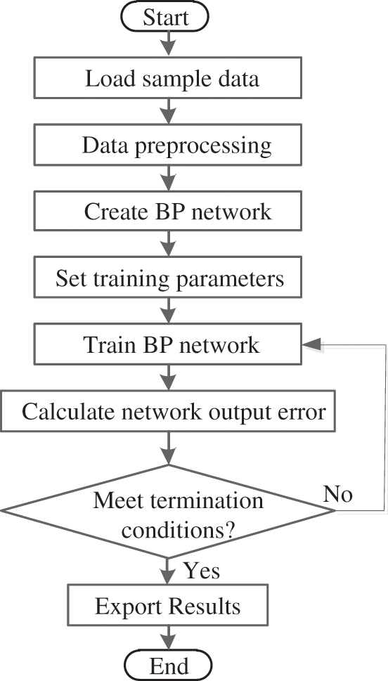
Figure 4: Algorithm flow in a BP network

3.2 Fault Diagnosis with the ASAPSO Algorithm

3.2.1 PSO Algorithm

Dr. Eberhart and Dr. Kennedy proposed the particle swarm optimization (PSO) algorithm in 1995. It is based on the concepts of population and evolution. It searches for an optimum solution in a D-dimensional target space [28,29]. If the population size is N, then the position of the ith particle is

Xi=(xi1,xi2,…,xiD),i=1,2,…,N(1)

The velocity of the ith particle is

Vi=(vi1,vi2,…,viD),i=1,2,…,N(2)

As the ith particle evolves from generation t to generation t + 1, its position and velocity are updated:

vt+1iD=ωvtiD+c1r1(ptiD−xtiD)+c2r2(ptgD−xtiD)(3)

xt+1iD=xtiD+vt+1iD(4)

where ω is the inertia coefficient, c1 is the self-cognitive factor, c2 is the socio-cognitive factor, r1, and r2 are random numbers distributed in the range [0, 1], PtiD is the extreme individual value, and PtgD is the extreme global value.

When searching for the optimum, the particle is mainly guided by its previous velocity and two learning factors. ω is the inertia part that guides how the particle retains its original velocity. c1 is the self-cognitive part, which guides the particle flying to its historical best position. c2 is the socio-cognitive component, guiding the particles to the best place in the population or neighborhood history. Commonly, the iterative search in the PSO algorithm terminates when the fitness is sufficiently accurate, or the set number of evolutions is reached. In this paper, to fully evaluate and analyze the effects of various algorithms, the process stops after a set number of iterations.

After the two core parameters of the particle, the velocity and position, are updated, the boundary is checked to determine whether the range has been exceeded. If it has, the current value is replaced with a random value within the field or directly with the boundary value. The article is updated using the individual and global extremes:

pt+1iD={xtiD,f(xtiD)≤f(ptiD)ptiD,f(xtiD)>f(ptiD)(5)

pt+1gD={ptiD,f(ptiD)≤f(ptgD)ptgD,f(ptiD)>f(ptgD)(6)

Because BP networks have a slow convergence rate and are prone to converge to a local optimum, the PSO algorithm is adopted in this study to obtain the optimum values of the initial parameters of the network. The basic idea is that the BP network’s neuron connection rights and thresholds are regarded as one particle. The high-dimensional parameter space, composed of the weights and thresholds, is searched to find an optimal solution. The PSO algorithm replaces the algorithm for backpropagating errors in the BP network. It finds all the initial optimal parameter values for the network when the objective function is minimized. The flow in a BP network optimized with the PSO algorithm is illustrated in Fig. 5.

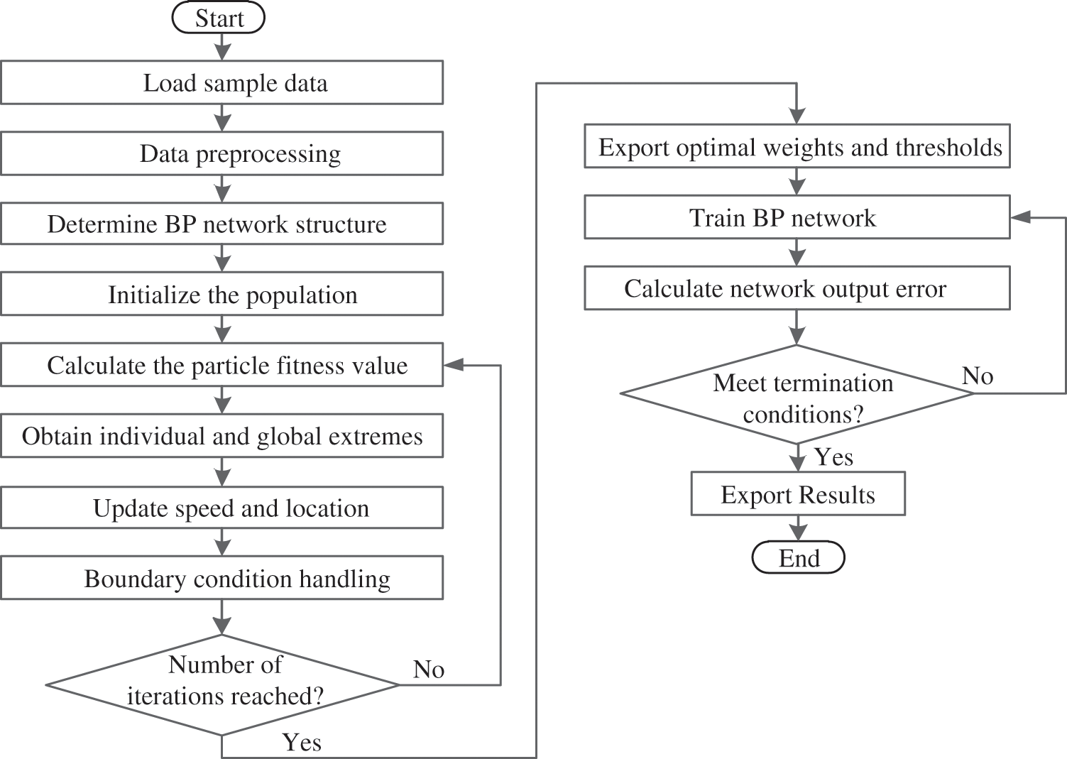
Figure 5: Algorithm flow in a BP network optimized with the PSO algorithm

3.2.2 Simulated Annealing

SA is employed for solving global optimization problems based on Monte Carlo ideas. It has been widely used as it is effective in solving combinatorial optimization problems and complex function optimization problems [30]. The Metropolis criterion is at the core of the SA algorithm. This method is unique in that it accepts better values of the objective function during the iterative process, and it can also obtain worse values with some probability [31]. The SA algorithm is incorporated into the PSO algorithm, as it can help particles jump out of a local optimum effectively. It also speeds up the calculation and enhances the quality of the solution.

The SA algorithm generates a new solution and determines whether it can be accepted in three main steps:

1.    The temperature and the solution are set initially.

2.    The probability of receiving a new solution during each iteration is derived from the current temperature.

3.    The temperature is updated based on whether it performs the annealing operation.

First, the initial temperature of the SA algorithm is set according to the global optimum value of the initial state of the particle swarm. The temperature in each outer loop iteration is updated according to a decay function. In this paper, we use an exponential decay function:

T(t)={E(ptgD)/log⁡(0.2),t=1αT(t−1),t>1(7)

where E(ptgD) represents the overall optimal value of the population at the initial stage, and α is a cooling constant, which is in the range of 0 to 1, but is generally very close to 1.

Second, after the initial temperature of the population is set at the early stage of the iteration, a new solution is accepted during each iteration according to the Metropolis sampling criterion. The acceptance probability is

pi(t)={1,Ei(t)<Egexp⁡(−Ei(t)−EgTi),Ei(t)≥Eg(8)

where Ei(t) represents the individual extremum of a single particle at the ith iteration, Eg represents the optimal extremum of the whole population, and Ti represents the current temperature. The temperature in each iteration decays linearly according to Eq. (7). If after an iteration Ei(t) < Eg, then this solution is adopted and used to replace the previous optimal solution. At the same time, it automatically updates the objective value. Otherwise, it will not fully accept the new solution, and the probability of acceptance isexp⁡(−ΔE/Ti) .

Third, if the termination condition of the algorithm is met, the program exits, and the current solution is chosen as the optimum. The annealing operation is then performed to update the temperature.

The whole optimization search process with the SA algorithm is an alternative process. It constantly searches for a new solution with a slow cooling down. A Markov process can describe this step. Each new state Ei(t + 1) is produced independently of the previous initial solutions from Ei(0) to Ei(t − 1), as it is entirely determined by Ei(t). It is asymptotically convergent and has a probability of 1 that it will connect to the global optimum. The most significant advantage of the SA algorithm is that because it searches probabilistically, particles do not get trapped in a local optimum, which improves the probability of finding the global optimum.

3.2.3 ASAPSO Algorithm

The velocity and accuracy of the PSO algorithm in the search process are mainly influenced by three control parameters: ω, c1, and c2. The inertia factor ω especially balances the overall capability of the algorithm. It is set to larger values in the early stages of the evolution. In the early evolutionary stage, c1 is set to a significant discount, gradually decreasing. In contrast, c2 has a small matter that gradually increases. The learning factors c1 and c2 mainly regulate the maximum flight lengths of particles toward the individual and global extremes, respectively. The direction of the flight of the particles is affected by these three parameters together, and the overall result is that better particles are found.

A negative hyperbolic tangent function is used to update the inertia weight adaptively:

ω=(ωmax+ωmin)2+tanh⁡(−4+8(kmax−k)kmax)(ωmax−ωmin)2(9)

where k represents the present number of evolutions, kmax represents the allowed maximum number of evolutions, while ωmin and ωmax represent the minimum and maximum of the inertia weights, respectively.

This function is a nonlinear control strategy. At the beginning of the algorithm, ω is large and decreases slowly so that the particles are given sufficient time to search globally. This ensures that the parameter space is searched globally. During the middle period, ω decreases approximately linearly, gradually increasing the particle’s local search capability. In the later search stage, the rate of change of ω is reduced again to ensure that the particles perform a careful local search near the extreme point, allowing the algorithm to obtain the global optimum accurately. Thus, the particles’ global and regional search abilities are balanced by dynamically adjusting ω.

In this study, after many experimental tests, the PSO algorithm achieved the best performance when ωmin = 0.4 and ωmax = 0.95. The inertia weight is plotted in Fig. 6.

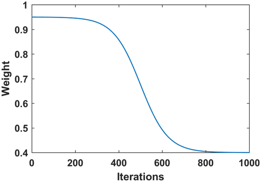
Figure 6: Adaptive change of the inertia weight

The two learning factors are adaptively updated linearly. At the beginning of the search, c1 is given a significant positive value, and c2 is provided a small positive value. As the investigation progresses, c1 is linearly and gradually decreased, and c2 is linearly and progressively increased so that the focus of the inquiry by a particle is adjusted at different stages. The expressions for c1 and c2 are

c1=c1max−k(c1max−c1min)kmax(10)

c2=c2min+k(c2max−c2min)kmax(11)

where c1min and c1max are the minimum and maximum of the individual learning factor, respectively, and c2min and c2max are the minimum and maximum of the population learning factor, respectively. In this study, we determined the reasonable values of these four parameters after several experimental tests. When c1min = c2min = 1.2 and c1max = c2max = 2.55, the convergence rate of the PSO algorithm was reasonable; in optimization with the PSO algorithm, the transfer of particles must be done clearly. However, this certainty may cause particles to fall into a local optimum. To increase the flexibility of the search process, we have used the SA algorithm in this paper to improve its convergence rate.

The SA algorithm can accept the optimal value when the temperature decreases and retain a different deal with a certain probability. The initial temperature of SA is set based on the optimal value of the initial state of the population at the beginning of each iteration. During iteration, the difference between the updated individual particle fitness and the current population optimal fitness is calculated with the Metropolis criterion. Then, the probability pi(t) of receiving the new solution is obtained according to Eq. (8). A comparison with rand() is used to decide whether to accept a worse value. Finally, the annealing operation is performed to update the temperature.

In summary, in the ASAPSO algorithm proposed in this paper, the three critical parameters of the PSO algorithm are updated adaptively. In addition, the SA operation is incorporated to increase the possibility of the algorithm performing a global search. Thus, the optimization rate and the accuracy of the algorithm’s convergence are improved. In combination with the sample of fault features obtained previously, the specific steps in the ASAPSO algorithm for optimizing the parameters of a BP network and using it to diagnose faults are as follows:

Step 1: Preprocess the feature information data set.

Step 2: Construct the BP network, and configure the network parameters.

Step 3: Set the parameters of the PSO algorithm, and initialize the population.

Step 4: Evaluate the fitness values of the initial particles. Record the extreme individual value PtiD and the extreme global value PtgD. Determine the initial temperature for SA with Eq. (7).

Step 5: Adaptively update the parameters ω, c1, and c2 according to Eqs. (9) to (11).

Step 6: Update the two parameters, velocity and position, according to Eqs. (3) and (4).

Step 7: Calculate the value of the objective function of the updated particles.

Step 8: Update the individual best position of the particle with Eq. (5) and the overall best position with Eq. (6).

Step 9: Calculate the probability pi(t) of accepting a new solution at the current temperature with Eq. (8).

Step 10: Compare pi(t) and rand() to determine whether the global optimum replaces the new solution, and then perform the cooling operation to update the temperature.

Step 11: Stop the search if the evolutionary number kmax is reached. Otherwise, return to step (5) to continue the search.

Step 12: Identify the current global optimal particles.

Step 13: Train the BP neural network.

Step 14: Calculate the network error.

Step 15: If the error accuracy requirement is not satisfied, return to step (13).

Step 16: Output the fault diagnosis classification, and terminate the algorithm.

4  Results and Discussion

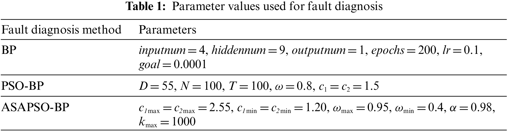
To assess the fault classification effectiveness of the ASAPSO algorithm, we compared it with two other methods. The relevant parameters are set in Table 1.

4.1 Fault Classification by a BP Network

Before training the BP network, we need to determine its overall structure. The more layers there are, the more the output error is reduced, so the network output will be closer to the expected value. However, as the number of layers in a network increases, the structure of a network becomes more complex, and the training time is also prolonged. Because an arbitrary nonlinear function can be approximated with a three-layer BP network, the number of layers was determined to three. The network is configured as follows. According to Section 2, we know that the information input about fault features has four components, so the first layer was set to four nodes. The coding bits for classifying the fault output consist of one decimal number, so the output layer was assigned to one node. Unlike before, there is no fixed rule for the hidden layer. Thus, a reasonable value needs to be selected through trial and error. After repeated training and analysis of the experimental results, the hidden layer was finally determined to be nine nodes; thus, the overall structure was determined to be 4-9-1.

The sigmoid function was used for the hidden layer, while the linear function was used for the output layer. The network is trained using the L–M training function. The other parameters are listed in Table 1. All the fault information for the rectifier circuit at trigger angles α = 0°, 30°, 60°, and 90° was selected as training samples. The number of training samples was 88. Different sampling times were chosen for each trigger angle for sampling multiple faults. The information acquired about the mark was used to form 66 test samples. The simulation results of fault classification by the BP network are illustrated in Fig. 7. The horizontal coordinate represents the index of the test sample, and the vertical coordinate is the fault category. The accuracy rate of fault classification was 78.78%.

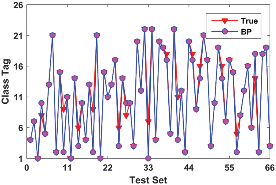
Figure 7: Fault classification with BP network

4.2 Optimization of Fault Classification of a BP Network by the PSO Algorithm

The PSO algorithm was used to globally optimize the parameters of the BP network in this paper. Initially, we need to define the number of weights and thresholds. The configuration of the BP network was the same as in Section 4.1, namely 4-9-1. Thus, it can be calculated that the number of codes required was 55. Table 1 lists the parameter values used in the PSO algorithm. Fig. 8 illustrates the simulation results of fault classification by PSO-BP. It can be seen that the accuracy rate of fault classification was 86.36%. This result shows that the BP network is optimized with the PSO algorithm, dramatically improving fault diagnosis accuracy.

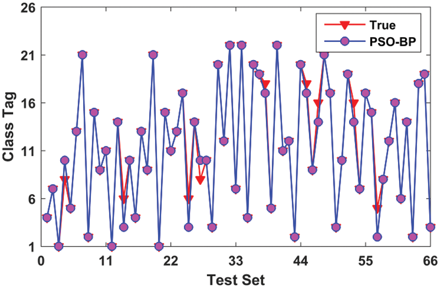
Figure 8: Fault classification with PSO-BP

4.3 Optimization of Fault Classification of a BP Network by the ASAPSO Algorithm

To improve diagnostic accuracy, we have used the SA algorithm in this paper to update the three critical parameters of the PSO algorithm adaptively. Table 1 lists the parameter values used in the ASAPSO algorithm. The other parameter values and the network structure were the same as before. Fig. 9 illustrates the simulation results of fault diagnosis by the ASAPSO-BP algorithm. It can be seen that the accuracy rate of fault classification reached 95.45%. In conclusion, the BP neural network optimized with the ASAPSO algorithm has higher fault diagnosis accuracy. Therefore, it is more suitable for diagnosing faults in power circuits.

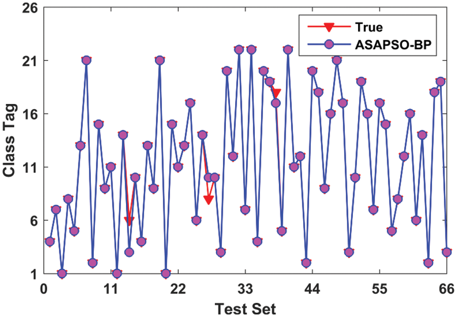
Figure 9: Fault classification with ASAPSO-BP

5  Conclusions

In this research, we propose an ASAPSO algorithm to optimize the internal parameters of a BP network and use it to diagnose faults in power electronic circuits. The components of the fault voltage signal were extracted by Fourier analysis, and sample data were obtained using the harmonic components. After normalization, the data were input as the training sample to optimize the BP network. We used a negative hyperbolic tangent function to adjust for nonlinear changes in the inertia weights ω and a linear change strategy to update the learning factors c1 and c2. Thus, the three crucial search parameters of the PSO algorithm were updated adaptively in each iteration. An SA operation was introduced into the iteration process to give the particles a higher chance of moving away from a local optimal. Overall, the searchability of the PSO algorithm was greatly improved, and the search requirements for the algorithm at different stages were met. It can be concluded from the experimental results that the optimization rate and fault diagnosis accuracy of the algorithm has been significantly improved. This diagnostic strategy could be extended to multiphase multilevel circuits.

Funding Statement: This work was supported by the 2022 Project for Improving the Basic Research Ability of Young and Middle-aged Teachers in Guangxi Universities (Grant No. 2022KY0209).

Conflicts of Interest: The authors declare that they have no conflicts of interest to report regarding the present study.

References

1. X. Pei, S. Nie, Y. Chen and Y. Kang, “Open-circuit fault diagnosis and fault-tolerant strategies for full-bridge DC–DC converters,” IEEE Transactions on Power Electronics, vol. 27, no. 5, pp. 2550–2565, 2012. [Google Scholar]

2. W. -C. Wang, L. Kou, Q. -D. Yuan, J. -N. Zhou, C. Liu et al., “An intelligent fault diagnosis method for open-circuit faults in power-electronics energy conversion system,” IEEE Access, vol. 8, pp. 221039–221050, 2020. [Google Scholar]

3. J. Wang, H. Ma and Z. Bai, “A submodule fault ride-through strategy for modular multilevel converters with nearest level modulation,” IEEE Transactions on Power Electronics, vol. 33, no. 2, pp. 1597–1608, 2018. [Google Scholar]

4. P. Kandasamy and K. Prem Kumar, “Efficient single-stage bridgeless ac to dc converter using grey wolf optimization,” Computer Systems Science and Engineering, vol. 43, no. 2, pp. 487–499, 2022. [Google Scholar]

5. X. Ge, J. Pu, B. Gou and Y. -C. Liu, “An open-circuit fault diagnosis approach for single-phase three-level neutral-point-clamped converters,” IEEE Transactions on Power Electronics, vol. 33, no. 3, pp. 2559–2570, 2018. [Google Scholar]

6. Z. Gao, C. Cecati and S. X. Ding, “A survey of fault diagnosis and fault-tolerant techniques—Part I: Fault diagnosis with model-based and signal-based approaches,” IEEE Transactions on Industrial Electronics, vol. 62, no. 6, pp. 3757–3767, 2015. [Google Scholar]

7. D. Zhang, L. Qian, B. Mao, C. Huang, B. Huang et al., “A data-driven design for fault detection of wind turbines using random forests and XGboost,” IEEE Access, vol. 6, pp. 21020–21031, 2018. [Google Scholar]

8. Z. Li, Y. Gao, X. Zhang, B. Wang and H. Ma, “A model-data-hybrid-driven diagnosis method for open-switch faults in power converters,” IEEE Transactions on Power Electronics, vol. 36, no. 5, pp. 4965–4970, 2021. [Google Scholar]

9. Y. Chen, Z. Li, S. Zhao, X. Wei and Y. Kang, “Design and implementation of a modular multilevel converter with hierarchical redundancy ability for electric ship MVDC system,” IEEE Journal of Emerging and Selected Topics in Power Electronics, vol. 5, no. 1, pp. 189–202, 2017. [Google Scholar]

10. M. D. Shieh and C. C. Yang, “Classification model for product form design using fuzzy support vector machines,” Computers & Industrial Engineering, vol. 55, no. 1, pp. 150–164, 2008. [Google Scholar]

11. M. Aly, E. M. Ahmed and M. Shoyama, “A new single-phase five-level inverter topology for single and multiple switches fault tolerance,” IEEE Transactions on Power Electronics, vol. 33, no. 11, pp. 9198–9208, 2018. [Google Scholar]

12. J. Poon, P. Jain, I. C. Konstantakopoulos, C. Spanos, S. K. Panda et al., “Model-based fault detection and identification for switching power converters,” IEEE Transactions on Power Electronics, vol. 32, no. 2, pp. 1419–1430, 2017. [Google Scholar]

13. W. Gong, H. Chen, Z. Zhang, M. Zhang and H. Gao, “A data-driven-based fault diagnosis approach for electrical power DC-DC inverter by using modified convolutional neural network with global average pooling and 2-D feature image,” IEEE Access, vol. 8, pp. 73677–73697, 2020. [Google Scholar]

14. A. Moradzadeh, B. Mohammadi-Ivatloo, K. Pourhossein and A. Anvari-Moghaddam, “Data mining applications to fault diagnosis in power electronic systems: A systematic review,” IEEE Transactions on Power Electronics, vol. 37, no. 5, pp. 6026–6050, 2022. [Google Scholar]

15. B. Cai, Y. Zhao, H. Liu and M. Xie, “A data-driven fault diagnosis methodology in three-phase inverters for PMSM drive systems,” IEEE Transactions on Power Electronics, vol. 32, no. 7, pp. 5590–5600, 2017. [Google Scholar]

16. R. Wang, Y. Zhan, H. Zhou and B. Cui, “A fault diagnosis method for three-phase rectifiers,” International Journal of Electrical Power and Energy Systems, vol. 52, no. 1, pp. 266–269, 2013. [Google Scholar]

17. K. Sarita, S. Kumar and R. K. Saket, “OC fault diagnosis of multilevel inverter using SVM technique and detection algorithm,” Computers & Electrical Engineering, vol. 96, pp. 107481, 2021. [Google Scholar]

18. V. Gomaty and S. Selvaperumal, “Fault detection and classification with optimization techniques for a three-phase single-inverter circuit,” Journal of Power Electronics, vol. 16, no. 3, pp. 1097–1109, 2016. [Google Scholar]

19. Y. Xue, T. Tang and A. X. Liu, “Large-scale feedforward neural network optimization by a self-adaptive strategy and parameter based particle swarm optimization,” IEEE Access, vol. 7, pp. 52473–52483, 2019. [Google Scholar]

20. F. Han, W. -T. Chen, Q. -H. Ling and H. Han, “Multi-objective particle swarm optimization with adaptive strategies for feature selection,” Swarm and Evolutionary Computation, vol. 62, pp. 100847, 2021. [Google Scholar]

21. J. -J. Jiang, W. -X. Wei, W. -L. Shao, Y. -F. Liang and Y. -Y. Qu, “Research on large-scale bi-level particle swarm optimization algorithm,” IEEE Access, vol. 9, pp. 56364–56375, 2021. [Google Scholar]

22. C. Chen and C. Li, “Process synthesis and design problems based on a global particle swarm optimization algorithm,” IEEE Access, vol. 9, pp. 7723–7731, 2021. [Google Scholar]

23. P. Dziwiński and Ł. Bartczuk, “A new hybrid particle swarm optimization and genetic algorithm method controlled by fuzzy logic,” IEEE Transactions on Fuzzy Systems, vol. 28, no. 6, pp. 1140–1154, 2020. [Google Scholar]

24. A. Shoukat, M. Ali Mughal, S. Younus Gondal, F. Umer, T. Ejaz et al., “Optimal parameter estimation of transmission line using chaotic initialized time-varying pso algorithm,” Computers, Materials & Continua, vol. 71, no. 1, pp. 269–285, 2022. [Google Scholar]

25. A. Sai Sarathi Vasan, B. Long and M. Pecht, “Diagnostics and prognostics method for analog electronic circuits,” IEEE Transactions on Industrial Electronics, vol. 60, no. 11, pp. 5277–5291, 2013. [Google Scholar]

26. J. Liu, J. Huang, R. Sun, H. Yu and R. Xiao, “Data fusion for multi-source sensors using GA-PSO-BP neural network,” IEEE Transactions on Intelligent Transportation Systems, vol. 22, no. 10, pp. 6583–6598, 2021. [Google Scholar]

27. Z. Dong, C. Wu, X. Fu and F. Wang, “Research and application of back propagation neural network-based linear constrained optimization method,” IEEE Access, vol. 9, pp. 126579–126594, 2021. [Google Scholar]

28. U. Geetha and S. Sankar, “Multi-objective modified particle swarm optimization for test suite reduction (mompso),” Computer Systems Science and Engineering, vol. 42, no. 3, pp. 899–917, 2022. [Google Scholar]

29. C. W. Hung, W. L. Mao and H. Y. Huang, “Modified pso algorithm on recurrent fuzzy neural network for system identification,” Intelligent Automation & Soft Computing, vol. 25, no. 2, pp. 329–341, 2019. [Google Scholar]

30. T. Wang, P. Shao, S. Liu, G. Li and F. Yang, “A multi-mechanism particle swarm optimization algorithm combining hunger games search and simulated annealing,” IEEE Access, vol. 10, pp. 116697–116708, 2022. [Google Scholar]

31. Y. Zhou, W. Xu, Z. -H. Fu and M. Zhou, “Multi-neighborhood simulated annealing-based iterated local search for colored traveling salesman problems,” IEEE Transactions on Intelligent Transportation Systems, vol. 23, no. 9, pp. 16072–16082, 2022. [Google Scholar]