An Effective Runge-Kutta Optimizer Based on Adaptive Population Size and Search Step Size

1  Introduction

Many real-world problems in diverse fields such as engineering [1], machine learning [2], finance [3], and medicine [4] can be formulated as optimization problems. Metaheuristic algorithms have become the most widely used technique for quickly discovering effective solutions to challenging optimization problems due to their adaptability and simplicity of implementation. However, to enhance the performance of these algorithms, various parameters must always be tuned. In general, metaheuristic algorithms are designed based on four types of processes, such as swarm, natural, human, and physics [5]. Particle Swarm Optimization (PSO) [6] is a widely used technique that depends on the natural behavior of swarming particles. Genetic Algorithm (GA) [7], which is the most often used evolutionary approach, is an efficient algorithm for a variety of real-world problems. The socio-evolution learning optimizer [8] is constructed by simulating human social learning in social groups such as families. The multi-verse optimizer [9] is based on the multi-verse theory proposed by physics and has addressed several problems, including global optimization, feature selection, and power systems. The sine cosine algorithm (SCA) [10] is another physics-based optimizer [5].

The search strategy, the exploitation phase, and the exploration phase are three key features shared by all metaheuristic algorithms. In the exploration phase, the metaheuristic algorithm generates random variables to search the complete solution space and examines the promising region, but in the exploitation phase, the algorithm searches close to the optimal solutions to obtain the best outcome from the search space. To prevent reaching the local optimum and keep enhancing the solution’s quality, the optimization algorithm must balance the exploitation and exploration stages [11]. In addition, running such algorithms can lead to environmental issues such as carbon footprints. The carbon footprint typically calculates the amount of greenhouse gas (GHG) produced during the execution of the algorithm. As a result, to develop green computing, it is critical to reduce unnecessary CO2 emissions and calculate the carbon footprint of the running algorithm because the carbon footprint relies on the energy used to power the device. Green computing will be shaped by understanding the behavior of the algorithm, avoiding unused runs, and minimizing factors that have a significant influence on the carbon footprint [12].

To solve a wide range of optimization problems, the RUN [13] population-based optimization algorithm was developed. As a search mechanism, RUN uses the principle of slope variations calculated using the Runge Kutta (RK) approach [13,14]. RK is a numerical method for integrating ordinary differential equations by using multistage approaches in the middle of an interval to generate a more accurate solution with a lower amount of error. This search approach makes use of two effective exploitation and exploration stages to find attractive areas in the search space and progress to the optimal global solution [13]. Despite RUN being a recent algorithm, it has demonstrated excellent performance in solving complex real-world problems such as parameters estimation of photovoltaic models [15,16], power systems [17,18], lithium-ion batteries management [19], identification of the optimal operating parameters for the carbon dioxide capture process in industrial settings [20], water reservoir optimization problems [21], resource allocation in cloud computing [22], and machine learning models parameters tuning [23] to name a few.

However, it was noticed that the original RUN consumes more time in solving optimization problems without finding the optimal solution, and in high-dimensional problems, the search capabilities and convergence speed of the original RUN deteriorate. As a result, to locate the optimal solution, the max number of iterations should be increased, so RUN’s runtime will increase. To overcome these issues, this work proposes an improved version of the original RUN called the Adaptive-RUN algorithm intending to obtain a specific level of precision in the solution with the least amount of computing cost, effort, and time, and to aid in the development of green computing. Population size adaption has become prevalent in many population-based metaheuristic algorithms to enhance their efficiency [5]. However, none of the reported works have considered population size adaptation to enhance the performance of RUN. To fill this research gap, unlike the original RUN where population size is fixed in every iteration, Adaptive-RUN will adaptively change population size to enhance runtime characteristics of both the exploitation and exploration phases of the algorithm. Furthermore, the proposed technique employs the adaptive search step size to determine and update the better solution in the early stages of evaluation, so the solution quality will be enhanced, and the algorithm will find the best solution quickly by minimizing the objective function toward an optimal solution. Therefore, the key contributions of this study can be summarized as the following:

– Propose an Adaptive-RUN algorithm that automatically adjusts population size during the search process according to two population size adaptation techniques, which are linear staircase reduction and iterative halving, by effectively balancing exploitation and exploration characteristics of the original RUN algorithm. In addition, an adaptive search step size technique is employed to improve the solution quality, fitness, and convergence speed of the original RUN.

– Adaptive-RUN performance is analyzed over 23 IEEE CEC-2017 benchmark functions for two cases, where the first one applies linear staircase reduction with adaptive search step size (LSRUN), and the second one applies iterative halving with adaptive search step size (HRUN), with the original RUN and three recent metaheuristic algorithms. To promote green computing, the carbon footprint metric is included in the performance evaluation.

– Simulation results based on the Friedman and Wilcoxon tests revealed that Adaptive-RUN can achieve considerable reductions in the average fitness, runtime, and carbon footprint values as compared to original RUN and other recent metaheuristic algorithms.

The rest of the paper is organized as follows: Section 2 provides an overview of related works. The main mathematical equations for RUN and the implementation of Adaptive-RUN are presented in Section 3. Section 4 examines the performance of Adaptive-RUN in tackling benchmark problems. Section 5 provides conclusions and some ideas for future studies.

2  Literature Review

In the solution space, optimization is utilized to determine the optimal solution. There exists a plethora of metaheuristics to solve optimization problems. All optimization strategies may be characterized as tackling the following optimization problem: minimize f(x), subject to g(x) <= 0, and h(x) = 0, where x is the set of values that need to be optimized, g(x) is a set of inequality constraints, and h(x) is a set of equality constraints. The objective of the optimization algorithm is to identify the values of x that minimize f(x) under the restrictions of g(x) = 0 and h(x) = 0 [24]. Ahmadianfar et al. [13] proposed the Runge Kutta optimizer (RUN). Based on the concept of the swarm-based optimization algorithm, RUN constructs a set of guidelines for population development and utilizes the estimated slope as a search method to identify the search space’s most likely region. The fourth-order Runge–Kutta (RK4) method is used to compute the slope and tackle ordinary differential equations. The RK4 depends on the weighted average of four slopes (k1,k2,k3,k4), and it can be described as y(x+Δx)=y(x)+16(k1+2k2+2k3+k4)×Δx, where y(x+Δx) is the approximate solution to a differential equation. k1 is the slope at the start of the time step, k2 and k3 are the slopes at the midpoint, and k4 is the slope at the endpoint. RUN begins the procedure with a selection of random solutions. For a population of size N, N positions are generated randomly in the first phase, and each individual in the population xn(1…N) is a solution. To add, the population is a set of solutions. The RK approach changes the positions of the solutions every time. The RK approach produces both a search mechanism and a solution. To choose between the exploitation (local) and exploration (global) stages, RUN uses the rand <0.5 rule, where a rand is a random value in [0,1]. RUN employs a local search to develop convergence speed and concentrate on superior solutions, while a global search is used to explore potential areas in space.

Additionally, to enhance the convergence rate and prevent local optimum solutions, the enhanced solution quality (ESQ) technique is utilized. ESQ guarantees that every individual advances to a better location and improves the quality of the solution. Two randomized variables are used by the search mechanism and ESQ to highlight the relevance of the optimal solution and move to the optimal global solution, which may successfully balance the exploitation and exploration phases. If the generated solution is not in a superior location to the present one, the RUN optimizer can find a new location in the search space to achieve a superior location. This process could potentially improve both the quality and rate of convergence. When RUN was compared to other modern optimizers, it was discovered that RUN outperformed other optimization algorithms in tackling complex real-world optimization problems [13].

In high-dimensional and difficult optimization problems, the RUN optimizer can struggle to avoid trapping in local minima. As a result, Devi et al. [11] proposed the improved Runge Kutta optimizer (IRKO), which is a better version of the RUN optimization algorithm. To improve the exploitation and exploration abilities, IRKO utilizes the local escaping operator (LEO) and the basics of RUN. LEO is used to improve the efficiency of a gradient-based optimizer, and it ensures the solution’s quality while improving convergence by preventing local minimum traps. The IRKO algorithm’s initialization process is equivalent to the RUN optimizer. In the search process, the RUN optimizer updated the population in three diverse stages. However, in the IRKO optimizer, the solutions are also examined during every iteration to investigate the offered solutions and enhance the new recommended solutions in the upcoming iteration. When every new population is generated at random, each population is evaluated, allowing the new fitness to be improved using either global or local search. The LEO process will then be used to enhance the new population. The results of IRKO were either better than or comparable to other algorithms, but IRKO’s runtime values are greater than the original RUN [11].

The RUN algorithm yields promising results, but it has limitations, especially when dealing with high-dimensional multimodal problems. As a consequence, Cengiz et al. [25] proposed the Fitness-Distance Balance (FDB) approach, which is used to produce solution candidates that control the RUN algorithm’s search operation. According to the reported experimental results, ten cases of FDB based on the RUN optimizer were created, tested, and verified one by one using experimental studies to locate the optimal solution in the RUN optimizer. The results show that the FDB-RUN approach [25] significantly improves the search process life cycle in the RUN optimizer and is considered more effective in solving high-dimensional problems by properly balancing the exploration and exploitation stages [25].

The population size plays a key role in both runtime efficiency and optimization effectiveness of metaheuristic algorithms [5]. Population size adaptation techniques automatically adjust population size during the search process and decide which members of the current population will proceed to the next iteration to achieve a good balance between exploration and exploitation characteristics. Although, population size adaptation has been widely studied in particle swarm intelligence [26], artificial bee colony optimization [27], differential evolution [28,29], sine cosine algorithm [5], and slime mould algorithm [30] among others. However, to the best of the author’s knowledge, no such work has been reported for the RUN. This work aims at filling this gap by examining two different population size adaptation methods applied previously [5] in the proposed Adaptive-RUN algorithm. In addition, we employed the concept of adaptive step size from the seeker optimization algorithm (SOA) proposed by Dai et al. [31]. The adaptive step size in the proposed study is a kind of a look-ahead technique to determine a search direction and search step size for each individual whenever the population size changes for fast convergence of the algorithm.

3  Methodology

3.1 Runge Kutta Optimizer (RUN)

The RUN depends on mathematical structures and lacks metaphors. The RUN optimizer utilizes the Runge Kutta method (RK) [14] as a search mechanism to productively accomplish the search process by balancing the exploitation and exploration phases. To tackle ordinary differential equations (ODEs) by applying a distinctive formula, the RK method is utilized. Also, the enhanced solution quality (ESQ) structure is utilized in RUN to enhance the solutions’ quality and the convergence rate and avoid local optimum. In addition, each region in the solution space is supplied with random solutions. Then, a balance between the exploitation and exploration phases is accomplished by inserting a set of search solutions into the different regions. Moreover, the population is updated in three different phases in the life cycle of the RUN optimizer. As a result, the population xi is improved as xnew , xnew2, and xnew3 [13]. Only the major mathematical formulation for RUN will be addressed in the following subsections.

3.1.1 Search Mechanism

In RUN, the RK4 approach was used to define the search strategy, which depends on the weighted average of the four slopes as shown in Fig. 1. Eq. (1) represents the search mechanism (SM) in RUN.

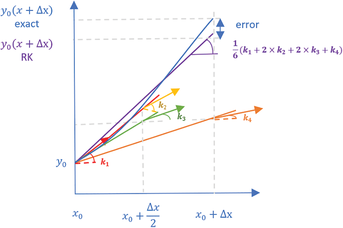
Figure 1: Slopes in the RK4 method

SM=16(xRK)×Δx(1)

xRK=k1+2×k2+2×k3+k4(2)

3.1.2 Updating Solutions

The RK4 method SM is utilized to develop the solutions in order to provide exploration and exploitation searches.

if rand<0.5(3)

 Exploration

xnew=(xC+g×r×xC×SF)+SM×SF+randn×μ×(xm−xC)

else

 Exploitation

xnew=(xm+g×r×xm×SF)+SM×SF+randn×μ×(xr1−xr2)

end

Note: xC and xm are defined in Eq. (4). SF stands for adaptable factor and is defined in Eq. (5). μ represents a random value in [0, 1]. randn produces a random scalar. r is a random value in [1, −1]. g is a random value in [0, 2]. xr1 and xr2 are two random solutions.

xC=xi×ϕ+xr1×(1−ϕ)(4)

xm=xbest ×ϕ+xlbest ×(1−ϕ)

Note: ϕ is a random value in [0, 1]. xi represents the individuals. xbest  is the optimal solution. xlbest  is the optimal current solution.

SF =2×f×(0.5− rand)(5)

f=exp⁡(−b×(ITMaxIT)×rand)×a(6)

Note: SF is an adaptive factor to provide a suitable balance between exploration and exploitation. f is a real number computed by using Eq. (6). The numbers a and b are constants, where a is initialized to 20 and b to 12. IT is the present iteration. The max number of iterations is known as MaxIT.

3.1.3 Enhanced Solution Quality (ESQ)

In order to optimize solution quality over the iterations while preventing local optimum, the RUN algorithm utilizes ESQ. The ESQ is used to produce the solution (xnew2).

xavg=xr3+xr2+xr13(7)

xnew1=xavg×β+xbest×(1−β)(8)

w=exp(−c(ITMaxIT))×rand(0,2)(9)

if rand<0.5(10)

  if w<1

xnew2=xnew1+w×r×|randn+(xnew1−xavg)|

 else

xnew2=(xnew1−xavg)+w×r×|randn+(xnew1×u−xavg)|

 end

end

Note: r is an integer value equal to −1, 0, or 1. c is a random value equal to 5 × rand. β is a random value in [0, 1]. xr1, xr2, xr3 are three random solutions.

if rand<w(11)

xnew3=(xnew2−xnew2×rand)+((xb×v−xnew2)+SM)×SF

end

Note: v is a random value that equals 2 × rand. xb is the best solution.

3.1.4 Optimization Process in RUN

Fig. 2 shows that RUN starts with the RK search mechanism to update the solution position, then employs ESQ to explore the promising regions in the search space. Then the selection of the best solution will be done. The position xnew will be generated from position xi using the RK method, and xnew2 will be generated using ESQ. If fitness of xnew2 is less than fitness of xnew, xnew2 is the best solution; otherwise, xnew3 position will be generated, and if fitness of xnew3 is less than fitness of xnew, xnew3 is the best solution; otherwise, xnewis the best solution.

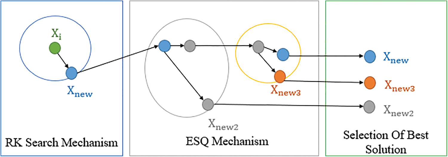
Figure 2: Optimization process in RUN

3.2 Adaptive-RUN

The RUN algorithm depends on the outcomes of the preceding iteration to generate new solutions. This can increase the runtime of the algorithm and slow its convergence speed. In this work, RUN is enhanced to balance the exploitation and exploration capabilities and improve the search capability using adaptive population size (PS) and adaptive search step size. The adaptive PS strategy will be applied before updating the solution (Eq. (3)). The adaptive PS strategy can decrease the runtime, increase the convergence speed, and improve fitness by moving members from the present population to the upcoming iteration, and the value of the population size will be changed. If the population size doesn’t equal the initial population size, the adaptive search step size strategy will be applied after updating the solution (Eq. (3)). The adaptive search step size strategy focuses on determining and developing a better alternative solution to quickly find the best solution by discovering the search step size and search direction and then updating the positions of the next individuals. The Adaptive-RUN optimizer provides a high convergence speed, a short runtime, and better fitness. In addition, two adaptive population strategies will be studied, where the first one will apply linear staircase reduction with adaptive search step size (LSRUN), and the second one will apply iterative halving with adaptive search step size (HRUN). This section will address the adaptive population size strategies (linear staircase reduction and iterative halving), and the adaptive search step size strategy.

3.2.1 Population Size Adaptation

The population size (PS) is a critical aspect that impacts how easy it is to locate the best solution in the search space. As a result, in metaheuristic algorithms, controlling the population size is considered important [5]. PS is a variable controlled by a user, and no research has investigated the impact of population size adaptation on RUN efficiency. So, the adaptive technique in which population size will change among iterations according to the requirements of the search process will be considered in this study. Two distinct adaptation techniques, linear staircase reduction RUN (LSRUN) and iterative halving RUN (HRUN), were chosen for study. The mathematical formulation will be addressed for linear staircase reduction and iterative halving in this section.

a) Linear Staircase Reduction

The linear staircase reduction decreases the runtime by moving random candidates to the next iteration [5,32]. Fig. 3a shows how the population size decreased over the iterations. If the current iteration (IT) happens to equal the reduction step (ITR), the population size (nP) will be reduced by the step factor (Step) using Eq. (12.2).

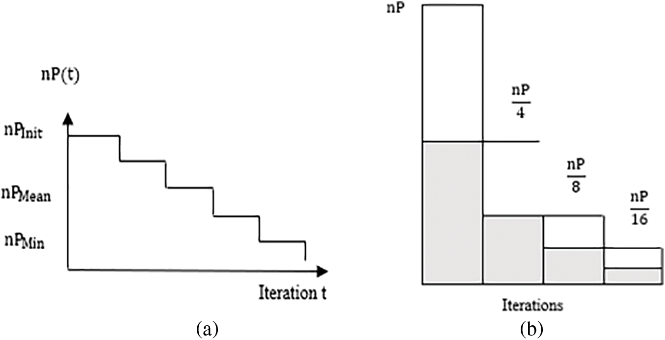
Figure 3: (a) Linear staircase reduction, (b) Iterative halving

NOR=(MaxPS−MinPS)/Step(12)

ITR=MaxIT/(NOR+1)(12.1)

if ITR==IT

nP=nP/Step(12.2)

end

Note: MaxPS is the max population size equal to 100 × nP. MinPS is the min population size equal to 100. NOR is the number of reductions. Step is the scaling factor equal to 2. ITR is the iteration when the reduction appears. nP is the population size and is initially set to 100.

b) Iterative Halving

Iterative halving moves the best candidates to the next iteration [5,33]. If the population size reaches the minimal population size (MinPS), the number of reductions (NOR) will be evaluated using Eq. (13.1); otherwise, Eq. (13.2). The fitness of the members from the first half of the present population will be compared to the fitness of the corresponding members from the second half using Eq. (13.5). Fig. 3b shows how iterative halving impacts the population size over the iterations by reducing the population size to half. If the fitness of the members from the second half is less than the fitness of the members from the first half, and the current iteration (IT) equals the reduction step (ITR), the members of the current population will be equal to the members from the second half (Eq. (13.6)), and the population size (nP) is halved (Eq. (13.7)).

if nP== MinPS

NOR=(log(MaxPS)−log(MinPS))(13)

else

NOR=(MaxPS−MinPS)/Step(13.1)

end

ITR=MaxIT/(NOR+1)(13.2)

index=(nP/2)+i(13.3)

ITR=MaxIT/(NOR+1)(13.4)

ifFobj(xindex)<Fobj(xi)andIT==ITR(13.5)

xi=xindex(13.6)

nP=(nP+1)/2(13.7)

end

3.2.2 Adaptive Search Step Size

If the optimal solution is not discovered in the early phases of evaluation, it might be easy to get stuck in the local optimum. So, it is considered essential to identify the search direction and search step size to update the next individuals’ positions. As a result, the local search ability will be enhanced, and if the lookahead better solution is determined and developed in the early stages of evaluation, the algorithm can locate the optimal solution rapidly. The idea of the adaptive search step size strategy is obtained from the seeker optimization algorithm (SOA) [31]. The adaptive search step size process in Adaptive-RUN includes three steps, which are: discover the search step size, discover the search direction, and update the solution [34]. To add, those steps are adopted from SOA. At each iteration in SOA, a search step size α and search direction d are independently evaluated for each individual. The search step size and search direction are defined by the SOA by mimicking the ambiguous reasoning of human search and the experience gradient. In RUN, we will use similar concepts to define the search step size and search direction.

Discover the Search Step Size: In the LSRUN and HRUN algorithms, after updating the solution xnew  using the Runge Kutta (RK) method (Eq. (3)), if the size of the population (nP) is reduced to half, the search step size α will be determined for the individuals to update the location of the solution xnew . α is the search step size, which is an array of real numbers of size set to the dimension size (α> 0). The parameters u, w, xmin, and xmax are utilized to express the search step size. Fitness includes the costs of each set of individuals sorted in descending order, the index includes the locations of the sorted costs, index(i) is the location of the cost at location i which is the location of the current individuals, u is a set of uniformly distributed random values in [0, 1], Umax is a constant value set to 0.9, Umin is a constant value set to 0.0111, w is a real number, w2max is a constant value set to 0.7, w2min is a constant value set to 0.2, xmin is the individuals with minimum cost, and xmax is the individuals with maximum cost. The optimal position of the individuals has Umax = 0.9, but the worst position has Umin = 0.0111. Umax is selected to be 0.9 to have a higher convergence rate and let the best individuals have an uncertain step size. The u function is selected as the fuzzy variable for the search step size α. The convergence behavior of the Adaptive-RUN is controlled by the deciding factor w. Low w will lead to local trapping, whereas high w will delay the algorithm’s convergence. As a result, for better searching, the w is determined as shown in Eq. (14.3). Furthermore, if the evolution algebra increases, w is decreased from w2max to w2min.

[fitness,index]=sort(Costs)(14)

u=Umax−index(i)/nP×(Umax−Umin)(14.1)

u=u×rand(1,dim)(14.2)

w=w2max−i/nP×(w2max−w2min)(14.3)

α=w×|xmin−xmax|×−log(u)(14.4)

Discover the Search Direction: In the LSRUN and HRUN algorithms, after updating the solution xnew  using the Runge Kutta (RK) method (Eq. (3)), if the size of the population (nP) is reduced to half, the search direction d will be determined for the individuals to update the location of the solution xnew . The search direction is determined by applying the weighted geometric in the manners described below (Eq. (14.5) to Eq. (14.8)) after determining the self-interest dego, the altruistic direction dalt, and the direction of action dproof any individual. d is the search direction, which is an array of 1 and −1 numbers of size equal to dimension size. d = 1 means that the individuals go toward the positive side of the coordinate axis, and d = −1 means the individuals go toward the negative side. gbest  is the population x which includes the sets of individuals/solutions, and it will be updated while determining the best solution, zbest  is the optimal solution that is found so far, xi is the individuals at the current location i, xit1 is the individuals at the location i from the previous iteration which can be written also as xi(IT−1) where IT is the current iteration, sign is a sign function, and ϕ1 and ϕ2 are constant values in [0,1].

dego=gbest−xi(14.5)

dalt=zbest−xi(14.6)

dpro=xit1−xi(14.7)

d=sign(w×dpro+ϕ1×dego+ϕ2×dalt)(14.8)

Update the Solution: After giving the search step α, search direction d, and search mechanism SM, the solution xnew  transfers to a new location from the current location (individuals) xi as shown in Eq. (14.9). SM is the search mechanism that is determined using Eq. (1).

xnew =xi+d×α×SM(14.9)

Fig. 4 shows how xnew  is updated on the search space based on the search step size, search direction, and SM values. Also, xi can update its position in different directions based on search step size, search direction, and SM. Search step size α and SM are arrays of real numbers, and they are used to search the feature space and design an appropriate global and local search; however, d is considered a direction controller as it is an array of 1 and −1. d also alters the search direction and expands diversity.

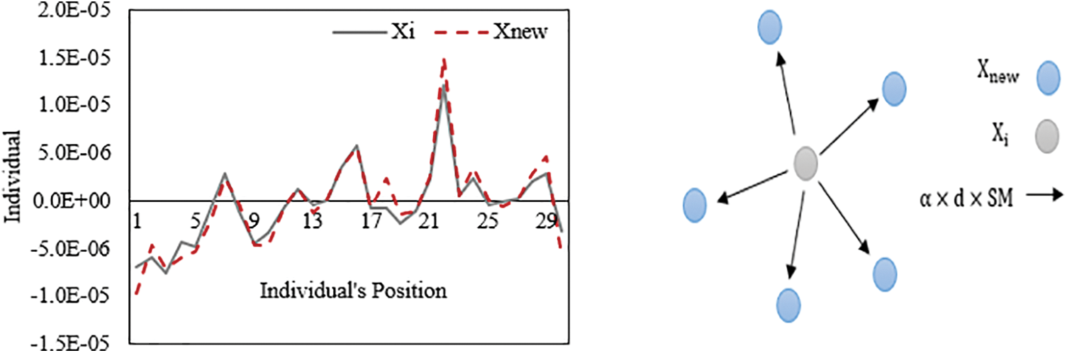
Figure 4: Solution update based on adaptive search step size mechanism

The Process of Adaptive Search Step Size: Fig. 5 shows the process of adaptive search step size in the Adaptive-RUN algorithm. Before applying the ESQ strategy, if the population size is changed, the process of adaptive search step size will start; otherwise, ESQ will start. The costs will be sorted, and xmin, xmax, gbest, zbest, SM, search step size, and search direction will be calculated before updating the solution xnew. Then the solution xnew  will be updated using Eq. (14.9). After that, the index i will be incremented (move to the second solution), and the cost of xnew  will be compared to the cost of xi (second solution). If the cost of xnew is less than the cost of xi,xi will be updated to xnew, and the cost of xi will be updated to the cost of xnew. As a result, the second solution will be determined and updated in the early stages of evaluation, and the algorithm will find the best solution quickly. In addition, the above values of the parameters Umin, Umax, w2max, w2min, ϕ1, and ϕ2 are selected after several trials of obtaining the best result. The best result means better fitness, convergence speed, and runtime.

Figure 5: Process of adaptive search step size

3.3 Pseudocode of Adaptive-RUN Algorithm

3.4 Complexity Analysis

The max number of iterations is called MaxIT, and the population size is called nP. nP is the number of solutions in the population. In RUN, the population size is fixed. However, in the Adaptive-RUN, the size of the population (nP) is dynamic. Initially, the size of nP in Adaptive-RUN is 100. After a number of iterations, nP will be 50. This means the number of computations and runtime will decrease. The Adaptive-RUN algorithm starts with population and cost initializations and a minimum fitness evaluation (xbest ). After that, the adaptive population strategy either linear staircase reduction or iterative halving will be applied. Then, minimum fitness, xw , xb  will be calculated followed by determining the new solution (xnew ) based on Runge Kutta (RK) method. Also, xnew  will be updated using the adaptive search step size strategy when the population size changes. In addition, the cost will be sorted during the adaptive search step size strategy. Then, xnew2  and xnew3  will be determined using an enhanced solution quality (ESQ). Finally, xbest  and gbest  will be updated. Let us assume nP is N. The computation cost (complexity) of population initialization (x) is O(N), cost initialization is O(N), minimum fitness evaluation (xbest ) is O(N), exploration of search space (evaluate xnew , xnew2  or xnew3 ) is O(1), parameter update (xb , xw , xbest , or gbest ) is O(1), and cost sorting is O(NlogN). Furthermore, the complexity of Adaptive-RUN cases (LSRUN and HRUN) is O(3N+MaxIT×N(7+N+NlogN)).

3.5 Flowchart of Adaptive-RUN

The flowchart of the Adaptive-RUN algorithm is shown in Fig. 6. The initialization process in Adaptive-RUN is similar to the original RUN. After calculating the fitness and the best solutions, one of the PS adaptive techniques (linear staircase reduction or iterative halving) will be applied. Then, xnew will be calculated via the search mechanism (SM) strategy. After that, if the population size is reduced to half, xnew will be updated via the adaptive search step size strategy. Finally, new solutions (xnew2 and xnew3) will be determined via an enhanced quality solution (EQS) strategy. So, the population is developed by search mechanism, adaptive search step size, and enhanced quality solution strategies. Adding the adaptive PS and adaptive search step size processes to RUN enhances the search capabilities, the quality of the solution, and the convergence rate of RUN.

Figure 6: Flowchart of adaptive-RUN

3.6 Key Features of Adaptive-RUN Compared to RUN

The search capabilities of RUN are decreased in high-dimensional problems. It is noticed that if the dimension size (search space size) of the problem in RUN is increased, the runtime of RUN will increase and the convergence speed will decrease, as shown in Fig. 7. Also, from Fig. 7, the value of the fitness increases which means the quality of the solutions is affected while increasing the dimensions. Most of the time, difficult real-world problems may have large dimension sizes, so the algorithm’s convergence rate will be slow, and to locate the best fitness, the max number of iterations may need to be increased. The Adaptive-RUN is used to improve the search capabilities (balance the exploitation and exploration phases), increase the convergence speed, and decrease the runtime by applying adaptive PS (linear staircase reduction or iterative halving) with an adaptive search step size. Adaptive PS decreases the runtime by moving random solutions to the next iteration, so the algorithm will focus on enhancing the quality of those solutions in the upcoming iterations. The adaptive search step size enhances the solutions’ quality, fitness value, convergence speed, and search capabilities by discovering the best solution in the early phases of evaluation. Fig. 8 shows that Adaptive-RUN runtimes outperform RUN runtimes with an increase in the number of iterations or dimension sizes.

Figure 7: In RUN, the relationship between dimension size and; (a) Runtime, (b) Fitness value

Figure 8: In RUN, the relationship between runtime and; (a) Dimension size, (b) Number of iterations

3.7 Optimization Process in Adaptive-RUN

Fig. 9 shows that the first process in Adaptive-RUN is population size adaptation, followed by the RK search mechanism. The population size adaptation method either linear staircase reduction or iterative halving will be applied to reduce the population size. Then a new solution xnew will be evaluated using RK. After that, if the population size is not equal to the initial population size, a new solution xnew will be evaluated using adaptive search step size then new solutions ( xnew2 and xnew3) will be evaluated using Enhanced Solution Quality (ESQ). Otherwise, if the population size is equal to the initial population size, we will not have the adaptive search step size process.

Figure 9: Optimization process in adaptive-RUN

4  Results and Discussion

The efficiency and performance of Adaptive-RUN cases (LSRUN and HRUN) are assessed using the IEEE CEC-2017 benchmark problems in a search space of dimension 30 [13,35]. The group of benchmark problems used in this study includes unimodal functions (F1–F7), basic multimodal functions (F8–F17), and fixed-dimension multimodal functions (F18–F23). The exploitative nature of various optimization algorithms can be tested using unimodal test functions (F1–F7). Multimodal functions (F8–F17) can test the optimization algorithms’ exploration and local optimum avoidance skills, and functions (F18–F23) show the capability of the algorithms to examine and explore the search spaces of low dimensions. The population size (nP) is set to 100, and the max number of iterations is set to 500. All results are reported after 20 independent runs. The experimental studies are implemented on MATLAB@ R2019b and 4 GB RAM and x64-based processor.

A comparison of the results of Adaptive-RUN cases with Slime Mould Algorithm (SMA) [36], Equilibrium Optimizer (EO) [37], Hunger Game Search (HGS) [38] and RUN [13] concerning performance metrics are reported in Table 1. As evident from Table 1 Adaptive-RUN cases have superior performance in all metrics as compared with RUN. Specifically, Adaptive-RUN cases obtain the best results in terms of runtime values for all the benchmark functions. This is due to the population size (PS) adaptation during the iterations using either the linear staircase reduction (LSRUN) or iterative halving (HRUN) strategy, and the adaptive search step size strategy, so the algorithm’s runtime and computation cost are reduced. In terms of average fitness, Adaptive-RUN exhibits better performance on 10 functions and equal performance on 13 benchmark functions (F2, F8, F9, F12, F13, F15, F17, F18, F19, F20, F21, F22, F23), which means Adaptive-RUN cases can produce high-quality solutions and better fitness values with lower runtime values than RUN. As compared with recent optimizers, Adaptive-RUN showed competitive performance.

To determine the average ranks of algorithms and show the differences between them, the Friedman test is applied to the average fitness and runtime values of all the optimizers. Table 2 shows the mean ranks of Adaptive-RUN and other algorithms for all the performance metrics on all the benchmark problems. From Table 2, LSRUN achieves the best rank in terms of all performance metrics, e.g., a mean rank of 2.76 in terms of average fitness values and a mean rank of 2.22 in terms of runtime. As a result, LSRUN has the best efficiency and performance as compared with the other algorithms. Furthermore, Table 2 shows the p-values of Friedman tests for all benchmark problems where considerable differences can be seen between Adaptive-RUN cases and other optimizers in terms of performance metrics values. Table 3 shows the Wilcoxon test for the runtime and average fitness values from the algorithms. From Table 3, it is noticed that Adaptive-RUN cases perform the best in terms of runtime and perform equal or better in terms of fitness (10 better and 13 equal) than the RUN optimizer, and there is no worse fitness in comparison with the RUN optimizer. To promote green optimization algorithms, the carbon footprint of the optimization algorithms [39] is computed. As a result, during the runtime of each algorithm, Microsoft Joulemeter [40] is used to measure the mean power consumption (P) of the MATLAB application. Then the application’s energy consumption is calculated for each algorithm using the equation E = Pt where t is the algorithm’s runtime. Depending on the emission factor for power consumption, for each algorithm, the carbon footprint is determined by transforming the application’s energy consumption (kWh) into CO2 emissions (0.25319 kgCO2ekWh). LSRUN achieved the best mean rank of 1.37 in terms of carbon footprint. We are not reporting the results of carbon footprints because of space limitations.

Convergence graphs are essential for assessing how well algorithms perform or which algorithms perform the best, and a good optimization algorithm is typically demonstrated by a smoothly decreasing convergence graph. Moreover, the convergence graph can be used to evaluate the performance of the optimization algorithm and can assist in determining if the algorithm has arrived at a good solution. As a result, the convergence graphs of Adaptive-RUN cases and RUN are displayed in Fig. 10 for some of the representative benchmark functions. Because of the appropriate balancing of the exploration and exploitation phases, the convergence graphs show that Adaptive-RUN cases, specifically LSRUN, have a faster convergence curve than RUN on unimodal and multimodal benchmark problems since the Adaptive-RUN cases can locate the optimal (best) solution in the early phases of evaluation. As a result, Adaptive-RUN cases provide a better and more proper convergence rate to improve and optimize the benchmark problems than RUN.

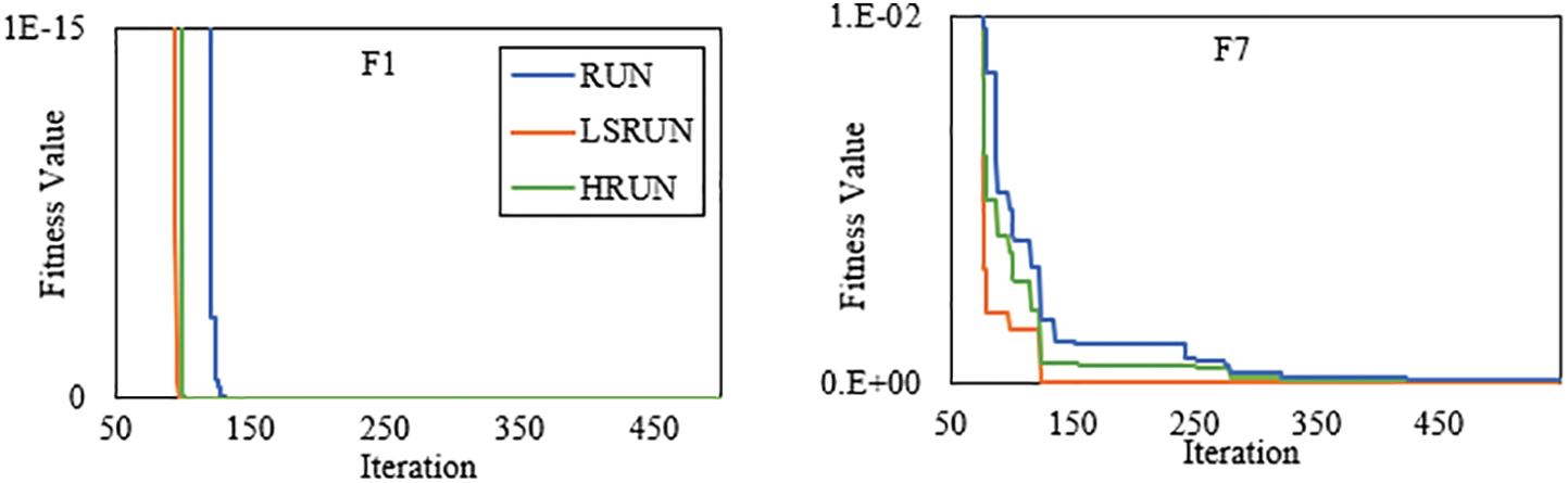
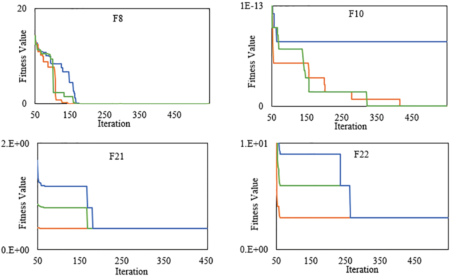
Figure 10: Convergence graph of adaptive-RUN (LSRUN and HRUN) and RUN

5  Conclusion

The Runge Kutta optimizer (RUN) is a recently developed population-based algorithm to solve a wide range of optimization problems [13]. However, in high-dimensional problems, the search capabilities, convergence speed, and runtime of RUN have deteriorated. To overcome these weaknesses, this study proposed the Adaptive-RUN algorithm, which employed adaptive population size and adaptive step size to enhance the performance of the RUN algorithm. Two cases of Adaptive-RUN were investigated where the first one applied linear staircase reduction in population with adaptive search step size (LSRUN), and the second one applied iterative halving in population with adaptive search step size (HRUN). The performance of the LSRUN and HRUN algorithms against the original RUN method was assessed using the unimodal, basic multimodal, and fixed-dimension multimodal test functions from the IEEE CEC-2017 benchmark problems. LSRUN and HRUN algorithms showed superior results in terms of solution quality, run time, and carbon footprint as compared to the original RUN algorithm as revealed by box plots, and the Wilcoxon and Friedman (ranking test) tests. Future work will investigate the impact of other population size adaptation approaches and parallelization of Adaptive-RUN in distributed computing platforms to further enhance its efficiency and scalability. In addition, the proposed work can be improved further by exploiting the problem-specific information based on the landscape of the search space.

Acknowledgement: The authors would like to thank Kuwait University for providing the computing resources to conduct this research. Thanks are also extended to anonymous reviewers for their valuable feedback to improve the quality of the manuscript.

Funding Statement: The authors received no specific funding for this study.

Author Contributions: study conception and design: A. Kana, I. Ahmad; data collection: A. Kana; analysis and interpretation of results: A. Kana, I. Ahmad; draft manuscript preparation: A. Kana, I. Ahmad. All authors reviewed the results and approved the final version of the manuscript.

Availability of Data and Materials: The data used in this study is publicly available [13, 35].

Conflicts of Interest: The authors declare that they have no conflicts of interest to report regarding the present study.

References

1. T. Kelley, “Optimization, an important stage of engineering design,” The Technology Teacher, vol. 69, no. 5, pp. 18–23, 2010. [Google Scholar]

2. S. Sun, Z. Cao, H. Zhu and J. Zhao, “A survey of optimization methods from a machine learning perspective,” IEEE Transactions on Cybernetics, vol. 50, no. 8, pp. 3668–3681, 2020. [Google Scholar] [PubMed]

3. W. Crown, N. Buyukkaramikli, P. Thokala, A. Morton, M. Y. Sir et al., “Constrained optimization methods in health services research—An introduction: Report 1 of the ISPOR optimization methods emerging good practices task force,” Value in Health, vol. 20, no. 3, pp. 310–319, 2017. [Google Scholar] [PubMed]

4. Y. Wang, X. S. Zhang and L. Chen, “Optimization meets systems biology,” BMC Systems Biology, vol. 4, no. S2, pp. 1–4, 2010. [Google Scholar]

5. H. R. Al-Faisal, I. Ahmad, A. A. Salman and M. G. Alfailakawi, “Adaptation of population size in sine cosine algorithm,” IEEE Access, vol. 9, pp. 25258–25277, 2021. [Google Scholar]

6. D. Wang, D. Tan and L. Liu, “Particle swarm optimization algorithm: An overview,” Soft Computing, vol. 22, no. 2, pp. 387–408, 2017. [Google Scholar]

7. S. Katoch, S. S. Chauhan and V. Kumar, “A review on genetic algorithm: Past, present, and future,” Multimedia Tools and Applications, vol. 80, no. 5, pp. 8091–8126, 2020. [Google Scholar] [PubMed]

8. M. Kumar, A. J. Kulkarni and S. C. Satapathy, “Socio evolution & learning optimization algorithm: A socio-inspired optimization methodology,” Future Generation Computer Systems, vol. 81, pp. 252–272, 2018. [Google Scholar]

9. S. Mirjalili, S. M. Mirjalili and A. Hatamlou, “Multi-verse optimizer: A nature-inspired algorithm for global optimization,” Neural Computing and Applications, vol. 27, no. 2, pp. 495–513, 2015. [Google Scholar]

10. S. Mirjalili, “SCA: A sine cosine algorithm for solving optimization problems,” Knowledge Based Systems, vol. 96, no. 63, pp. 120–133, 2016. [Google Scholar]

11. R. M. Devi, M. Premkumar, P. Jangir, M. A. Elkotb, R. M. Elavarasan et al., “IRKO: An improved Runge-Kutta optimization algorithm for global optimization problems,” Computers, Materials & Continua, vol. 70, no. 3, pp. 4803–4827, 2022. [Google Scholar]

12. L. Lannelongue, J. Grealey and M. Inouye, “Green algorithms: Quantifying the carbon footprint of computation,” Advanced Science, vol. 8, no. 12, pp. 2100707, 2021. [Google Scholar] [PubMed]

13. I. Ahmadianfar, A. A. Heidari, A. H. Gandomi, X. Chu and H. Chen, “Run beyond the metaphor: An efficient optimization algorithm based on Runge Kutta method,” Expert Systems with Applications, vol. 181, no. 21, pp. 115079, 2021. [Google Scholar]

14. A. Romeo, G. Finocchio, M. Carpentieri, L. Torres, G. Consolo et al., “A numerical solution of the magnetization reversal modeling in a permalloy thin film using fifth order Runge-Kutta method with adaptive step size control,” Physica B: Condensed Matter, vol. 403, no. 2–3, pp. 464–468, 2008. [Google Scholar]

15. H. Shaban, E. H. Houssein, M. Pérez-Cisneros, D. Oliva, A. Y. Hassan et al., “Identification of parameters in photovoltaic models through a Runge Kutta optimizer,” Mathematics, vol. 9, no. 18, pp. 2313, 2021. [Google Scholar]

16. M. F. Kotb, A. A. El-Fergany, E. A. Gouda and A. M. Agwa, “Dynamic performance evaluation of photovoltaic three-diode model-based Rung-Kutta optimizer,” IEEE Access, vol. 10, pp. 38309–38323, 2022. [Google Scholar]

17. M. A. El-Dabah, S. Kamel, M. A. Y. Abido and B. Khan, “Optimal tuning of fractional-order proportional, integral, derivative and tilt-integral-derivative based power system stabilizers using Runge Kutta optimizer,” Engineering Reports, vol. 4, no. 6, pp. e12492, 2022. [Google Scholar]

18. H. Chen, I. Ahmadianfar, G. Liang, H. Bakhsizadeh, B. Azad et al., “A successful candidate strategy with Runge-Kutta optimization for multi-hydropower reservoir optimization,” Expert Systems with Applications, vol. 209, no. 2, pp. 118383, 2022. [Google Scholar]

19. Y. Wang and G. Zhao, “A comparative study of fractional-order models for lithium-ion batteries using Runge Kutta optimizer and electrochemical impedance spectroscopy,” Control Engineering Practice, vol. 133, no. 6, pp. 105451, 2023. [Google Scholar]

20. A. M. Nassef, H. Rezk, A. Alahmer and M. A. Abdelkareem, “Maximization of CO2 capture capacity using recent Runge Kutta optimizer and fuzzy model,” Atmosphere, vol. 14, no. 2, pp. 295, 2023. [Google Scholar]

21. I. Ahmadianfar, B. Halder, S. Heddam, L. Goliatt, M. L. Tan et al., “An enhanced multioperator Runge-Kutta algorithm for optimizing complex water engineering problems,” Sustainability, vol. 15, no. 3, pp. 1825, 2023. [Google Scholar]

22. P. H. Kumar and G. S. A. Mala, “H2RUN: An efficient vendor lock-in solution for multi-cloud environment using horse herd Runge Kutta based data placement optimization,” Transactions on Emerging Telecommunications Technologies, vol. 33, no. 9, pp. e4541, 2022. [Google Scholar]

23. Y. Ji, B. Shi and Y. Li, “An evolutionary machine learning for multiple myeloma using Runge Kutta optimizer from multi characteristic indexes,” Computers in Biology and Medicine, vol. 150, no. 1, pp. 106189, 2022. [Google Scholar]

24. G. George and K. Raimond, “A survey on optimization algorithms for optimizing the numerical functions,” International Journal of Computer Applications, vol. 61, no. 6, pp. 41–46, 2013. [Google Scholar]

25. E. Cengiz, C. Yılmaz, H. Kahraman and C. Suiçmez, “Improved Runge Kutta optimizer with fitness distance balance-based guiding mechanism for global optimization of high-dimensional problems,” Duzce University Journal of Science and Technology, vol. 9, no. 6, pp. 135–149, 2021. [Google Scholar]

26. A. P. Piotrowski, J. J. Napiorkowski and A. E. Piotrowska, “Population size in particle swarm optimization,” Swarm and Evolutionary Computation, vol. 58, no. 3, pp. 100718, 2020. [Google Scholar]

27. L. Cui, G. Li, Z. Zhu, Q. Lin, Z. Wen et al., “A novel artificial bee colony algorithm with an adaptive population size for numerical function optimization,” Information Sciences, vol. 414, no. 2, pp. 53–67, 2017. [Google Scholar]

28. A. P. Piotrowski, “Review of differential evolution population size,” Swarm and Evolutionary Computation, vol. 32, no. 12, pp. 1–24, 2017. [Google Scholar]

29. Y. Li, S. Wang, B. Yang, H. Chen, Z. Wu et al., “Population reduction with individual similarity for differential evolution,” Artificial Intelligence Review, vol. 56, no. 5, pp. 3887–3949, 2023. [Google Scholar]

30. J. Alfadhli, A. Jaragh, M. G. Alfailakawi and I. Ahmad, “FP-SMA: An adaptive, fluctuant population strategy for slime mould algorithm,” Neural Computing and Applications, vol. 34, no. 13, pp. 11163–11175, 2022. [Google Scholar] [PubMed]

31. C. Dai, W. Chen, Y. Song and Y. Zhu, “Seeker optimization algorithm: A novel stochastic search algorithm for global numerical optimization,” Journal of Systems Engineering and Electronics, vol. 21, no. 2, pp. 300–311, 2010. [Google Scholar]

32. R. Tanabe and A. S. Fukunaga, “Improving the search performance of shade using linear population size reduction,” in 2014 IEEE Cong. on Evolutionary Computation (CEC), Beijing, China, pp. 1658–1665, 2014. [Google Scholar]

33. J. Brest and M. S. Maučec, “Population size reduction for the differential evolution algorithm,” Applied Intelligence, vol. 29, no. 3, pp. 228–247, 2007. [Google Scholar]

34. H. Yang, “Wavelet neural network with SOA based on dynamic adaptive search step size for network traffic prediction,” Optik, vol. 224, no. 1, pp. 165322, 2020. [Google Scholar]

35. A. Faramarzi, M. Heidarinejad, S. Mirjalili and A. H. Gandomi, “Marine predators algorithm: A nature-inspired metaheuristic,” Expert Systems with Applications, vol. 152, pp. 113377, 2020. [Google Scholar]

36. S. Li, H. Chen, M. Wang, A. A. Heidari and S. Mirjalili, “Slime mould algorithm: A new method for stochastic optimization,” Future Generation Computer Systems, vol. 111, pp. 300–323, 2020. [Google Scholar]

37. A. Faramarzi, M. Heidarinejad, B. Stephens and S. Mirjalili, “Equilibrium optimizer: A novel optimization algorithm,” Knowledge-Based Systems, vol. 191, pp. 105190, 2020. [Google Scholar]

38. Y. Yang, H. Chen, A. A. Heidari and A. H. Gandomi, “Hunger games search: Visions, conception, implementation, deep analysis, perspectives, and towards performance shifts,” Expert Systems with Applications, vol. 177, no. 8, pp. 114864, 2021. [Google Scholar]

39. L. Lannelongue, J. Grealey, A. Bateman and M. Inouye, “Ten simple rules to make your computing more environmentally sustainable,” PLoS Computational Biology, vol. 17, no. 9, pp. e1009324, 2021. [Google Scholar] [PubMed]

40. M. N. Jamil and A. L. Kor, “Analyzing energy consumption of nature-inspired optimization algorithms,” Green Technology, Resilience, and Sustainability, vol. 2, no. 1, pp. 1, 2022. [Google Scholar]