Research on Human Activity Recognition Algorithm Based on LSTM-1DCNN

1  Introduction

HAR is a study of practical value, while its application range includes rehabilitation training, building safety, outdoor activities, etc. According to the methods of data collection, HAR can be divided into vision-based [1] and inertial sensor-based HAR [2], and additional research ideas have the potential to inspire HAR, such as [3]. Vision-based HAR suffers from three problems, namely privacy concerns, ambient light limitations, and high hardware cost. Inertial sensor-based HAR mainly uses triaxial accelerometers to collect human activity data. This acquisition method has the advantage of being easy to wear, low cost, and no privacy concerns. Therefore, a lot of research on the HAR algorithm based on inertial sensors has been conducted by numerous scholars [4]. In the field of inertial sensor-based HAR, the commonly used algorithms include traditional machine learning algorithms (Decision Trees [5], Random Forest [6], and Support Vector Machines [7]), and Deep Learning algorithms [8,9]. Among them, traditional machine learning algorithms require feature engineering [10] to extract and screen features for the training of HAR algorithms. Feature engineering normally requires human involvement, which limits the overall performance of HAR algorithms. In recent years, with the continuous development of deep learning, more and more scholars are using deep learning algorithms for HAR, for example, Convolutional Neural Network (CNN) [11], LSTM [12], etc.

In the study of accelerometer-based HAR, the wear comfort of the hardware is a very important practical consideration. Since having too many sensors certainly leads to reduced comfort and increased deployment cost, this paper focuses on a HAR algorithm with one triaxial accelerometer.

In this paper, when 1DCNN is used for feature extraction, the extracted features are treated as spatial features of an image consisting of sensor measurement samples, as if the samples are in a spatial distribution relation rather than a time series relation. When LSTM is used, the LSTM extracts mainly temporal features rather than spatial features through its memory capability, as memory is a time-based mechanism. The memory capability of the LSTM is implemented by a gating mechanism that controls the information accumulation rate by selectively adding and forgetting information.

Based on the above principles, in this paper, we propose an LSTM-DCNN algorithm for feature extraction using 1DCNN and LSTM in parallel, where 1DCNN is used for spatial feature extraction and LSTM is used for temporal feature extraction, which are then transmitted to a fully connected neural network for information fusion and classification. To validate the performance of our LSTM-1DCNN structure, LSTM-1DCNN is trained and evaluated using five publicly available datasets and our self-built dataset. Furthermore, to validate the performance of the LSTM-1DCNN algorithm in real-world applications, the trained HAR algorithm is deployed on Android phones. Experimental results show that the proposed LSTM-1DCNN model can be well used for HAR and its HAR performance can satisfactorily meet the actual requirements.

Section 2 of this paper reviews related work. Section 3 describes the proposed model structure. Section 4 provides an analysis and discussion of the experimental results. Finally, Section 5 concludes the paper.

2  Related Jobs

This section reviews related studies on HAR based on inertial sensors, focusing on two aspects: data transformation and model structure.

2.1 Data Transformation

The measured data sampled on the sensor needs to be transformed into an acceptable tensor, which can then be handed over to the inertial sensor-based HAR algorithm to complete the training and classification work. The CNN algorithm requires data transformation in two steps, including alignment and mapping.

Alignment: Alignment is a method to transform measurement data into an image by combining measurements from multiple axes of a triaxial sensor in a certain order. For example, the literature [13,14] combined sensor data in the order of X, Y, and Z axes to form an image, and then hands it over to an algorithm for training and classification. Experimental results show that the recognition rates of the two papers on the Wireless Sensor Data Mining (WISDM) dataset are 95.7% and 98.8%, respectively. Literature [15] used both triaxial sensor data from multiple locations on the human body and data from non-triaxial sensors, using a different combination approach than the previous two papers. For the triaxial sensors, the literature [15] combined the measured data according to the axes of the sensors and used a two-dimensional Convolutional Neural Network (2DCNN) to extract features. For non-triaxial sensors, instead of combining, the features are extracted directly using 1DCNN. The experimental results of literature [15] showed the F1-scores of 0.9207 on the OPPORTUNITY dataset and 0.9637 on the SKODA dataset, respectively.

Mapping: Measurements from multiple axes of the sensor are converted into images according to some mapping relations, and then feature extraction is performed using an algorithm such as 2DCNN. The literature [16] utilized the accelerometer data to generate spectrogram images, effectively capturing both temporal and frequency fluctuations in the signals. Consequently, this transforms one-dimensional temporal data into a two-dimensional representation in the frequency domain. Subsequently, a 2DCNN is employed to automatically extract informative features from this input representation, resulting in high classification accuracy of 95.57 ± 2.54 (%), 93.45 ± 3.55 (%), 93.38 ± 2.67 (%), and 93.13 ± 3.5 (%) on four datasets respectively. The mapping relationship used in the literature [17] is that the sums of the X-axis and Y-axis sampling points of the measurement data are used as the X-coordinate values of the blank image, while the sums of the X- and Z-axis sampling points of the measurement data are used as the Y-coordinate values of the blank image, and the values of the combined acceleration of the measured data are taken as the pixel values of the image. The experimental results show that the literature [17] achieved a recognition rate of 96.95% on the WISDM dataset. The mapping relationship used in the literature [18] is that the X- and Y-axis data of the measured data are used as the coordinates of the pixel points and the values of the combined acceleration are used as the pixel values. The experimental results show that the literature [18] had an average recognition rate of 97.6% for six activities.

Literature [17] and literature [18] achieved the transformation from sensor measurement data to grayscale image data through mapping. Unlike the previous two papers, the literature [19] achieved the transformation from sensor measurement data to color images. The mapping relationship used in the literature [19] is that the X-axis of the sensor data is mapped to the red channel component of the image, the Y-axis is mapped to the green channel component, and the Z-axis is mapped to the blue channel component to achieve the transformation from sensor measurement data to color images. The experimental results show that the literature obtains two F1-scores of 90% and 92% for regular activities (sitting, standing, walking, etc.) and non-regular activities (opening doors, turning off refrigerators, switching lights on and off, etc.) on the OPPORTUNITY dataset, respectively.

In this paper of our study, the measurements are aligned and the transformed results are fed to 1DCNN for feature extraction.

2.2 Model Structure

In the field of HAR based on inertial sensors, scholars use deep learning algorithms including CNN, LSTM, Gated Recurrent Neural Network (GRU) [20–23], etc. Different deep learning algorithms have different advantages. For example, CNN has strong spatial feature extraction capability while LSTM has feature extraction capability with additional emphasis on time. It is sensible to combine the advantages of different deep learning algorithms, hence numerous scholars have attempted to mix multiple deep learning algorithms or improve the existing structure by adding different modules to obtain better recognition results in HAR.

A hybrid algorithm of CNN and GRU was used in the literature [24]. Feature extraction is first performed using a convolutional neural network, and then the extracted features are passed to the GRU layer. The experimental results in this paper show that it achieves 94.6% and 93.4% recognition rates for periodic and nonperiodic activities, respectively, on the Extrasensory Dataset (ESD).

A mixture of both CNN and LSTM algorithms for HAR was adopted in literature [25,26]. Literature [25] used 1DCNN for spatial feature extraction and then the extracted features are passed to LSTM for temporal feature extraction. Experimental results in this literature show that the proposed method can improve the activity recognition accuracy, with a recognition rate of 92.13% on the University of California, Irvine (UCI) dataset.

Another cascade CNN-LSTM algorithm was proposed in the literature [26]. The algorithm is trained and then evaluated on the UCI dataset. Its experimental results show that the cascaded CNN-LSTM algorithm achieves a recognition rate of 95.01% on the UCI dataset. In addition, this literature compared the size of the storage space occupied by multiple deep learning algorithms as a function of classification time. Its experimental results show that the classification time of its cascaded CNN-LSTM is approximately constant as the storage space occupied by the algorithm increases, while the classification time of the LSTM increases significantly.

A cascade algorithm of CNN and Bi-LSTM was used to extract features in the literature [27]. The experimental results in this paper show that the proposed method achieves a 97.98% recognition rate on the UCI dataset. Feature extraction using CNN and classification using Extreme Gradient Enhancement (XGB) were adopted in the literature [28]. The experimental results in the literature [28] show that this method can improve recognition performance and achieves a recognition rate of 90.59% on the SisFall dataset.

In literature [29], the 2DCNN and the fully connected neural network were connected in parallel. First, the time domain and the frequency domain features are extracted from the data, and then the time domain features are handed over to the Fully Connected Network (FCN), and the frequency domain features are handed over to the 2DCNN. Experimental results in this literature show that this algorithm achieves a recognition rate of 90.8 percent for eight activities. The literature [30] connected CNN and GRU in series, its experimental results show that the algorithm achieves recognition rates of 96.2% and 97.21% on the UCI and WISDM datasets.

The literature [31] added the attention mechanism to 2DCNN in expecting a better performance. The experimental results presented in this paper show that the proposed algorithm achieves F1-score of 0.8064 and 0.9569 on UCI and WISDM datasets, respectively. In literature [32], three CNNs were connected in parallel, and these three CNNs use different convolutional kernel sizes. Experimental results show that the proposed algorithm achieves a 97.49% recognition rate on the UCI dataset. Literature [12] used residual blocks to extract the spatial features of sensor signals and a Bi-LSTM to extract the anterior-posterior correlation of the feature sequences. Experimental results show that the proposed algorithm achieves a recognition rate of 97.32% on the WISDM dataset.

In summary, most of the current work on HAR focuses on data transformation and model structure. The purpose of data transformation is normally the transformation of measurement data to image data. As for the work done on model structure, mainly algorithmic mixing, it originates from a variety of principles and purposes, which are not discussed in detail here. In this paper, by referring to the aforementioned research work, we revisit the data transformation and model structure and propose the LSTM-1DCNN algorithm, which is expected to extract their spatial and temporal features from the measured data to improve the recognition effect.

3  Methods

This section describes the basic structure and fundamentals of the proposed LSTM-1DCNN algorithm.

3.1 1DCNN

CNN is a type of neural network that specializes in processing array structured data, such as image data. 2DCNN has achieved a series of significant achievements in the image domain, and 1DCNN has achieved excellent evaluation metrics in time series classification, but 1DCNN has been applied relatively less than 2DCNN, thus scholars know more about 2DCNN than 1DCNN.

The main difference between 1DCNN and 2DCNN is the way the convolution kernel is moved. 2DCNN performs convolution operations along the vertical and horizontal directions of the image, hence it is referred to as 2D convolution. However, when the 1DCNN performs the convolution operation, the convolution kernel is only convolved in one dimension, hence it is called one-dimensional convolution. The one-dimensional convolution moves in the manner shown by the blue rectangular box in Fig. 1. Again, the most significant difference between 1D and 2D pooling is the difference in the shift dimension of the pooling window, and there is no essential difference between the two pooling operations.

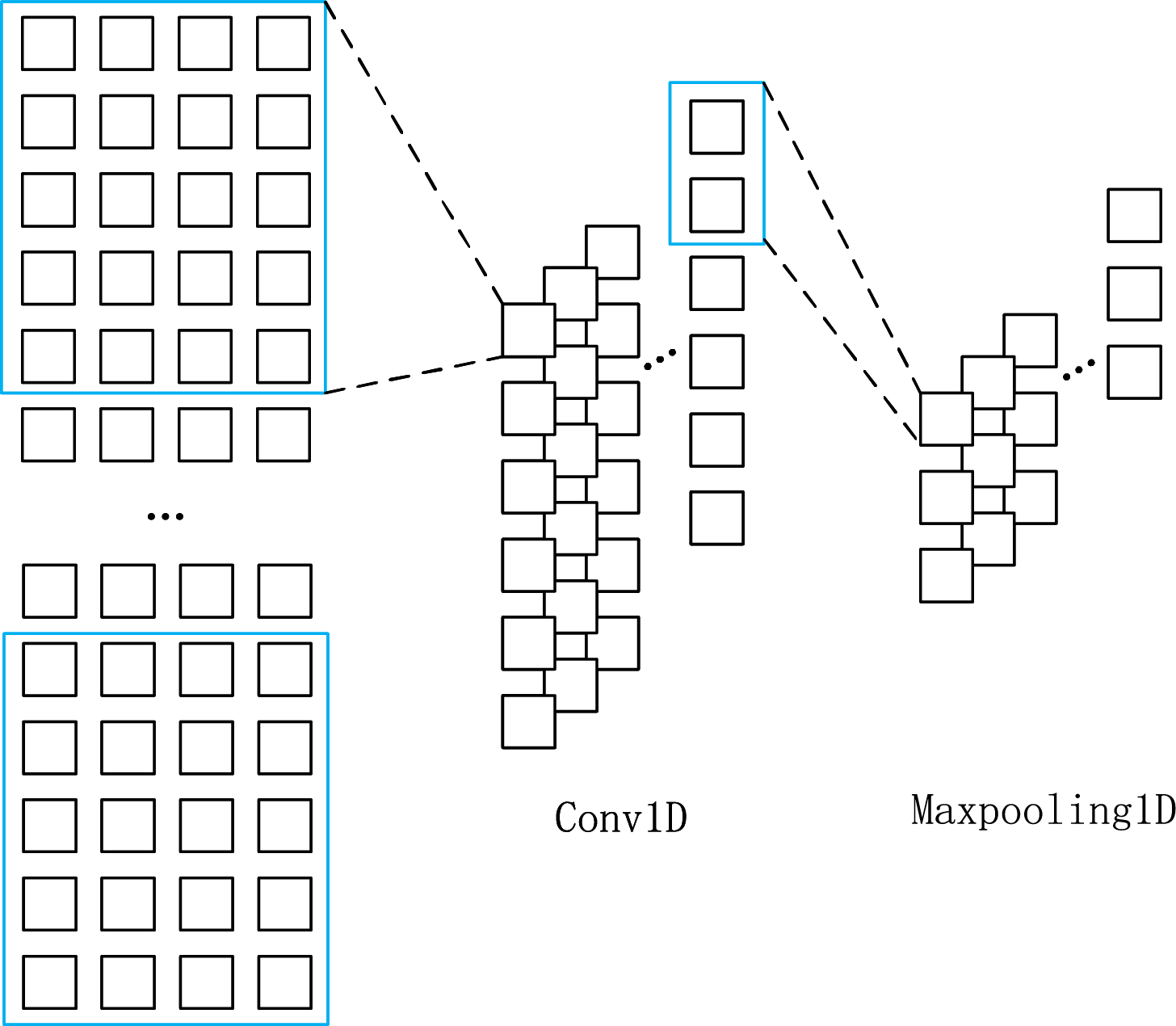
Figure 1: Schematic of the principles of 1DCNN and Maxpooling1D

3.2 LSTM

LSTM is a variant of Recurrent Neural Network (RNN), which implements information protection and control through three basic structures: forgetting gate (red rectangular part in Fig. 2), input gate (green rectangular part in Fig. 2), and output gate (yellow rectangular part in Fig. 2), and the principle schematic of LSTM is shown in the diagram of Fig. 2.

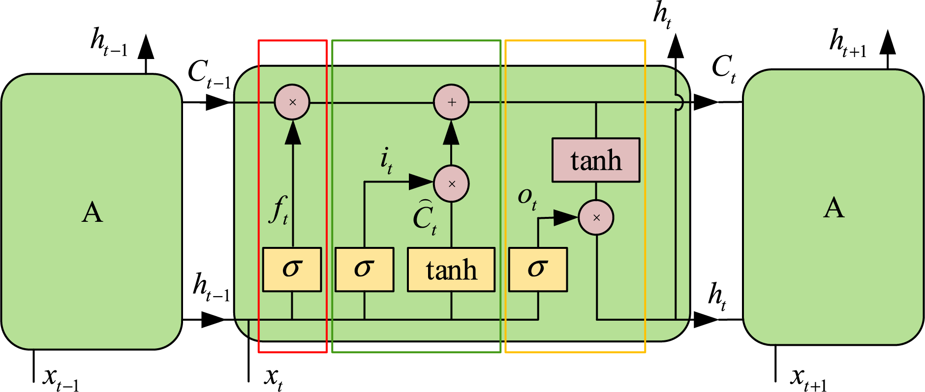
Figure 2: Schematic of the LSTM architecture in principle

How much information can be retained from the internal state Ct−1 at the previous moment is determined by the forgetting gate. How much information from the candidate state ⌢Ct can be retained at the current moment is determined by the input gate. How much information is output from the internal state Ct to the external state ht is determined by the output gate.

3.3 LSTM-1DCNN

Feature extraction is particularly crucial for HAR. To be able to extract temporal and spatial features of the measured data, we propose an LSTM-1DCNN algorithm that extracts temporal and spatial features in parallel through two branches; the structure of LSTM-1DCNN is shown in Fig. 3.

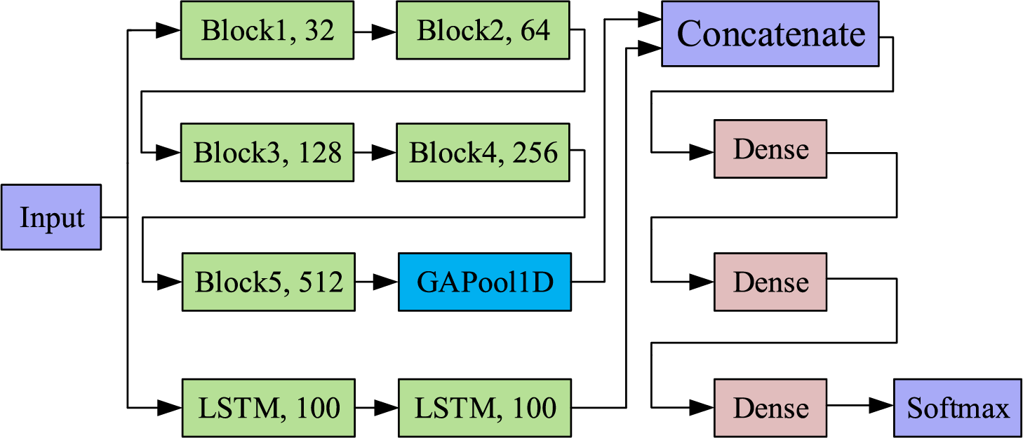
Figure 3: The principle schematic of LSTM-1DCNN

Each block of 1DCNN in Fig. 3 includes a convolutional layer, a batch normalization layer, an activation function, and a maximum pooling layer, the structure of which is shown schematically in Fig. 4.

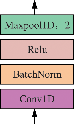
Figure 4: Block structure of 1DCNN

The first branch of the LSTM-1DCNN is the 1DCNN for extracting spatial features. This branch consists of a stack of five convolutional layers, pooling layers, etc. The pattern in the first branch is that the number of convolutional kernels is 32, 64, 128, 256, and 512, respectively, and the size of the convolutional kernels is kept constant at 9 for all. The 1DCNN branch constructed according to this schema allows the convolutional layer at the top of the algorithm to have a larger receptive field, which improves the ability of the algorithm for spatial feature extraction.

The second branch of LSTM-1DCNN is the LSTM for temporal feature extraction, which consists of two LSTM layers, both of which use 100 hidden layer nodes. The LSTM contains a mechanism to carry information across multiple time steps, allowing information to be saved for later use and thus preventing the problem of early signal fading during signal processing.

1DCNN and LSTM are two deep learning algorithms with completely different principles, which extract data features from a spatial and temporal perspective, respectively. The parallel connection of the two algorithms enables parallel extraction of spatio-temporal features, which are passed to the fully connected neural network after concatenation.

The spatial and temporal features contained in the data are equally relevant, and the temporal and spatial features obtained by LSTM-1DCNN are based on the following considerations.

Temporal features are those obtained by sequentially computing all samples in the measured data using an LSTM, which constructs a corresponding number of recurrent cells according to the number of samples and computes the samples according to their order. Each loop cell accepts the internal state and hidden layer state of the previous loop cell, as well as the information of the current sample, and selectively adds and forgets information to control the information accumulation rate. In this paper, we choose as output the hidden layer state of the last recurrent unit, which includes the information of all previous recurrent units and samples. Therefore, in this paper, we consider that LSTM is able to extract temporal features of measured data.

Spatial features are those obtained by the 1DCNN operating on an image composed of measurements. Unlike LSTM, 1DCNN does not consider the temporal relationship between two samples before and after convolution when using convolution kernels for feature extraction, and essentially operates the measured data as an image, so the extracted features are spatial. In this paper, we argue that 1DCNN can extract spatial features of measurement data by sliding convolution.

Overall, the features obtained by LSTM and 1DCNN do not have a similar clear physical meaning as those obtained by traditional feature engineering. However, the above understanding of temporal and spatial features in this paper has an unambiguous physical meaning.

The purpose of the proposed LSTM-1DCNN algorithm is to achieve the highest possible HAR performance when collecting data using a single triaxial accelerometer. Currently, some scholars use 1DCNN and LSTM to make a serial information fusion for HAR. However, we believe that serial processing of spatio-temporal information leads to information disorder since serial processing violates the physical relation between time and space. Therefore, in this paper, we propose parallel extraction of temporal and spatial features to obtain as much valid information as possible on raw measurement data and improve the recognition effect of HAR. This approach is more in line with the fundamental principles of joint temporal and spatial analysis and has further potential for development.

3.4 Data Pre-Processing

After data collection, the data needs to be preprocessed, which includes steps such as window partitioning, filtering, and data normalization. The data preprocessing procedure is shown in Fig. 5.

Figure 5: Pre-processing of the data

Currently, two types of time windows are commonly used in the field of HAR, one is a short time window of 1 to 3 s [33–36], and the other is a prolonged time window of 10 s or more [37,38], with the former being more commonly used. The study mentioned in reference [36] explores the impact of different sliding window lengths on evaluation metrics for classification algorithms, with a specific focus on the effect on F1-scores. Eight sliding window lengths ranging from 0.5 to 4 s with 0.5-s intervals were analyzed, and their effects on the evaluation metrics were examined. Experimental results show that when the window length is less than 3.5 s, the F1-score also increases with the window length. However, when the window length is larger than 3.5 s, the F1-score decreases as the window continues to increase. Therefore, literature suggests that results are better when the sliding window is 3 s, and that long or short time windows lead to a reduction in evaluation metrics.

Given the sampling frequency of the datasets used in this paper, we decided to use 2.56 s as the length of the sliding window, with a sliding window overlap rate of 50%. A schematic of the sliding window is shown in Fig. 6.

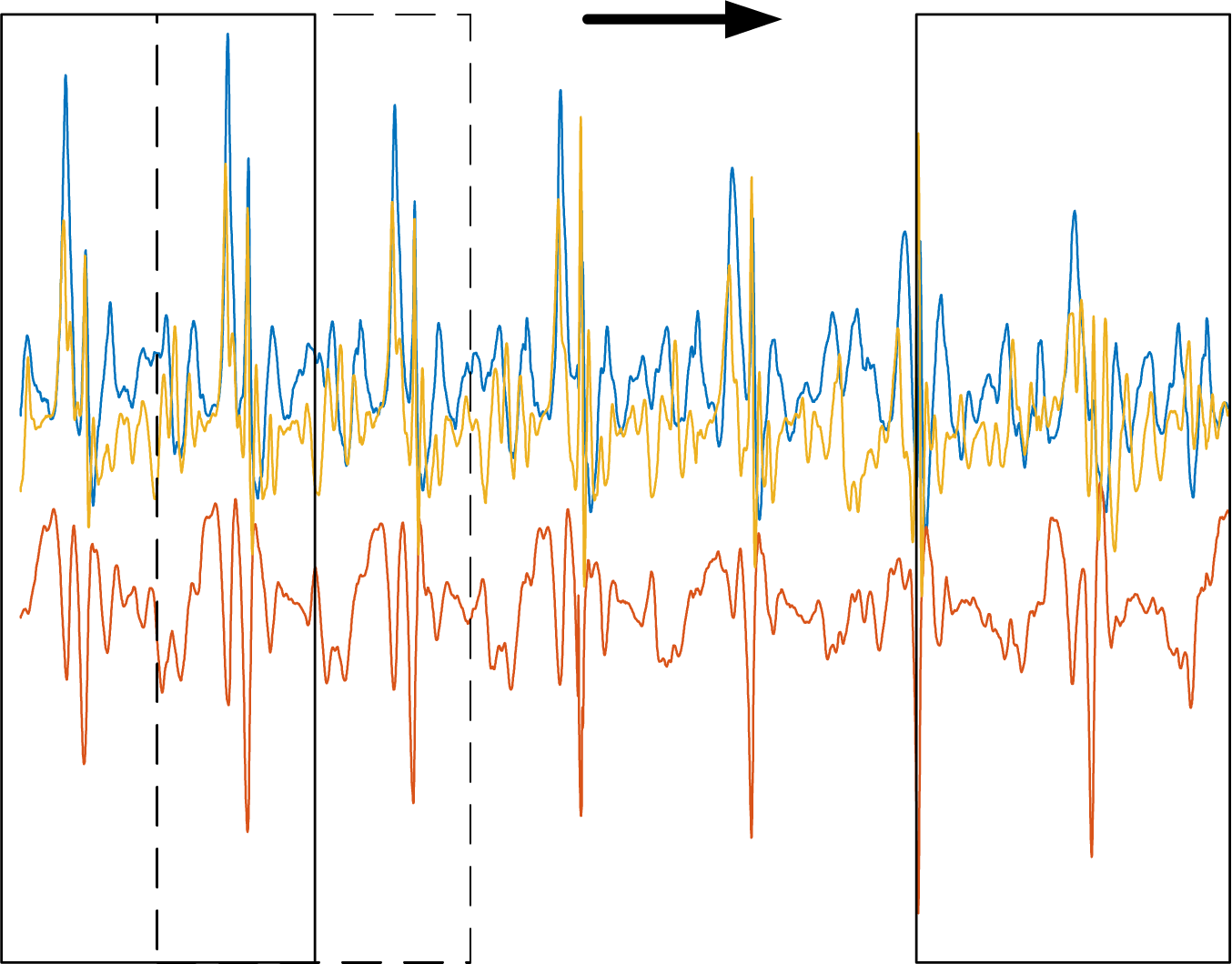
Figure 6: Schematic of a sliding window

Some algorithms are particularly sensitive to data normalization, such as neural networks and Support Vector Machine (SVM), while decision trees and random forests do not have a mandatory requirement. Considering that the algorithms used in this paper include multiple algorithms such as decision trees and SVM, which require normalization of the data, this paper uses max-min normalization to scale the data.

Various types of noise are unavoidable during data collection. Some scholars use filtering algorithms to minimize the contamination of the sampled data by noise as much as possible. Common filtering algorithms include sliding median filtering [19], mean filtering [35], and Butterworth low-pass filtering [39]. To suppress the effect of noise on the data, median filtering is used to reduce noise.

Normalization typically refers to the method of converting data features to the same scale, such as mapping data features to [0,1] or following a standard normal distribution with a mean of 0 and a variance of 1, etc. Common normalization methods include max-min normalization and standardization, among others. Some algorithms are extremely sensitive to data normalization, such as neural networks and SVM, while decision trees and random forests have no mandatory requirements. Considering that the algorithms used in this paper include multiple algorithms such as decision trees and SVM, which require normalization of the data, this paper uses max-min normalization to scale the data.

4  Experiments and Discussions

This section describes the following four aspects:

1.Basic information on the five publicly available datasets and the self-constructed dataset used in the experiments of this paper.

2. Performance of the proposed LSTM-1DCNN algorithm on various datasets.

3. Comparison of HAR performance of different algorithms and different scholars on publicly available datasets.

4. The deployment of the training results of the proposed LSTM-1DCNN algorithm proposed in this paper on Android phones.

4.1 Datasets

Human activity is extremely complex. When performing data collection on human activity, measurements can be affected by numerous factors. These influence factors include the sampling frequency of the sensor, the position of the fixation, the degree of fixation, and whether the activity of the experimenter is tightly constrained. The quality of the data itself can considerably affect the evaluation metrics of the recognition algorithms.

In order to evaluate the performance of the proposed LSTM-1DCNN algorithm, five commonly used public datasets in the field of HAR and a few self-built datasets are used for algorithm performance evaluation. The five publicly available datasets include: the UCI dataset [39], the WISDM dataset [40], the MotionSense dataset [41], the PAMAP2 dataset [42], and the MHEALTH dataset [43,44]. The basic information of the six datasets is described below.

The UCI dataset contains inertial measurements generated from 30 volunteers aged 19 to 48 who performed a total of six daily life activities: standing, sitting, lying, walking, going upstairs and downstairs. The inertial data were collected using a triaxial accelerometer and a triaxial gyroscope embedded in a smartphone (Samsung Galaxy SII) which is fixed to the volunteers’ waist. The sensors are sampled at 50 Hz to collect triaxial acceleration signals and triaxial angular velocity signals generated during human activity.

The WISDM dataset contains triaxial acceleration data from 36 volunteers performing activities that were collected in the categories of walking, jogging, walking upstairs, walking downstairs, sitting, and standing. To collect the data, the volunteers placed their smartphones in their trouser pockets and the sensors were sampled at 20 Hz to collect the triaxial acceleration signals generated by their activities.

The MotionSense dataset collected data from 24 volunteers of different genders, ages, weights, and heights for six activities, including walking upstairs and downstairs, walking, jogging, standing, and sitting under the same conditions. During data collection, all volunteers had their smartphones in their trouser pockets and the sensors were sampled at 50 Hz.

The PAMAP2 dataset collected acceleration data from 9 volunteers for 18 activity types. The dataset collected acceleration data from three different locations on the human body (chest, hand, and ankle) at a sampling frequency of 100 Hz.

The MHEALTH dataset collected acceleration data from 10 volunteers for 12 different activities. The types of activities included standing, sitting, cycling, and jogging. The dataset collected acceleration data of human activities at three locations (chest, right wrist, and left ankle) at a sampling frequency of 50 Hz.

The self-built dataset in this paper collected acceleration data from three volunteers for seven typical human activities. Activity types include sitting, standing, walking, lying, walking upstairs, walking downstairs, and running. The datasets were collected by mobile phones (HONOR V30Pro) in the volunteers’ trouser pockets using a sampling frequency of 50 Hz.

The problem studied in this paper is typical of HAR algorithms using a single triaxial accelerometer, but the aforementioned datasets contain measurements from multiple sensors, multiple mount locations, and multiple human activities. Therefore, these datasets were split and selected for use in this paper, with only a subset of the activity samples selected from the publicly available datasets. The data for some of the activities used in this paper are given in Table 1.

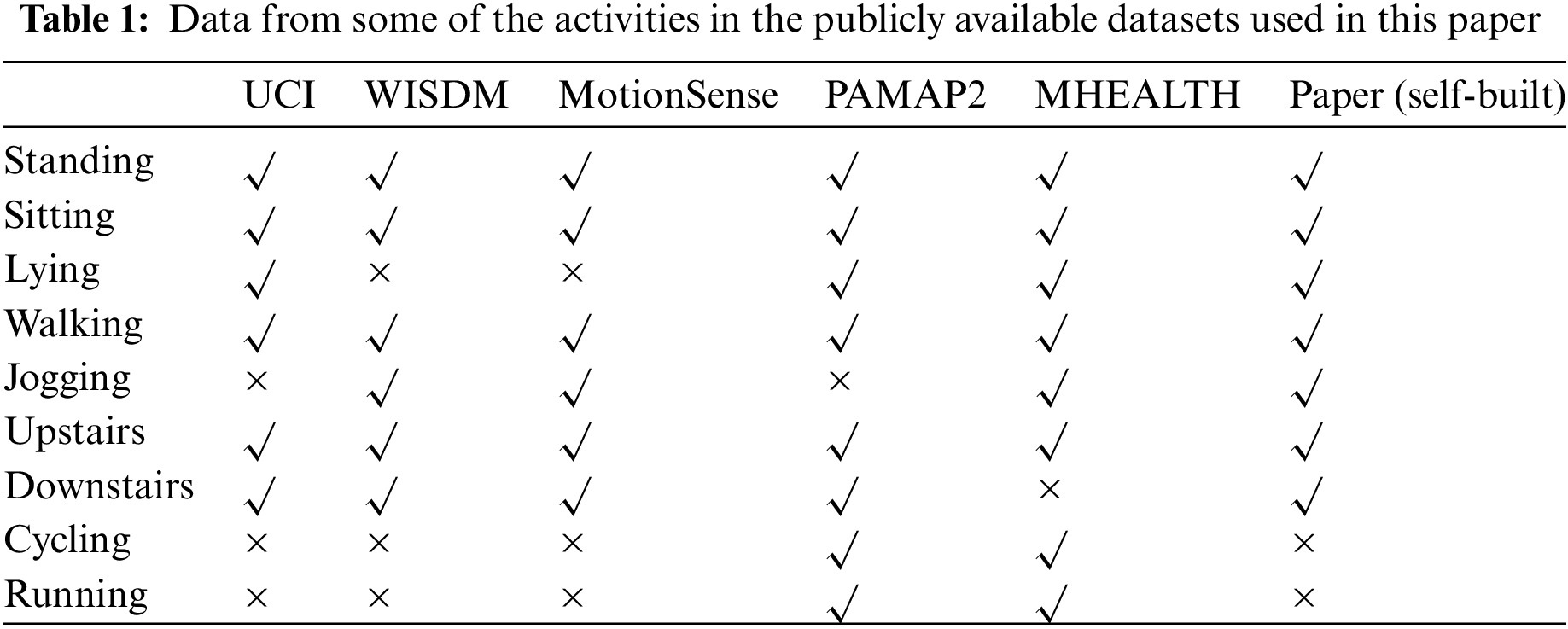
Of the six datasets mentioned above, UCI, WISDM, MotionSense, and the self-built dataset in this paper use a single body location to collect acceleration data. As the PAMAP2 and MHEALTH datasets use three body locations to collect acceleration data, a total of 10 body locations of acceleration data are available for training and evaluation. In Table 1, blanks with a check mark (√) indicate that the dataset contains the data of that activity and is used in this paper, and blanks with a cross mark (×) indicate that the dataset does not contain the data of that activity and is not used in this paper.

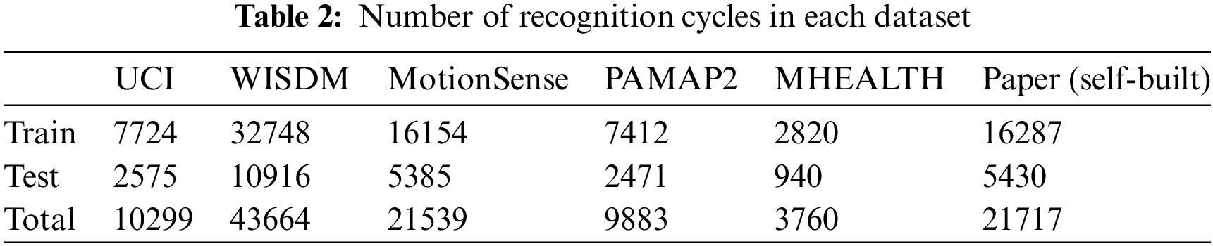
In this paper, the datasets are divided into several recognition cycles using a sliding window of length 2.56 s with a 50% overlap. The data are divided into training sets and test sets according to the 75% and 25% ratio. The number of samples is given in Table 2.

4.2 Evaluation Metrics

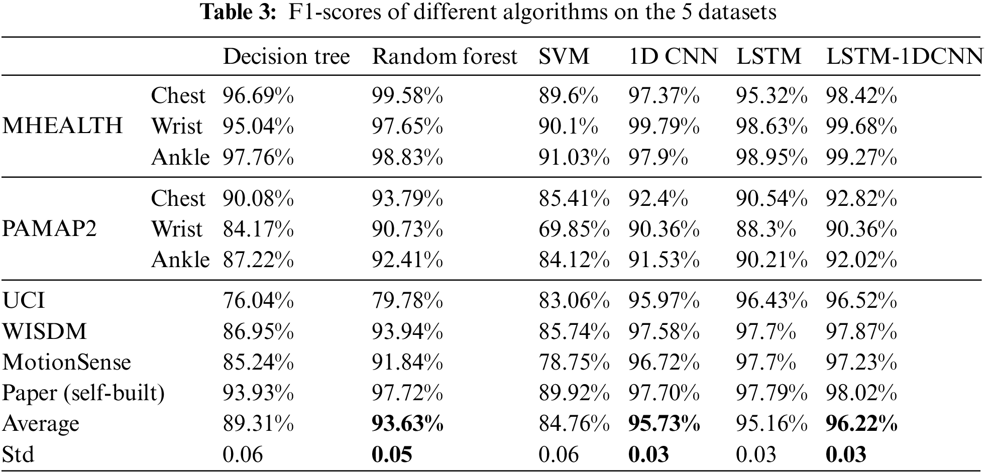
The numbers of samples in the HAR public datasets are different, and to accurately evaluate the HAR algorithm proposed in this paper, the macro-average F1-score was used in this paper as an evaluation metric, evaluation metrics for comparison between the LSTM-1DCNN in this paper and other common algorithms, as shown in Table 3.

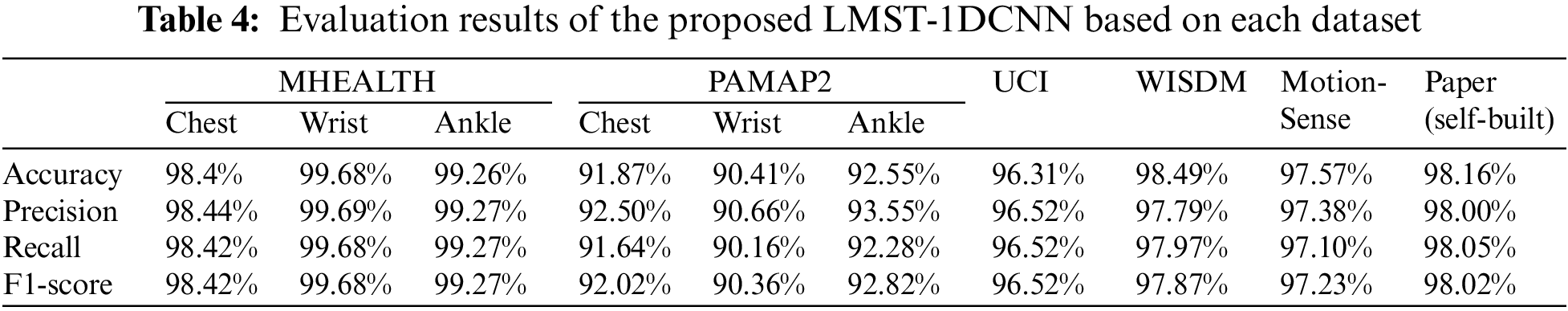
The average recognition rate, macro-average precision, macro-average recall, and macro-average F1-score (hereafter they refer to as Accuracy, Precision, Recall, and F1-socre) are used to evaluate the performance of the HAR algorithm constructed in this paper on several publicly available datasets, as shown in Table 4. These metrics are defined below.

Average recognition rate: the number of accurately predicted samples divided by the number of all samples. The formula is given in Eq. (1).

Accuracy=TP+TNTP+TN+FP+FN(1)

Precision: it describes how many of the samples predicted to be positive are positive. It is computed as in Eq. (2).

Precision=TPTP+FP(2)

Recall: it characterizes how many positive samples are predicted to be positive. It is computed as shown in Eq. (3).

Recall=TPTP+FN(3)

F1-score: harmonic mean of precision and recall. The formula for its computation is given in Eq. (4).

F1−score=2∗precision∗recallprecision+recall(4)

In the above equations, True Positive (TP) indicates the number of samples in which positive cases are predicted to be positive, True Negative (TN) indicates the number of samples in which negative cases are predicted to be negative, False Positive (FP) indicates the number of samples in which negative cases are predicted to be positive, and False Negative (FN) indicates the number of samples in which positive cases are predicted to be negative.

4.3 Experimental Analysis

All experiments were run on a Dell T640 workstation with a 24 GB NVIDIA RTX6000 video card and 256G RAM, and all algorithms were run on Python 3.6, Tensorflow 2.1.0, and Keras 2.3.1.

The algorithmic hyperparameters of LSTM-1DCNN are introduced in the order from the bottom layer to the top layer. The 1DCNN branch of LSTM-1DCNN uses a convolutional kernel size of 9, and the number of convolution kernel is 32, 64, 128, 256, and 512, respectively. The number of hidden layer nodes of the LSTM branch is 100. The number of hidden layer nodes of the fully connected neural network layer is 128, 64, 8, or 6, respectively (the number of hidden layer nodes of the fully connected neural network near the top layer depends on the type of activity in the dataset), the two fully connected neural network layers near the bottom use the Relu activation function, and the fully connected neural network layer near the top uses the Softmax activation function. The batch size of LSTM-1DCNN is 128, the number of iterations (epochs) is 240, the verification set proportion is 20%, the optimizer is Adam, and the learning rate reduction mechanism is used. The monitoring metric is set to val_loss, which decreases the learning rate when val_loss does not shift within 10 epochs.

4.3.1 Experimental Results

To enable a comprehensive evaluation of the LSTM-1DCNN algorithm, the LSTM-1DCNN is trained and evaluated on six datasets using the same algorithm structure and hyperparameters.

As shown in Table 4, the proposed LSTM-1DCNN algorithm is able to achieve excellent recognition results on six datasets. The F1-score on publicly available datasets ranges from 90.36% to 99.68%. The F1-score on the self-built dataset is 98.02%. Experimental results show that the evaluation metrics of the proposed LSTM-1DCNN algorithm significantly outperform the results of most known studies.

Table 4 shows that the PAMAP2 dataset has significantly lower evaluation metrics compared to the other four datasets. With the exception of the PAMPA2 dataset, the F1-score ranges from 96.52% to 99.68% for the other five datasets.

The most significant difference between PAMAP2 and the other four datasets was the sampling frequency of the sensors (As for other factors, we cannot confirm. For example, in the process of data collection, whether the activities of the experimenter are strictly regulated and whether the sensor is firmly fixed). The HAR research does not have a strict requirement for the sampling frequency of the sensors, so the sampling frequency used varies from dataset to dataset. For example, the sensor sampling frequency of the PAMAP2 dataset is 100 Hz, and the sampling frequencies of the other datasets are 20 and 50 Hz.

What difference will the different sampling frequencies make? For HAR algorithms, the division of the recognition period is a key step in the data processing, and different sampling frequencies lead to different numbers of samples within the same recognition period. We compared the different sampling frequencies through the following set of experiments, thereby verifying whether the sampling frequency of the PAMAP2 dataset is too high, which leads to the degradation of the evaluation metrics of the proposed LSTM-1DCNN.

In the following confirmation experiments, the sensor data of the PAMAP2 dataset are downsampled to obtain PAMAP2 with sampling frequencies of 20 and 50 Hz, and the proposed LSTM-1DCNN is trained and evaluated on the downsampled data. The evaluation results for the PAMAP2 dataset at different frequencies are shown in Table 5, and the F1-score pairs are shown in Fig. 7.

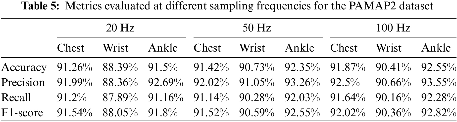
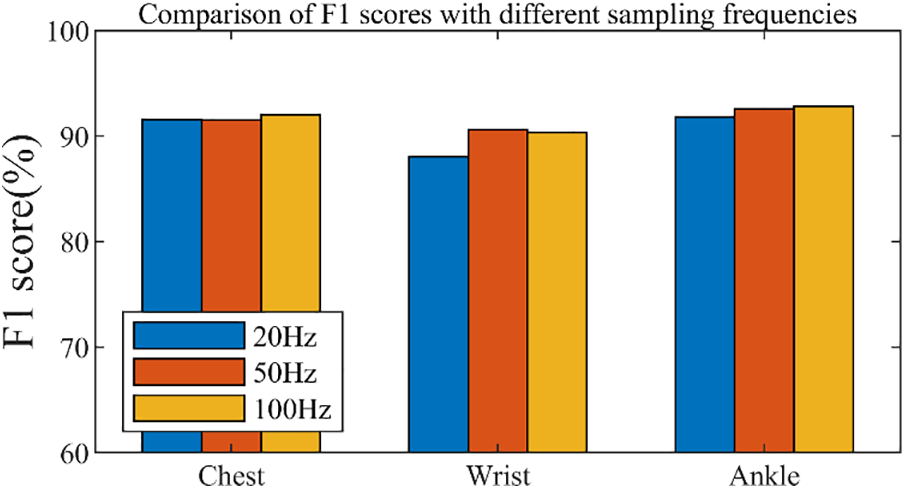
Figure 7: Comparison of F1-scores for different sampling frequencies

As shown in Table 5 and Fig. 7, there is no significant difference in the evaluation metrics using the proposed LSTM-1DCNN at the sampling frequencies of 20, 50, and 100 Hz. This indicates that for the proposed LSTM-1DCNN, the effect of sampling frequency on the recognition results is minor and does not lead to significant performance gains or losses. Therefore, the main difference between the PAMAP2 dataset and the others, namely the sampling frequency of 100 Hz, is not the main reason for its significantly lower evaluation metric. Since this phenomenon occurs only in the PAMPA2 dataset and is not consistent with the phenomenon shown in other datasets, it can be assumed that it is caused by some proprietary factor in the PAMPA2 dataset, which cannot be confirmed by some known factors.

4.3.2 Comparison Experiments

To compare the different performances of the proposed LSTM-1DCNN algorithm with other HAR algorithms, different algorithms are trained and evaluated on the same datasets in this section. The results of the comparison are shown in Table 3.

When comparing experiments using decision trees, random forests, and SVM, feature engineering of sensor measurements is required and then the features are given to the algorithm for training. In this paper, the X-axis, Y-axis, Z-axis, and the space vector’s amplitude of triaxial acceleration (Acc=Ax2+Ay2+Az2) are selected to extract 56 time-domain features. The extracted features include mean, variance, percentile, kurtosis and skewness, among others. It is expected that these time-domain features can characterize the differences between different activities and enhance the model performance.

Table 3 shows the evaluation metrics of different algorithms on different datasets. To facilitate the evaluation of the F1-score of different algorithms on different datasets, we calculate the mean and standard deviation of the F1-score of different algorithms on different datasets.

Based on the mean and standard deviation of the F1-score of the same algorithm on different datasets, it can be seen that the proposed LSTM-1DCNN algorithm performs the best with a mean of 96.22% and a standard deviation of 0.03. The highest mean and standard deviation of the F1-score of the three traditional machine learning algorithms on different datasets is 93.63% and 0.05, respectively. This shows that the performance robustness of the three traditional machine learning algorithms on different datasets is relatively poor. This paper argues that the fundamental reason for this situation is that all three machine learning algorithms require feature engineering, and it is difficult to ensure that the features designed by humans in feature engineering can identify the differences between different activities. However, what distinguishes deep learning from traditional machine learning is its ability to automatically extract features, which is the main reason why deep learning algorithms perform better than traditional machine learning algorithms.

When training and evaluating 1DCNN and LSTM on different datasets, the mean and standard deviation of the optimal F1-score are found to be 95.73% and 0.03, which is slightly worse than the evaluation metric of the LSTM-1DCNN algorithm. We conclude that the proposed LSTM-1DCNN, which can extract both temporal and spatial features, can outperform both 1DCNN and LSTM algorithms.

To facilitate a visual comparison of the performance differences between the different algorithms, Fig. 8 compares the F1-score of the different algorithms. As shown in, the F1-score of deep learning algorithms fluctuates considerably less than traditional machine learning algorithms. For example, the random forest algorithm achieves superior F1-score on the MHEALTH and PAMAP2 datasets, but lower F1-score on datasets such as UCI, and the performance fluctuates more across datasets. Deep learning algorithms can guarantee a steep F1-score on each dataset, with less fluctuation in performance across different datasets. Moreover, the comparison of the six algorithms shows that LSTM-1DCNN performs the best on the six datasets, achieving the highest mean F1-score and the lowest F1-score standard deviation.

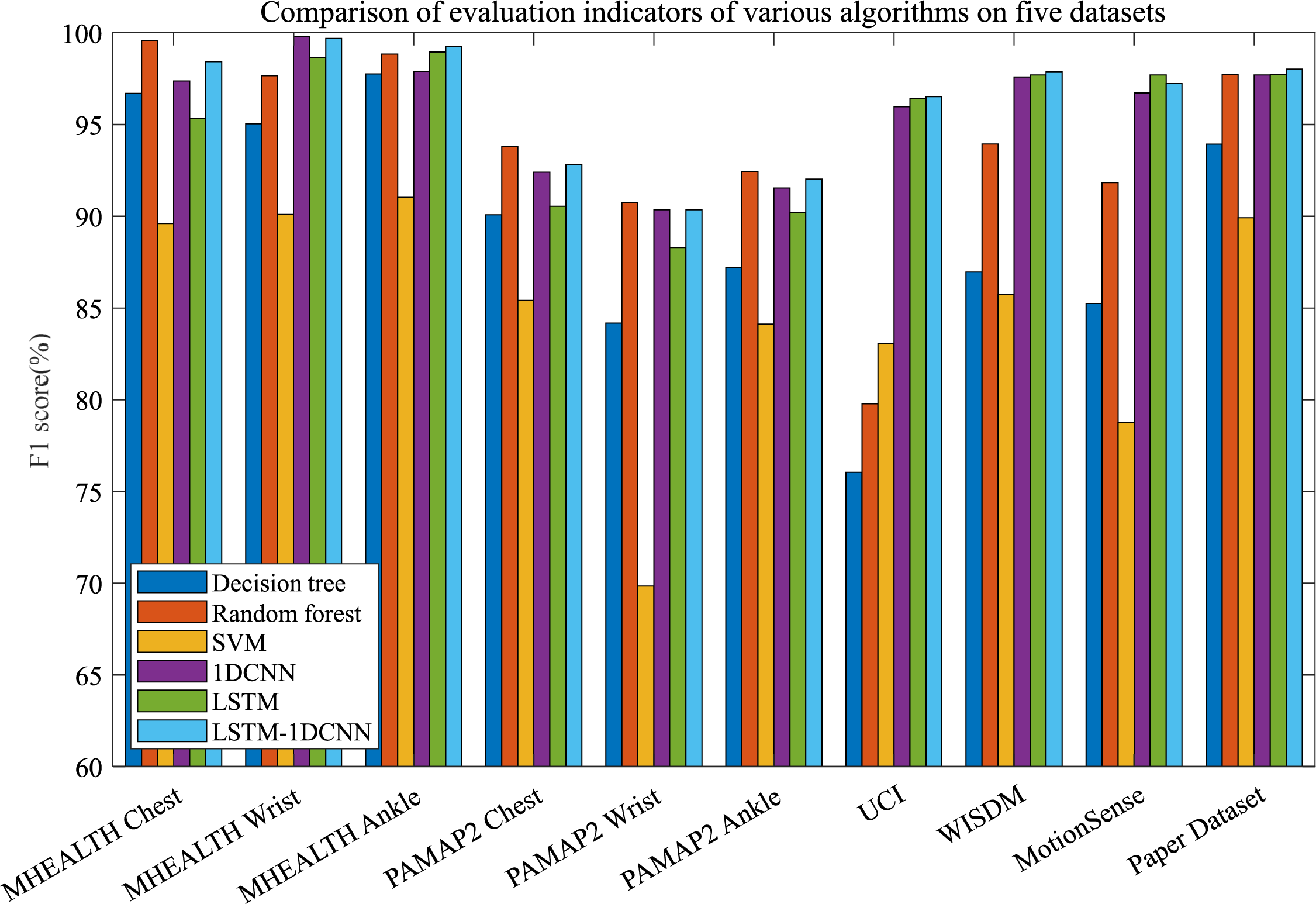
Figure 8: Comparison of evaluation metrics for various algorithms on six datasets

To compare with the results of different scholars in the field of HAR in recent years, Table 6 collects the recognition results of some scholars on five publicly available datasets. The proposed LSTM-1DCNN algorithm uses the same algorithmic structure and hyperparameters on different datasets. Under this premise, the performance of the proposed LSTM-1DCNN algorithm is at a strong level among peer studies. Therefore, it can be shown that the proposed LSTM-1DCNN algorithm is state-of-the-art and reasonable.

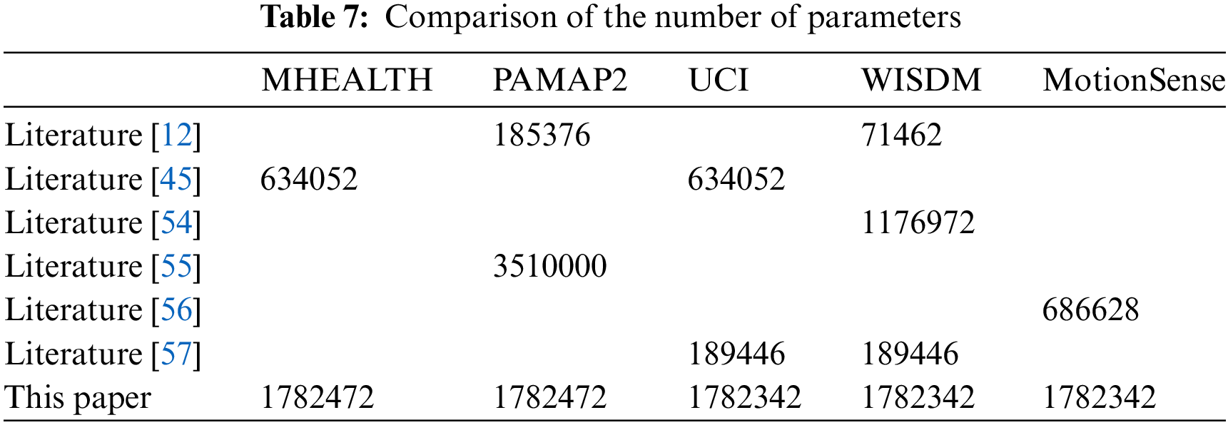
Different datasets contain different types of activities, which will affect the number of nodes in the fully connected layer near the top layer (the number of nodes is consistent with the number of classification categories), so that the number of algorithm parameters in different data sets is different, as shown in Table 7.

4.4 Model Deployment

Deployment of HAR algorithms is an influential part of HAR research. In this paper, model deployment is performed using the Simulink tool of Matrix Laboratory (MATLAB) software. MATLAB’s Simulink has a greatly powerful capability to generate Android programs for data acquisition and simple display of smartphone built-in sensors, so this paper only needs to consider the deployment of the forward computation process of our algorithm to smartphones.

The LSTM-1DCNN algorithm is first built using the MATLAB deep learning toolbox, where the structure and hyperparameters of the algorithm are the same as in the previous sections, and then re-trained and evaluated on a self-built dataset, after which the weights of each layer of the training results are saved.

The process of classifying a fresh set of measurements by the LSTM-1DCNN algorithm is the forward computation process of the LSTM-1DCNN, which is essentially the operation between the weight matrix of each layer of the algorithm and the measurements. The focus of the algorithm deployment is on how to implement the sampling of the data and the forward computation of the algorithm on the device.

In Simulink, the convolutional layer and pooling layer of the LSTM-1DCNN algorithm is firstly encapsulated into nine modules, and the trained weights are loaded in each module, and then the nine modules are called and connected several times according to the algorithm structure, to realize the forward computation process of LSTM-1DCNN algorithm, as shown in Fig. 9. Finally, the Android program is generated and deployed on a smartphone. The running interface of the Android program is shown in Fig. 10.

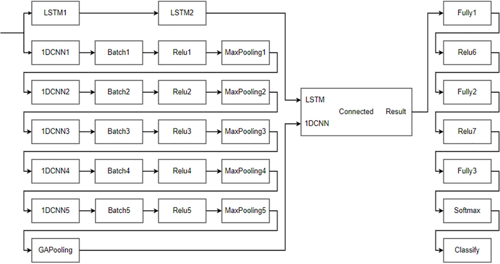
Figure 9: Structure of the LSTM-1DCNN algorithm in Simulink

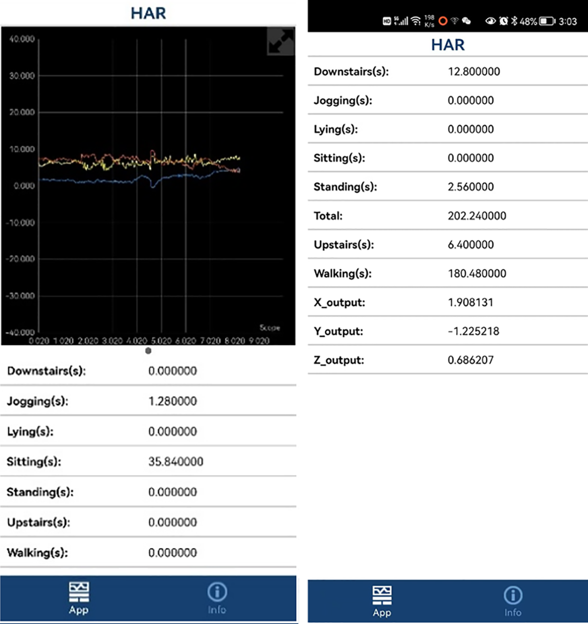
Figure 10: Deployment of LSTM-1DCNN on a smartphone

All previous algorithmic comparison works were implemented with Python programming, and the MATLAB platform was only used in the deployment work. To ensure that the deployment results are consistent with previous work, this paper compares two means of implementing the algorithm in Python and MATLAB. As shown in Table 8, both implementations have the same recognition rate.

In practice, the confusion matrix of HAR for mobile phone applications is shown in Table 9, and the evaluation metrics of the proposed LSTM-1DCNN algorithm are computed in Table 10.

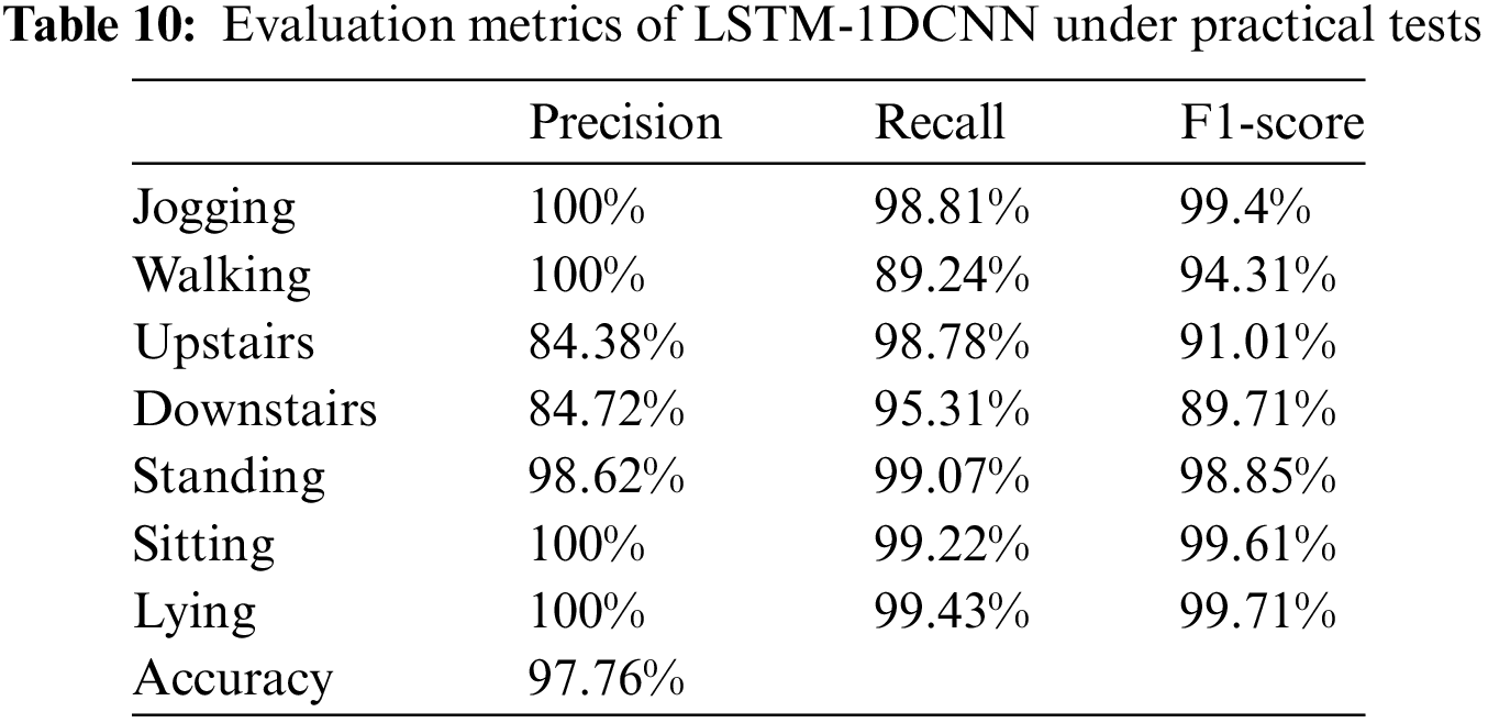
As can be seen from Table 10, in practice the accuracy is 84.38% for going upstairs, 84.72% for going downstairs, and 98.62% above for other activities. In addition, the F1-score for the downstairs was the lowest at 89.71%, while for the other activities it was above 91.01%. Therefore, the recognition rate of the proposed LSTM-1DCNN algorithm proposed in this paper to identify the above seven human activities is 97.76%. Therefore, it is reasonable to assume in this paper that this mobile application is capable of performing HAR accurately and that the deployment has achieved its intended goal.

5  Conclusions

In this paper, we propose an LSTM-1DCNN algorithm for HAR using a triaxial accelerometer. The algorithm contains two branches to extract both temporal and spatial features of the measured data. The algorithm is compared with five additional HAR algorithms (Decision Tree, Random Forest, Support Vector Machine, 1DCNN, and LSTM), and the algorithm is trained and evaluated on five publicly available datasets and self-built datasets. The evaluation metrics show that LSTM-1DCNN outperforms the remaining five algorithms in terms of recognition performance.

Moreover, the evaluation metrics of the LSTM-1DCNN algorithm are excellent when compared to related studies by other scholars. The reason for the excellent evaluation metric of LSTM-1DCNN is that the algorithm is able to extract both temporal and spatial features of the measured data and achieve joint temporal-spatial analysis.

To validate the performance of the LSTM-1DCNN algorithm in practice, the training results of the proposed algorithm are deployed in Android phones, and the actual tests show that the LSTM-1DCNN algorithm can accurately recognize seven typical human activities.

Currently, HAR is mainly performed on typical human activities, including walking, running, standing, sitting, lying, going upstairs, going downstairs, etc. The recognition of human events (falls, collisions, rollovers, etc.) and transitional activities (sitting to walking, walking to running, etc.) is expected but barely performed yet. Therefore, the LSTM-1DCNN algorithm will be applied to other HAR tasks.

In addition, the LSTM-1DCNN algorithm with joint temporal-space analysis capability can be applied to many additional domains, such as classification of sensor signals, mental state detection, physiological state detection, and mechanical vibration detection.

Acknowledgement: The authors warmly thank Dr. Wenhua Jiao for his great help.

Funding Statement: This work was supported by the Guangxi University of Science and Technology, Liuzhou, China, sponsored by the Researchers Supporting Project (No. XiaoKeBo21Z27, The Construction of Electronic Information Team supported by Artificial Intelligence Theory and Three-dimensional Visual Technology, Yuesheng Zhao). This work was supported by the 2022 Laboratory Fund Project of the Key Laboratory of Space-Based Integrated Information System (No. SpaceInfoNet20221120, Research on the Key Technologies of Intelligent Spatiotemporal Data Engine Based on Space-Based Information Network, Yuesheng Zhao). This work was supported by the 2023 Guangxi University Young and Middle-Aged Teachers’ Basic Scientific Research Ability Improvement Project (No. 2023KY0352, Research on the Recognition of Psychological Abnormalities in College Students Based on the Fusion of Pulse and EEG Techniques, Yutong Luo).

Author Contributions: Study conception and design: Yuesheng Zhao, Xiaoling Wang, Yutong Luo; Data collection: Xiaoling Wang, Yutong Luo; Analysis and interpretation of results: Yuesheng Zhao, Xiaoling Wang; Draft manuscript preparation: Xiaoling Wang, Yuesheng Zhao, Yutong Luo and Muhammad Shamrooz Aslam. All authors reviewed the results and approved the final version of the manuscript.

Availability of Data and Materials: The public datasets used in this study are accessible as described in references, they are the UCI dataset [39], the WISDM dataset [40], the MotionSense dataset [41], the PAMAP2 dataset [42], and the MHEALTH dataset [43,44]. Our self-built dataset can be accessed at the website: https://github.com/NBcaixukun/Human_activity_recognition_dataset.

Conflicts of Interest: The authors state that they have no conflicts of interest with respect to this study.

References

1. N. U. R. Malik, S. A. R. Abu-Bakar, U. U. Sheikh, A. Channa and N. Popescu, “Cascading pose features with CNN-LSTM for multiview human action recognition,” Sensors, vol. 4, no. 1, pp. 40–55, 2023. [Google Scholar]

2. Z. Hussain, Q. Z. Sheng and W. E. Zhang, “A review and categorization of techniques on device-free human activity recognition,” Journal of Network and Computer Applications, vol. 167, pp. 102738, 2020. [Google Scholar]

3. F. Kuncan, Y. Kaya and M. Kuncan, “New approaches based on local binary patterns for gender identification from sensor signals,” Journal of the Faculty of Engineering and Architecture of Gazi University, vol. 34, no. 4, pp. 2173–2185, 2019. [Google Scholar]

4. L. Chen, J. Hoey, C. D. Nugent, D. J. Cook and Z. Yu, “Sensor-based activity recognition,” IEEE Transactions on Systems, Man, and Cybernetics, Part C, vol. 42, no. 6, pp. 790–808, 2012. [Google Scholar]

5. L. Fan, Z. Wang and H. Wang, “Human activity recognition model based on decision tree,” in 2013 Int. Conf. on Advanced Cloud and Big Data, Nanjing, China, pp. 64–68, 2013. [Google Scholar]

6. A. Saha, T. Sharma, H. Batra, A. Jain and V. Pal, “Human action recognition using smartphone sensors,” in 2020 Int. Conf. on Computational Performance Evaluation, Shillong, India, pp. 238–243, 2020. [Google Scholar]

7. O. C. Kurban and T. Yıldırım, “Daily motion recognition system by a triaxial accelerometer usable in different positions,” IEEE Sensors Journal, vol. 19, no. 17, pp. 7543–7552, 2019. [Google Scholar]

8. I. A. Lawal and S. Bano, “Deep human activity recognition with localization of wearable sensors,” IEEE Access, vol. 8, pp. 155060–155070, 2020. [Google Scholar]

9. Z. Xiao, X. Xu, H. Xing, F. Song, X. Wang et al., “A federated learning system with enhanced feature extraction for human activity recognition,” Knowledge-Based Systems, vol. 229, no. 5, pp. 107338, 2021. [Google Scholar]

10. R. Kanjilal and I. Uysal, “The future of human activity recognition: Deep learning or feature engineering?” Neural Processing Letters, vol. 53, no. 1, pp. 561–579, 2021. [Google Scholar]

11. T. Liu, S. Wang, Y. Liu, W. Quan and L. Zhang, “A lightweight neural network framework using linear grouped convolution for human activity recognition on mobile devices,” The Journal of Supercomputing, vol. 78, no. 5, pp. 6696–6716, 2022. [Google Scholar]

12. Y. Li and L. Wang, “Human activity recognition based on residual network and BiLSTM,” Sensors, vol. 22, no. 2, pp. 635, 2022. [Google Scholar] [PubMed]

13. P. Sa-nguannarm, E. Elbasani, B. Kim, E. H. Kim and J. D. Kim, “Experimentation of human activity recognition by using accelerometer data based on LSTM,” Advanced Multimedia and Ubiquitous Engineering, vol. 716, pp. 83–89, 2021. [Google Scholar]

14. X. X. Han, J. Ye and H. Y. Zhou, “Data fusion-based convolutional neural network approach for human activity recognition,” Computer Engineering and Design, vol. 41, no. 2, pp. 522–528, 2020. [Google Scholar]

15. S. Z. Deng, B. T. Wang, C. G. Yang and G. R. Wang, “Convolutional neural networks for human activity recognition using multi-location wearable sensors,” Journal of Software, vol. 30, no. 3, pp. 718–737, 2019. [Google Scholar]

16. R. Kanjilal and I. Uysal, “Rich learning representations for human activity recognition: How to empower deep feature learning for biological time series,” Journal of Biomedical Informatics, vol. 134, pp. 104180, 2022. [Google Scholar] [PubMed]

17. X. Y. Chen, T. R. Zhang, X. F. Zhu and L. F. Mo, “Human behavior recognition method based on fusion model,” Transducer and Microsystem Technologies, vol. 40, no. 1, pp. 136–139+143, 2021. [Google Scholar]

18. J. Jiang and Y. F. Li, “Lightweight CNN activity recognition algorithm,” Journal of Chinese Computer Systems, vol. 40, no. 9, pp. 1962–1967, 2019. [Google Scholar]

19. J. He, Z. L. Guo, L. Y. Liu and Y. H. Su, “Human activity recognition technology based on sliding window and convolutional neural network,” Journal of Electronics & Information Technology, vol. 44, no. 1, pp. 168–177, 2022. [Google Scholar]

20. V. Ghate, “Hybrid deep learning approaches for smartphone sensor-based human activity recognition,” Multimedia Tools and Applications, vol. 80, no. 28, pp. 35585–35604, 2021. [Google Scholar]

21. M. M. Hassan, M. Z. Uddin, A. Mohamed and A. Almogren, “A robust human activity recognition system using smartphone sensors and deep learning,” Future Generation Computer Systems, vol. 81, pp. 307–313, 2018. [Google Scholar]

22. S. Mekruksavanich, A. Jitpattanakul and P. Thongkum, “Placement effect of motion sensors for human activity recognition using LSTM network,” in 2021 Joint Int. Conf. on Digital Arts, Media and Technology with ECTI Northern Section Conf. on Electrical, Electronics, Computer and Telecommunication Engineering, Cha-am, Thailand, pp. 273–276, 2021. [Google Scholar]

23. K. Wang, J. He and L. Zhang, “Attention-based convolutional neural network for weakly labeled human activities’ recognition with wearable sensors,” IEEE Sensors Journal, vol. 19, no. 17, pp. 7598–7604, 2019. [Google Scholar]

24. X. R. Song, X. Q. Zhang, Z. Zhang, X. H. Chen and H. W. Liu, “Muti-sensor data fusion for complex human activity recognition,” Journal of Tsinghua University (Science and Technology), vol. 60, no. 10, pp. 814–821, 2020 (In Chinese). [Google Scholar]

25. R. Mutegeki and D. S. Han, “A CNN-LSTM approach to human activity recognition,” in 2020 Int. Conf. on Artificial Intelligence in Information and Communication, Fukuoka, Japan, pp. 362–366, 2020. [Google Scholar]

26. S. Bohra, V. Naik and V. Yeligar, “Towards putting deep learning on the wrist for accurate human activity recognition,” in 2021 IEEE Int. Conf. on Pervasive Computing and Communications Workshops and other Affiliated Events, Kassel, KS, Germany, pp. 605–610, 2021. [Google Scholar]

27. N. T. H. Thu and D. S. Han, “HiHAR: A hierarchical hybrid deep learning architecture for wearable sensor-based human activity recognition,” IEEE Access, vol. 9, pp. 145271–145281, 2021. [Google Scholar]

28. S. A. Syed, D. Sierra-Sosa, A. Kumar and A. Elmaghraby, “A deep convolutional neural network-XGB for direction and severity aware fall detection and activity recognition,” Sensors, vol. 22, no. 7, pp. 2547, 2022. [Google Scholar] [PubMed]

29. Y. Li, S. Zhang, B. Zhu and W. Wang, “Accurate human activity recognition with multi-task learning,” CCF Transactions on Pervasive Computing and Interaction, vol. 2, no. 4, pp. 288–298, 2020. [Google Scholar]

30. N. Dua, S. N. Singh and V. B. Semwal, “Multi-input CNN-GRU based human activity recognition using wearable sensors,” Computing, vol. 103, no. 7, pp. 1461–1478, 2021. [Google Scholar]

31. G. Zheng, “A novel attention-based convolution neural network for human activity recognition,” IEEE Sensors Journal, vol. 21, no. 23, pp. 27015–27025, 2021. [Google Scholar]

32. C. T. Yen, J. X. Liao and Y. K. Huang, “Feature fusion of a deep-learning algorithm into wearable sensor devices for human activity recognition,” Sensors, vol. 21, no. 24, pp. 8294, 2021. [Google Scholar] [PubMed]

33. J. Wang, K. Zhang and Y. Zhao, “Human activities recognition by intelligent calculation under appropriate prior knowledge,” in Proc. of 2021 5th Asian Conf. on Artificial Intelligence Technology (ACAIT), Haikou, China, pp. 690–696, 2021. [Google Scholar]

34. J. Wang, K. Zhang, Y. Zhao and M. S. Aslam, “Cascade human activities recognition based on simple intelligent calculation with appropriate prior knowledge,” Computers, Materials & Continua, vol. 77, no. 1, pp. 79–96, 2023. [Google Scholar]

35. X. Jia, E. Wang and J. Wu, “Real-time human behavior recognition based on android platform,” Computer Engineering and Applications, vol. 54, no. 24, pp. 164–167+175, 2018. [Google Scholar]

36. M. Lv, W. Chen, T. Chen and Y. Liu, “Human activity recognition based on grouped residuals combined with spatial learning,” Journal of Zhejiang University of Technology, vol. 49, no. 2, pp. 215–224, 2021. [Google Scholar]

37. S. M. Lee, S. M. Yoon and H. Cho, “Human activity recognition from accelerometer data using convolutional neural network,” in 2017 IEEE Int. Conf. on Big Data and Smart Computing, Jeju, Korea, pp. 131–134, 2017. [Google Scholar]

38. D. Garcia-Gonzalez, D. Rivero, E. Fernandez-Blanco and R. Miguel, “A public domain dataset for real-life human activity recognition using smartphone sensors,” Sensors, vol. 20, no. 8, pp. 7853, 2021. [Google Scholar]

39. D. Anguita, A. Ghio, L. Oneto, X. Parra Perez and J. L. Reyes Ortiz, “A public domain dataset for human activity recognition using smartphones,” in 21th European Symp. on Artificial Neural Networks, Computational Intelligence and Machine Learning, Bruges, Belgium, pp. 437–442, 2013. [Google Scholar]

40. J. R. Kwapisz, G. M. Weiss and S. A. Moore, “Activity recognition using cell phone accelerometers,” ACM SigKDD Explorations Newsletter, vol. 12, no. 2, pp. 74–82, 2011. [Google Scholar]

41. M. Malekzadeh, R. G. Clegg, A. Cavallaro and H. Haddadi, “Mobile sensor data anonymization,” in 2019. Mobile Sensor Data Anonymization. In Proc. of the Int. Conf. on Internet of Things Design and Implementation, Montreal, Canada, pp. 49–58, 2019. [Google Scholar]

42. A. Reiss and D. Stricker, “Introducing a new benchmarked dataset for activity monitoring,” in The 16th IEEE Int. Symp. on Wearable Computers, Newcastle, UK, pp. 108–109, 2012. [Google Scholar]

43. O. Banos, R. Garcia, J. A. Holgado-Terriza, M. Damas, H. Pomares et al., “mHealthDroid: A novel framework for agile development of mobile health applications,” in Proc. of the 6th Int. Work-Conf. on Ambient Assisted Living an Active Ageing, Belfast, UK, pp. 91–98, 2014. [Google Scholar]

44. O. Banos, C. Villalonga, R. Garcia, A. Saez, M. Damas et al., “Design, implementation and validation of a novel open framework for agile development of mobile health applications,” Biomedical Engineering Online, vol. 14, no. 2, pp. 1–20, 2015. [Google Scholar]

45. M. A. Khatun, M. A. Yousuf, S. Ahmed, M. Z. Uddin, S. A. Alyami et al., “Deep CNN-LSTM with self-attention model for human activity recognition using wearable sensor,” IEEE Journal of Translational Engineering in Health and Medicine, vol. 10, pp. 2700316, 2022. [Google Scholar] [PubMed]

46. J. O'halloran and E. Curry, “A comparison of deep learning models in human activity recognition and behavioural prediction on the MHEALTH dataset,” in Irish Conf. on Artificial Intelligence and Cognitive Science, Wuhan, CN, pp. 212–223, 2019. [Google Scholar]

47. A. K. M. Masum, M. E. Hossain, A. Humayra, S. Islam, A. Barua et al., “A statistical and deep learning approach for human activity recognition,” in 3rd Int. Conf. on Trends in Electronics and Informatics, Tirunelveli, Tamil Nadu, India, pp. 1332–1337,2019, 2019. [Google Scholar]

48. S. Wan, L. Qi, X. Xu, C. Tong and Z. Gu, “Deep learning models for real-time human activity recognition with smartphones,” Mobile Networks and Applications, vol. 25, no. 2, pp. 743–755, 2020. [Google Scholar]

49. M. Gil-Martín, R. San-Segundo, F. Fernández-Martínez and R. de Córdoba, “Human activity recognition adapted to the type of movement,” Computers & Electrical Engineering, vol. 88, pp. 106822, 2020. [Google Scholar]

50. M. Gochoo, S. B. U. D. Tahir, A. Jalal and K. Kim, “Monitoring real-time personal locomotion behaviors over smart indoor-outdoor environments via body-worn sensors,” IEEE Access, vol. 9, pp. 70556–70570, 2021. [Google Scholar]

51. S. B. U. D. Tahir, A. B. Dogar, R. Fatima, A. Yasin, M. Shafig et al., “Stochastic recognition of human physical activities via augmented feature descriptors and random forest model,” Sensors, vol. 22, no. 17, pp. 6632, 2022. [Google Scholar] [PubMed]

52. A. Sharshar, A. Fayez, Y. Ashraf and W. Gomaa, “Activity with gender recognition using accelerometer and gyroscope,” in 2021 15th Int. Conf. on Ubiquitous Information Management and Communication, Seoul, Korea, pp. 1–7, 2021. [Google Scholar]

53. N. Halim, “Stochastic recognition of human daily activities via hybrid descriptors and random forest using wearable sensors,” Array, vol. 15, pp. 100190, 2022. [Google Scholar]

54. T. T. Alemayoh, J. H. Lee and S. Okamoto, “New sensor data structuring for deeper feature extraction in human activity recognition,” Sensors, vol. 21, no. 8, pp. 2814, 2021. [Google Scholar] [PubMed]

55. W. Gao, L. Zhang, Q. Teng, J. He and H. Wu, “DanHAR: Dual attention network for multimodal human activity recognition using wearable sensors,” Applied Soft Computing, vol. 111, pp. 107728, 2021. [Google Scholar]

56. M. Jaberi and R. Ravanmehr, “Human activity recognition via wearable devices using enhanced ternary weight convolutional neural network,” Pervasive and Mobile Computing, vol. 83, pp. 101620, 2022. [Google Scholar]

57. K. Suwannarat and W. Kurdthongmee, “Optimization of deep neural network-based human activity recognition for a wearable device,” Heliyon, vol. 7, no. 8, pp. e07797, 2021. [Google Scholar] [PubMed]