Strengthening Network Security: Deep Learning Models for Intrusion Detection with Optimized Feature Subset and Effective Imbalance Handling

1  Introduction

With the rapid development of Internet technology, there has been an increase in network attacks, drawing significant attention to network security [1]. The main objective of cyber attacks is to tamper with or steal sensitive data. Network attacks are classified into active attacks and passive attacks. Active attacks compromise system integrity and availability, while passive attacks involve hackers collecting system information by scanning open ports and vulnerabilities [2–4]. Intrusion detection systems serve as an active defense mechanism by capturing network traffic packets and analyzing them, ensuring the security of computer systems [5].

Since Denning [6] introduced the first intrusion detection system, many methods have been used in the field of network security. According to recent research, mainstream IDSs are primarily divided into two parts. The first part involves data preprocessing, including feature engineering and handling data set imbalances. The second part entails the construction of classifiers.

On the other hand, intrusion detection typically faces two scenarios. In the first scenario, regression-based machine learning methods can be used for intrusion detection and prevention by analyzing changes in network parameters. For example, historical network data and related intrusion data can be used for training to build a regression model for predicting changes in network parameters (e.g., k-barrier [7]). By monitoring real-time network data and comparing it with the predicted results, potential intrusion behaviors can be detected promptly, and appropriate preventive measures can be taken, such as blocking abnormal network connections or notifying system administrators.

In the second scenario, machine learning is primarily used for intrusion classification. Intrusion classification is a supervised learning problem that requires training with known intrusion samples to establish a classification model that can categorize input data into different intrusion categories. These intrusion categories may include network scans, malware, denial of service attacks, and more. Once trained, this model can be used for real-time monitoring of traffic in systems and networks, categorizing it as normal behavior or potential intrusion behavior for timely response. To enhance the accuracy of intrusion detection, various machine learning algorithms such as decision trees, support vector machines, random forests, and more can be utilized. Furthermore, techniques like feature selection, data preprocessing, and ensemble learning can be employed to further improve the performance of intrusion detection systems. This paper focuses on the second scenario.

In recent years, machine learning methods have seen rapid development and have become the mainstream technology in intrusion detection. Machine learning-based intrusion detection systems face four challenges that affect the performance of model detection. These challenges include high data dimensionality with a large number of redundant features, data set imbalances, insufficient feature extraction by classifiers, and classifier hyperparameter issues.

Feature engineering plays a crucial role in reducing dimensionality, training time, and computational costs associated with dataset features, while also enhancing model performance [8]. Redundant features within the dataset can cause overfitting during the learning process, resulting in reduced detection performance of the model [9]. To address the issue of feature redundancy, feature selection is deemed as the optimal solution. Feature selection involves selecting the most appropriate subset of features from the dataset to facilitate more effective model training. There are two primary approaches to feature selection: filters and wrappers. The filter approach utilizes variable ranking techniques to rank the feature variables, irrespective of the classifier type, and removes irrelevant variables by applying predefined thresholds [10]. On the other hand, the wrapper approach relies on a classifier and leverages its predictions to select the most relevant subset of features.

Intrusion detection research often relies on laboratory datasets. However, these datasets often suffer from data imbalance issues in accurately representing real-world network traffic. Typically, the number of normal network traffic instances in the dataset far surpasses the instances of attack traffic belonging to specific categories. Classifiers trained on unbalanced datasets may struggle to identify minority classes. Therefore, most researchers employ resampling techniques to balance the dataset [11]. However, oversampling and undersampling can lead to overfitting or underfitting problems during model training.

Network attacks against Internet devices occur frequently, and network attack methods are constantly updated and upgraded, adding significant detection pressure to intrusion detection systems. Traditional machine learning-based technologies, such as k-Nearest Neighbors and Naïve Bayes, are no longer capable [12]. Deep learning technology has shown promise in effectively detecting complex and evolving network attacks. However, it still faces challenges, such as insufficient feature extraction from network traffic [13,14].

To address these challenges, this paper proposes four deep neural network models: Multi-Conv1d, Multi-Conv1d-Self-attention, Mulit-Conv1d-BiLSTM-Attenion, and Mulit-Conv1d-BiGRU-Attention. These models fully extract network traffic characteristics and effectively detect various types of network attacks. They specialize in extracting either spatial or spatio-temporal features from network traffic data, focusing on key features. Additionally, to tackle the class imbalance problem, we incorporate focal loss to adjust instance weights, making the model concentrate on difficult-to-classify samples and improving the detection rate of minority classes.

The main contributions of this paper are as follows:

1. Dimensionality reduction and feature selection using the particle swarm optimization algorithm to enhance model accuracy, generalization, and running speed.

2. Proposal of four deep learning models that efficiently detect network attacks. Multi-Conv1d, BiLSTM (BiGRU), and Attention mechanisms are combined to extract spatial and temporal characteristics of network traffic. Attention guidance is employed to prioritize key feature information, thereby improving model performance and achieving efficient detection.

3. Hyperparameter optimization techniques are employed to achieve the highest model performance.

4. Utilization of focal loss function for training the neural network model, addressing the data set’s imbalance problem.

5. Evaluation of the proposed models on the NSL-KDD dataset, demonstrating superior results in binary and multi-class experiments compared to other state-of-the-art methods.

The remainder of this article is organized as follows: Section 2 introduces relevant literature on intrusion detection; Section 3 presents our proposed method; Section 4 describes the experimental setup and analysis; and finally, Section 5 summarizes our work.

2  Related Works

With the rapid development of machine learning, it is widely used in the field of intrusion detection to protect the security of computer networks. Some researchers have utilized classical machine learning algorithms such as RF, SVM, Naïve Bayes (NB), and DT for intrusion detection [15]. Furthermore, deep learning algorithms such as CNN and RNN have also been applied in this domain [15].This section provides a review of recent literature pertaining to intrusion detection.

Malibari et al. [16] proposed a novel intrusion detection system. They began by preprocessing the data using Z-score normalization, employed an improved arithmetic optimization algorithm for dimensionality reduction and feature selection, used the deep wavelet neural network (DWNN) model as the foundational classifier, and finally optimized the model’s parameters using quantum behaved particle swarm optimization (QPSO). Experimental validation was conducted on the CIC-IDS2017 dataset, and the results demonstrated that the proposed approach outperformed other state-of-the-art methods.

Murali Mohan et al. [17] introduced a new intrusion detection system for cloud environments. It is primarily divided into four stages: data preprocessing, optimal clustering, feature selection, and attack detection. They utilized an optimized Deep Belief Network (DBN) to detect attack types and fine-tuned the DBN using a new hybrid optimization model (SMSLO). In the validation phase, excellent results were achieved.

Sukumar et al. [18] introduced an efficient intrusion detection system that utilizes the Improved Genetic K-means (IGKM) algorithm for detecting attack traffic. Experimental findings demonstrate that the K-means clustering algorithm achieves higher accuracy when applied to larger datasets.

Kasongo et al. [19] employed a feature selection method based on XGBoost to mitigate the impact of high-dimensional data on IDS detection performance. By selecting 19 optimal features, the decision tree (DT) achieved a 2.72% improvement in test accuracy for binary classification.

Ustebay et al. [20] used a random forest classifier combined with recursive feature elimination to reduce dataset dimensionality and efficiently detect attack traffic in computer networks. Through experiments conducted on the CIC-IDS2017 dataset, using a Deep Multilayer Perceptron as a classifier, they achieved an accuracy rate of 91%.

Wu et al. [21] proposed a novel hybrid sampling method to address the issue of detection result inaccuracies caused by data imbalance. The K-means clustering algorithm and the SMOTE algorithm were utilized to balance the dataset. Experiments on the NSL-KDD dataset showed that when enhanced random forest was used as a classifier, the training and test set achieved accuracy rates of 99.72% and 78.47%, respectively.

Man et al. [22] introduced a network intrusion detection model based on residual blocks to tackle the diminishing detection performance as the number of layers increased in deep neural network-based intrusion detection systems. By converting network traffic into images and utilizing residual blocks to construct a deep convolutional neural network, they achieved high performance on the UNSW-NB15 dataset.

El-Ghamry et al. [15] aimed to safeguard the network security of intelligent agricultural equipment. They utilized recursive feature elimination to select important features, converted network traffic into color images, and inputted them into models such as VGG, Inception, and Xception while optimizing the hyperparameters using the PSO optimizer. The resulting optimized model achieved a Precision F1-score on the NSL-KDD dataset with an accuracy exceeding 99%.

Ding et al. [23] addressed the inefficiency of traditional oversampling methods in generating real samples by proposing a new generative adversarial network model called TACGAN. This model was used to generate tabular data that simulates real data. Excellent results were obtained through experiments on the KDDCUP99, UNSW-NB15, and CICIDS2017 datasets.

Laghrissi et al. [24] utilized LSTM for network attack detection and applied PCA and MI to eliminate irrelevant features. LSTM-PCA achieved outstanding performance on the KDD99 dataset, with a two-class accuracy of 99.44% and a multi-class accuracy of 99.39%.

Laghrissi et al. [2] employed LSTM in combination with an Attention mechanism to efficiently detect network attacks. They utilized four methods, including Chi-Square, UMAP, PCA, and MI, for feature selection and dimensionality reduction. Experiments were conducted on the NSL-KDD dataset, resulting in a two-class accuracy of 99.09% and a multi-class accuracy of 98.49%.

Othman et al. [25] proposed an intrusion detection system based on SVM. They first preprocessed the data and then used the ChiSqSelector method to select features, reducing data dimensionality while improving the running speed and accuracy of SVM. Experimental evaluation was performed on the KDD99 dataset, demonstrating excellent performance.

Yin et al. [4] introduced a feature selection method called IGRF-RFE, which involves initial feature filtering using IG and RF, followed by Recursive Feature Elimination (RFE) for further dimensionality reduction. Experiments on the UNSW-NB15 dataset showed that the multi-classification accuracy increased from 82.25% to 84.24%.

Akgun et al. [26] proposed a robust intrusion detection system to address security issues in network communication. They selected the best feature subset using the recursive elimination feature selection method, preprocessed the data using various preprocessing techniques, and performed experimental simulations on the CIC-DDoS2019 dataset to detect DDoS attacks. The results demonstrated exceptional accuracy rates for two-classification (99.99%) and multi-classification (99.30%) using the proposed CNN model.

3  Proposed Method

The method proposed in this paper is divided into three parts: data preprocessing, model construction, and experimental verification. Firstly, the dataset is preprocessed. Next, it is fed into the constructed model. Finally, the trained model is tested and evaluated. The overall structure is depicted in Fig. 1.

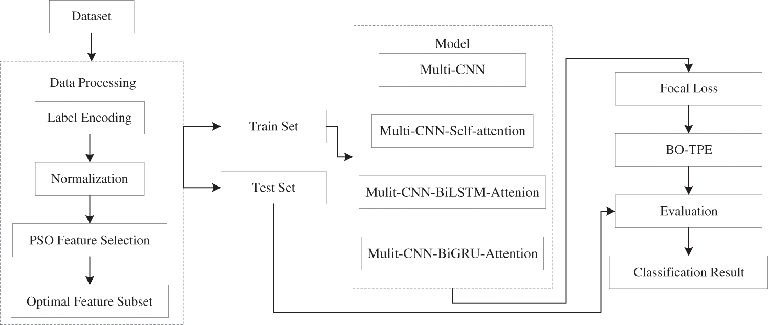
Figure 1: Architectures implemented in this research

3.1 Feature Selection

3.1.1 Particle Swarm Optimization

Recently, metaheuristic algorithms have gained significant prominence in the field of feature selection due to their exceptional global search capabilities [27]. Commonly used metaheuristic algorithms include Genetic-Algorithm (GA), Particle Swarm Optimization (PSO) [28], Whale Optimization Algorithm (WOA) [29], Grey Wolf Optimization (GWO) [30], Simulated Annealing (SA), and more. Among these, the PSO algorithm has garnered significant attention for its simplicity of implementation, minimal algorithm parameters, fast convergence, and strong optimization abilities. Kennedy et al. introduced the Particle Swarm Optimization (PSO) algorithm, which draws inspiration from the collective behavior of bird groups [28]. In the PSO algorithm, particles simulate bird predation behavior to find the optimal solution within a spatial range. In the search space, a group of particles is randomly generated, with each particle representing a candidate problem solution. By adjusting their speed, particles determine their direction and distance of movement. While moving to a new position, particles adjust their state based on their individual best position and the best position of the group, collectively flying toward the optimal position. Consequently, the entire population discovers the global optimal solution. Expressing an optimization problem in an N-dimensional space, each particle explores one dimension to locate the optimum solution. The update process for each particle is as follows:

Aim=(ai1m,ai2m,⋯,aiNm)(1)

Vim=(νi1m,νi2m,⋅⋅⋅,νiNm)(2)

vijm+1=kvijm+h1s1(pbestijm−aijm)+h2s2(qbestjm−aijm)(3)

aijm+1=aijm+vijm+1,j=1,2,…,N(4)

Here, h1 and h2 are acceleration coefficients, typically used to adjust the convergence speed of the particle swarm. s1 and s2 are random numbers ranging between 0 and 1, while k represents the inertia weight, used for balancing global and local search. m denotes the m-th iteration of the algorithm, pbestijm represents the best position recorded by the i-th particle up to the m-th movement, and qbestjm represents the best position recorded by the historical movements of the group particles.

Normally, the standard PSO algorithm is employed to solve optimization problems with continuous variables. In contrast, Kennedy and Eberhart proposed a binary PSO for solving discrete problems [31]. When applied to a binary feature selection problem, ‘1’ indicates the selection of a feature, while ‘0’ signifies the exclusion of a feature. The sigmoid function is utilized to transform the update formula:

ai,jm={1,rand≤sigmoid(νijm)0,1(5)

sigmoid(νijm)=11+e−νijm(6)

where rand represents a random number drawn from a uniform distribution between 0 and 1. Fig. 2 outlines the basic flowchart of the particle swarm optimization algorithm.

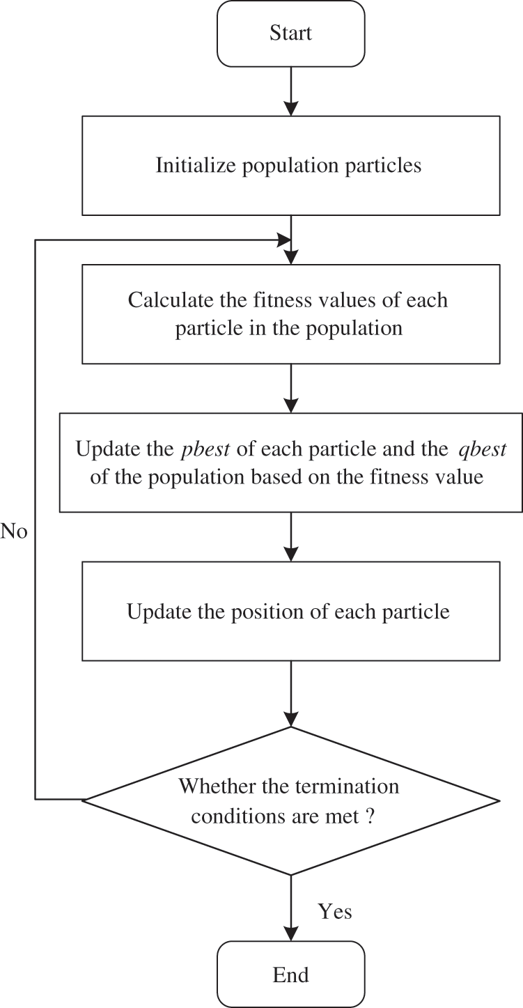
Figure 2: The PSO algorithm flow chart

3.2 Network Construction

Fig. 3 illustrates the Conv1d components of the four proposed models, while Fig. 4 provides an overview of the architecture of these models. The Multi-Conv1d model is a neural network that utilizes multi-scale one-dimensional convolutions. Each layer of the network consists of three convolution kernels of different sizes. Conv1d is well-suited for sequence processing as it slides convolution kernels of varying sizes over the input sequence, allowing it to capture features at different scales, ranging from local details to global patterns. Smaller kernels are effective at capturing local details, while larger kernels can identify longer dependencies. Pooling operations are then applied to reduce the dimensionality of the data, followed by a fully connected layer for classification purposes.

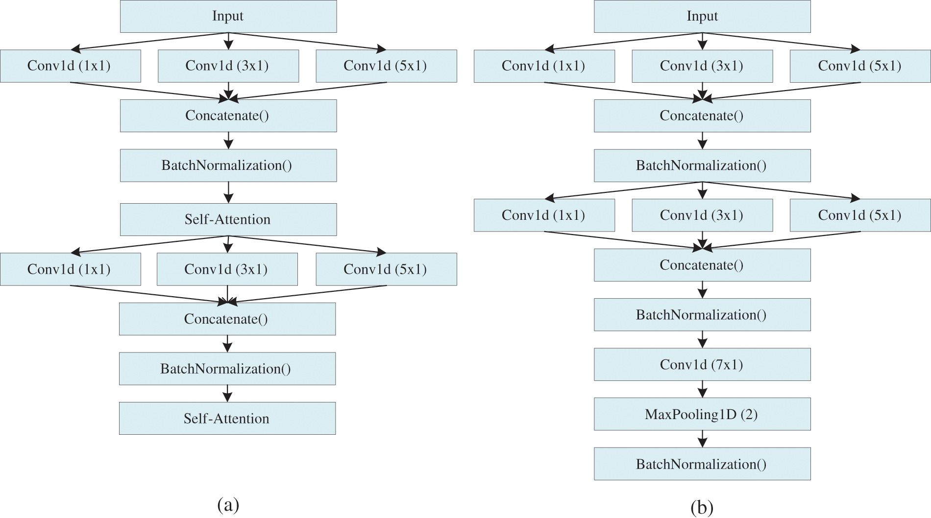
Figure 3: (a) Multi-Conv1d-Self-Attention-Head (b) Multi-Conv1d-Head

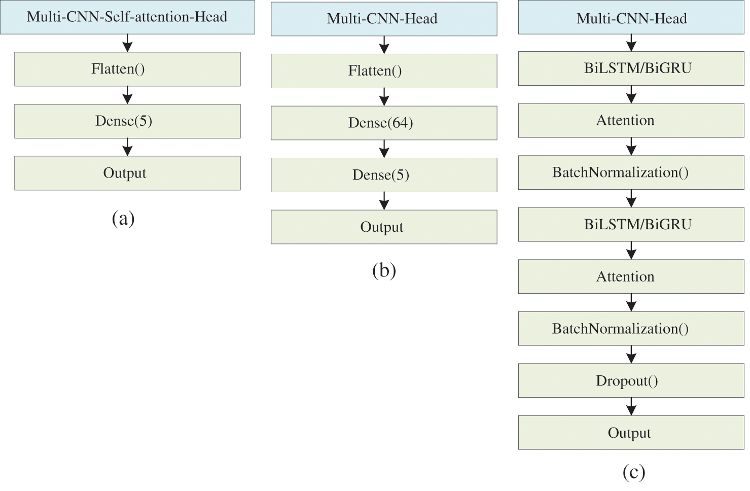
Figure 4: (a) Multi-Conv1d-Self-Attention (b) Multi-Conv1d (c) Multi-Conv1d-BiLSTM/BiGRU-Attention

The Multi-Conv1d-BiLSTM-Attention model incorporates Multi-Conv1d, BiLSTM, and Attention components. After preprocessing the data, it is inputted into the model. The convolution operation extracts local spatial features using a sliding window and reduces the model’s parameter count through weight sharing. The utilization of multiple convolution kernels enables the detection of local features at different scales, thereby improving model generalization. The introduction of the BatchNormalization layer ensures that the input distribution of each layer remains consistent during model training. This addresses the issue of difficult network training, accelerates model convergence, and helps prevent overfitting. Considering that network traffic follows a time series pattern, the BiLSTM component is capable of learning bidirectional time dependencies, facilitating effective processing of time series data and the extraction of time series features from network traffic. The attention mechanism is employed to guide the model’s focus towards important traffic features, ultimately improving model performance. The resulting output is the model’s prediction. The Multi-Conv1d-BiGRU-Attention model operates on a similar principle to the Multi-Conv1d-BiLSTM-Attention model, but with BiGRU containing fewer parameters than BiLSTM.

The Multi-Conv1d-Self-attention model is a neural network that combines multi-scale Conv1d and Self-attention. The self-attention mechanism provides a distinct advantage by computing the correlation between each element in the sequence and others, allowing for the identification of important features. By placing an attention layer after each multi-scale one-dimensional convolutional layer, the model can benefit from both multi-scale Conv1d and attention mechanisms, enabling the simultaneous extraction of spatiotemporal features from network traffic.

3.2.1 BiLSTM

RNN is effective in processing sequence data, but it faces issues of gradient disappearance and gradient explosion when training on long sequences. To address these problems, a neural network model called LSTM [32] has been developed as an improvement on RNN. LSTM units consist of an input gate, a forget gate, and an output gate, as shown in Fig. 5. They update parameters as follows:

ft=σ(Wfxt+Wfht−1+bf)(7)

it=σ(Wixt+Wiht−1+bi)(8)

ot=σ(Woxt+Woht−1+bo)(9)

c~t=tanh(Wcxt+Wcht−1+bc)(10)

ct=ft∗ct−1+it∗c~t−1(11)

ht=ot∗tanh(ct)(12)

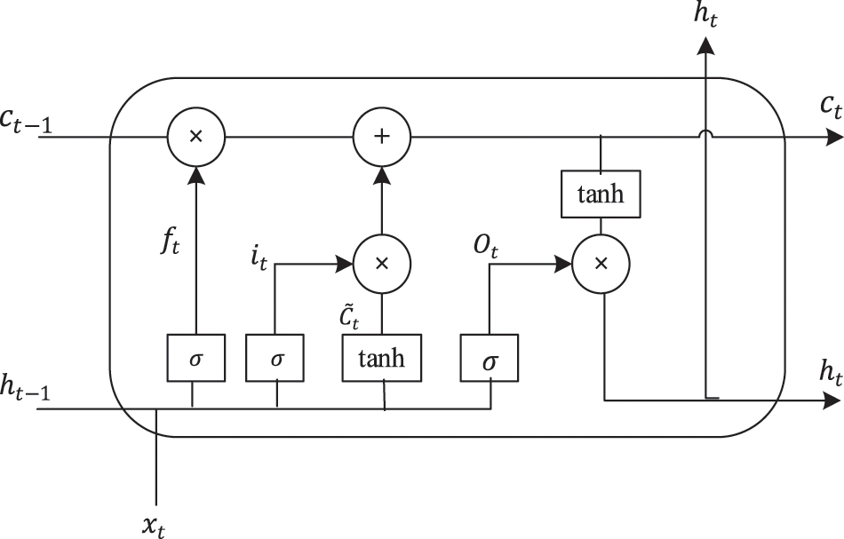
Figure 5: Structure diagram of LSTM

Here, σ represents the sigmoid function, Wf, Wi, Wo and Wc represent the corresponding weight matrices, and bf, bi, bo and bc represent the corresponding bias terms.

Bidirectional LSTM (BiLSTM) combines two LSTM networks, one for forward propagation and one for backward propagation. The outputs of these networks are then concatenated to form the output of BiLSTM:

ht→=C(Wt→,ht−1→,ct−1)(13)

h←t=C(Wt,h←t−1,ct−1)(14)

ht=[h→t,h←t](15)

Here, C represents the hidden layer of LSTM, and ht represents the output of BiLSTM.

3.2.2 BiGRU

The Gated Recurrent Unit (GRU) neural network [33] is a variant of the Recurrent Neural Network (RNN) and a simplified version of LSTM. It addresses the long-term memory and gradient problems in backpropagation [34]. GRU combines the input gate and forget gate of LSTM into an update gate, while maintaining the effectiveness of LSTM. The structure is simpler, resulting in faster model convergence. The structure of GRU is shown in Fig. 6. Parameters in GRU are updated as follows:

rt=σ(Wr∗[ht−1,xt])(16)

zt=σ(Wz∗[ht−1,xt])(17)

h~t=tanh(Wh~∗[rt∗ht−1,xt])(18)

ht=(1−zt)∗ht−1+zt∗h~t(19)

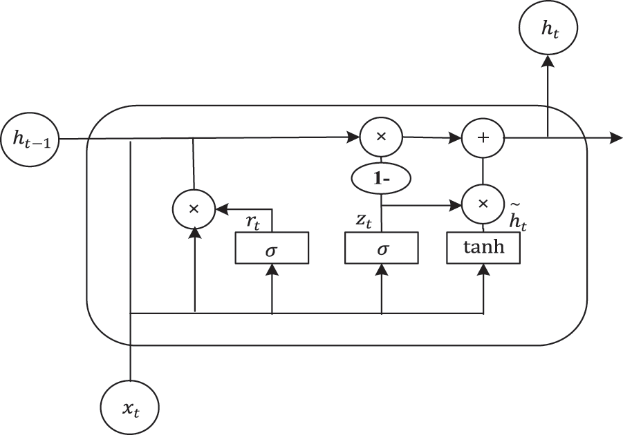
Figure 6: Structural diagram of GRU

Here, σ represents the sigmoid activation function, tanh represents the hyperbolic tangent activation function, rt and zt represent the reset gate and update gate at time t, respectively. Wr, Wz, and Wh~ represent the weight matrices of the GRU. ht represents the candidate hidden state at time t, ht represents the hidden state at time t, and ht−1 represents the hidden state at time (t-1). Fig. 6 shows the structural diagram of GRU.

The traditional GRU only utilizes the previous information of the sequence data. However, by using BiGRU, we can consider both the past and future states of the time series data when predicting the current situation. The basic unit of the Bidirectional Gated Recurrent Unit (BiGRU) model consists of a forward-propagating GRU unit and a backward-propagating GRU unit. BiGRU is structurally equivalent to the combination of positive and negative GRUs, and the result is jointly determined by these two GRUs. Fig. 7 shows the structure of BiGRU.

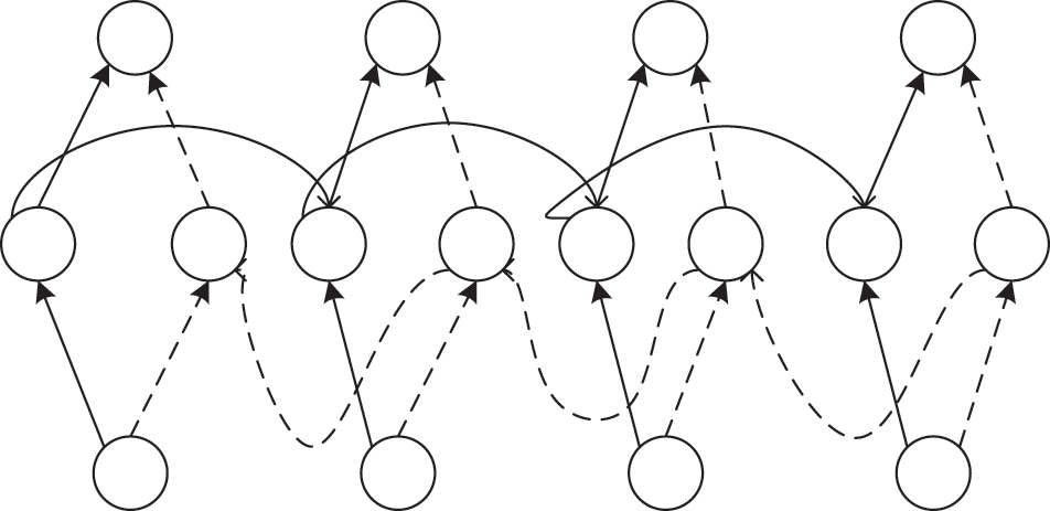
Figure 7: Structure diagram of BiGRU

ht→=GRU(xt,ht−1→)(20)

h←t=GRU(xt,h←t−1)(21)

ht=wtht→+vtht←+bt(22)

Among them, GRU(xt,ht−1→) represents the forward propagation of the GRU unit at time t, and GRU(xt,h←t−1) represents the backward propagation at time t. The GRU unit. wt and vt respectively represent the weights of the forward hidden layer transition ht→ and the backward hidden layer transition h←t corresponding to BiGRU at time t, and bt represents the bias at time t.

3.2.3 Attention

In recent years, the attention mechanism has been widely used in machine translation [35]. It is designed to allow the model to focus on important information rather than all information, effectively improving model performance [36]. Traditionally, machine translation encodes the entire input sentence into a fixed-length vector, and then decodes the translation using an encoder-decoder method. In [37], an attention mechanism was proposed, which allows the model to focus only on the relevant information and generate the next target without encoding the entire source sentence into a fixed-length vector. This improves the translation system’s performance when dealing with long sentences and avoids the need to pay attention to the entire input information. The attention mechanism establishes connections between the context vector and the entire source input, and the weights of these connections enable the model to pay more attention to important parts of the input. Multiple attentions are represented by calculating weights α(t,1), α(t,2),...,α(t,t). The context vector Ci of the output yi is computed as a weighted sum of these annotations hi:

Ci=∑j=1Tx⁡αijhj(23)

The weight αij of each annotation hj is computed by the softmax function:

αij=exp⁡(eij)∑k=1Tx⁡exp(eik)(24)

where

eij=a(si−1,hj)(25)

The function a(si−1,hj) describes the matching ability between the input around position j and the output at position i. The attention mechanism is introduced to give different attention to the information output by the hidden layer of GRU.

3.2.4 Self-Attention

The Self-Attention mechanism [36] can be used to extract the temporal characteristics of network traffic, and its main formula is:

Attention(Q,K,V)=softmax(QKTdkV)(26)

where dk represents the scaling factor.

3.2.5 Batch Normalization

The training process of deep neural networks is complex. The distribution of each batch of training data varies, and the network needs to adapt to different distributions in each iteration, which can slow down the convergence of the model. Batch Normalization [38] addresses these issues. It normalizes the data of the upper layer, bringing it into a unified interval and ensuring consistency in the input data distribution. It speeds up the convergence speed of model training, stabilizes the training process, and improves model accuracy. ℬ={x1…m} represents m activation values in the mini-batch, and γ and β are the parameters to be learned. First, calculate the mean and variance of ℬ:

μℬ←1m∑i=1m⁡xi(27)

σℬ2←1m∑i=1m⁡(xi−μℬ)2(28)

Second, normalize each activation value:

x^i←xi−μℬσℬ2+ϵ(29)

Finally, process each activation value with γ and β:

yi←γx^i+β(30)

3.3 Focal Loss

Focal loss is a known technique used to address category imbalance in machine learning, particularly in the context of deep learning models. In classification problems, the commonly used loss function is cross-entropy loss, which treats all categories equally. However, this approach may neglect minority class instances and bias the model towards the majority class.

In the field of intrusion detection, imbalanced datasets are prevalent, which can significantly impact classification results. Focal loss is an improvement over cross-entropy loss that introduces two adjustment factors, α and γ, to address this issue. These factors allow the model to focus on learning the minority class by adjusting the sample weights and difficulty.

The cross-entropy loss function is extensively used in deep learning classification. For binary classification, the binary cross-entropy loss can be defined as:

L(y,y^)=−(ylog(y^)+(1−y)log(1−y^))(31)

Here, y represents the true label and y^ represents the predicted value. This formulation can be extended to multi-classification, where the multi-class cross-entropy loss function is defined as:

L=1N∑i⁡Li=−1N∑i⁡∑c=1M⁡yiclog(pic)(32)

In the above equation, M denotes the number of categories, pic represents the predicted probability that sample i belongs to category c, and yic is a binary indicator (0 or 1) that indicates whether the true category of sample i is c.

The simplified expression for binary classification cross-entropy loss is:

CE(p,y)={−log(p),ify=1−log(1−p),otherwise(33)

Here, y = +1 or y = −1 corresponds to positive and negative samples, respectively, and p represents the probability of positive samples. To simplify notation, pt is defined as:

pt={pify=11−potherwise,(34)

In 2017, Lin et al. [39] introduced the focal loss function, which has gained popularity in computer vision applications to address imbalanced dataset issues. In our approach, we employ the focal loss function to train the deep model, effectively mitigating the impact of sample imbalance during training. Focal loss is a modification of the standard cross-entropy loss. By reducing the weight assigned to easily classifiable samples, the model can pay greater attention to challenging samples during training. The focal loss function can be defined as:

Loss=−αt(1−pt)γlog(pt)(35)

Here, (1−pt)γ serves as a modulating factor that reduces the weight of easily classifiable samples, and αt represents a weight factor used to address class imbalance.

3.4 BO-TPE

Hyperparameter tuning can generally be classified into four types: traditional manual tuning, grid search, random search, and Bayesian search. Manual parameter tuning heavily relies on experience and can be time-consuming. Neither grid search nor random search effectively utilize the correlation between different hyperparameter combinations. Bayesian Optimization is an adaptive method for hyperparameter search that predicts the next combination likely to yield the greatest benefit based on the previously tested hyperparameter combinations. In this study, we employ the Bayesian Optimization-Tree Parzen Estimator (BO-TPE) [40] technique to tune the model’s hyperparameters. BO-TPE demonstrates excellent global search capability and avoids falling into local optima. Random search is used during the initial iteration, where samples are drawn from the response surface to establish the initial distribution {θi,yi}(i=1,2,…,Ninit), where θ and y respectively represent the hyperparameter set and the corresponding value on the response surface. Two density functions, Prog(θ) and Prob(θ), are created within BO-TPE as the generative model for variables [41]. Good samples are distinguished from bad samples based on a predefined threshold y', as follows:

p(θ∣y)={ Prog(θ)ify < y′Prob(θ)ify≥y′(36)

Next, the Expected Improvement (EI) is calculated for each step:

El(θ)=Prog(θ)Prob(θ)(37)

Finally, the best hyperparameter values are selected by maximizing EI. Fig. 8 illustrates the flow diagram of BO-TPE.

Figure 8: Flowchart of BO-TPE

When optimizing the hyperparameters of the neural network model using BO-TPE, the primary hyperparameters to be tuned typically include batch size, learning rate, and dropout rate. Batch size represents the number of training samples used in each iteration, learning rate indicates the step size at each iteration, and dropout rate represents the probability of randomly deactivating neurons within the neural network.

4  Experiments and Results

4.1 Hardware and Environment Setting

We conducted our experiments on desktops equipped with the Windows Server 2019 operating system, 128 GB of RAM, an Intel(R) Xeon(R) Silver 4214 processor, and an RTX 3090 graphics card. To verify the feasibility of the proposed model, we used the Keras 2.3.1 deep learning framework and programmed in Python 3.7. The detailed experimental parameter configuration is presented in Table 1.

4.2 Evalution Metrics

In this paper, we use accuracy rate, recall rate, precision, precision recall, and F1-score as evaluation indicators to measure the performance of the proposed model. These indicators are represented by true positives (TP), true negatives (TN), false positives (FP), and false negatives (FN).

Accuracy=TP+TNTP+TN+FP+FN(38)

Precision=TPTP+FP(39)

Recall=TPTP+FN(40)

F1−score=2∗precision∗recallprecision+recall(41)

The specific definitions of TP, FP, FN, and TN in the field of intrusion detection are as follows: TP refers to the classification of an actual attack category as an attack category. FP refers to the classification of an actual normal category as an attack category. FN refers to the classification of an actual attack category as a normal category. TN refers to the classification of an actual normal category as a normal category. The confusion matrix formed by TP, FP, FN, and TN is depicted in Table 2, which visualizes the performance of detection.

4.3 Dataset

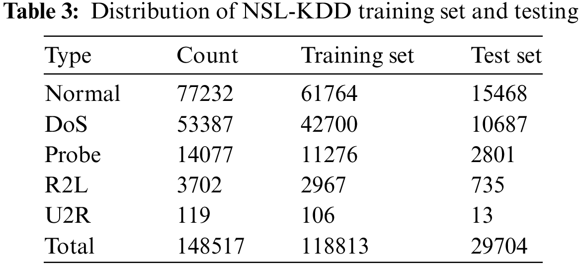
This article utilizes the NSL-KDD dataset as the experimental dataset. The data distribution and specific attack types are presented in Tables 3 and 4. The NSL-KDD [42] dataset is an enhanced version of KDDCup99, which eliminates duplicate data. It consists of a training set (KDDTrain+) with 125,973 samples and a test set (KDDTest+) with 22,544 samples. The NSL-KDD dataset has been provided by the University of New Brunswick. It encompasses four attack types: Denial of Service (DoS), Probing attacks (Probe), Remote to Local (R2L), and User to Root (U2R).

4.4 Data Preprocessing

Before inputting data into the model, the original dataset needs to undergo appropriate preprocessing. Data processing can be divided into four steps: label encoding, data normalization, and feature selection.

4.4.1 Label Encoding

The ‘protocol_type’, ‘service’, and ‘flag’ in NSL-KDD are character-type data. To convert them into numerical types, we use LabelEncoder for encoding.

4.4.2 Data Normalization

Once all features are converted into numerical values, the datasets need to be normalized. In this paper, we employ the Min-Max regularization method to scale the data between [0,1]. This helps reduce the adverse effects caused by singular sample data.

x′=x−xminxmax−xmin(42)

4.4.3 Feature Selection

To enhance the model’s generalization ability and prediction performance, we perform feature selection on the NSL-KDD dataset to remove redundant features and reduce computational overhead. For the PSO algorithm, the total population size is set to 50, and the number of iterations is set to 20. Both h1 and h2 are configured as 2, and k is set to 0.9. The PSO algorithm is utilized for this purpose, resulting in the selection of the 28 best features, as shown in Table 5.

4.5 Hyperparameter Optimization

During the experiment, we adopt the BO-TPE technique to adjust the model parameters. The parameter settings used in the search process are presented in Table 6. Parameters such as batch size, learning rate, and dropout rate are optimized to determine their optimal values.

4.6 Experimental Performance Evaluation

During the experiment, we divided the NSL-KDD dataset into a training set and a test set with proportions of 80% and 20%, respectively. The hyperparameters of the model were optimized using the BO-TPE method. In the field of intrusion detection, two scenarios are typically used to evaluate model performance: binary classification and multi-classification.

4.6.1 Binary Classification

In the binary classification scenario, the network traffic is divided into normal traffic and attack traffic. We evaluated four models and obtained the following results, as shown in Fig. 9. The Multi-Conv1d-Self-Attention model achieved the lowest performance in the binary classification experiment, with all four metrics at 0.99835. The best performance in the two-classification experiment was achieved by the Multi-Conv1d-BiLSTM-Attention model, with accuracy, precision, recall, and F1-score of 0.999158, 0.999159, 0.999158 and 0.999158, respectively. The Multi-Conv1d-BiLSTM-Attention model outperformed the Multi-Conv1d-BiGRU-Attention model by approximately 0.0001 in all four metrics. The confusion matrices of the four models for binary classification are shown in Fig. 10, where (a), (b), (c), and (d) represent Multi-Conv1d, Multi-Conv1d-Self-Attention, Multi-Conv1d-BiGRU-Attention, and Multi-Conv1d-BiLSTM-Attention, respectively.

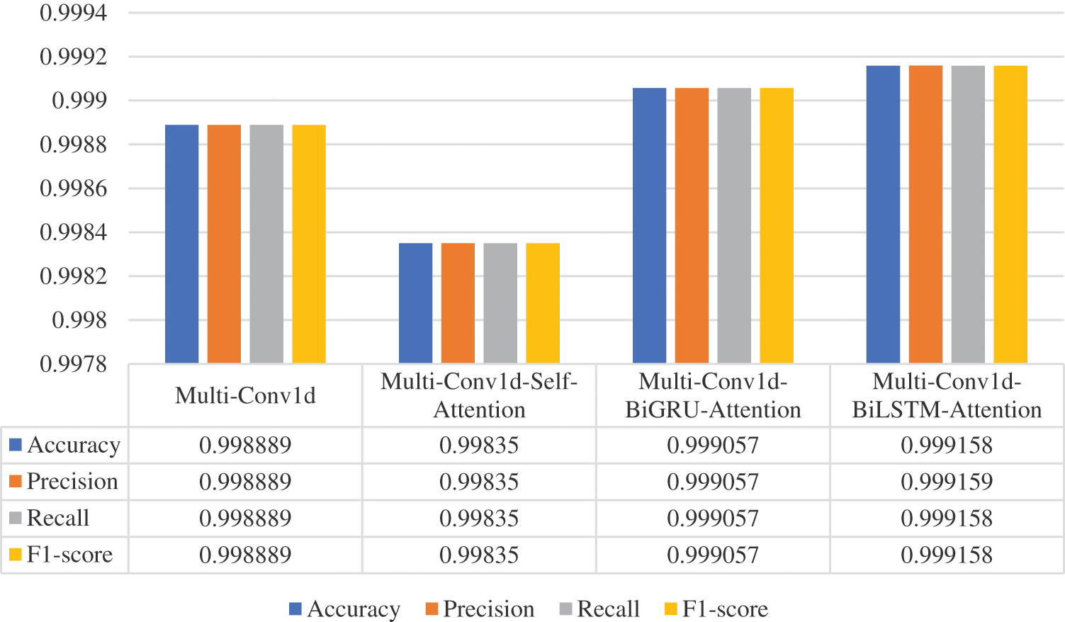
Figure 9: Binary classification results of the four proposed models on NSL-KDD

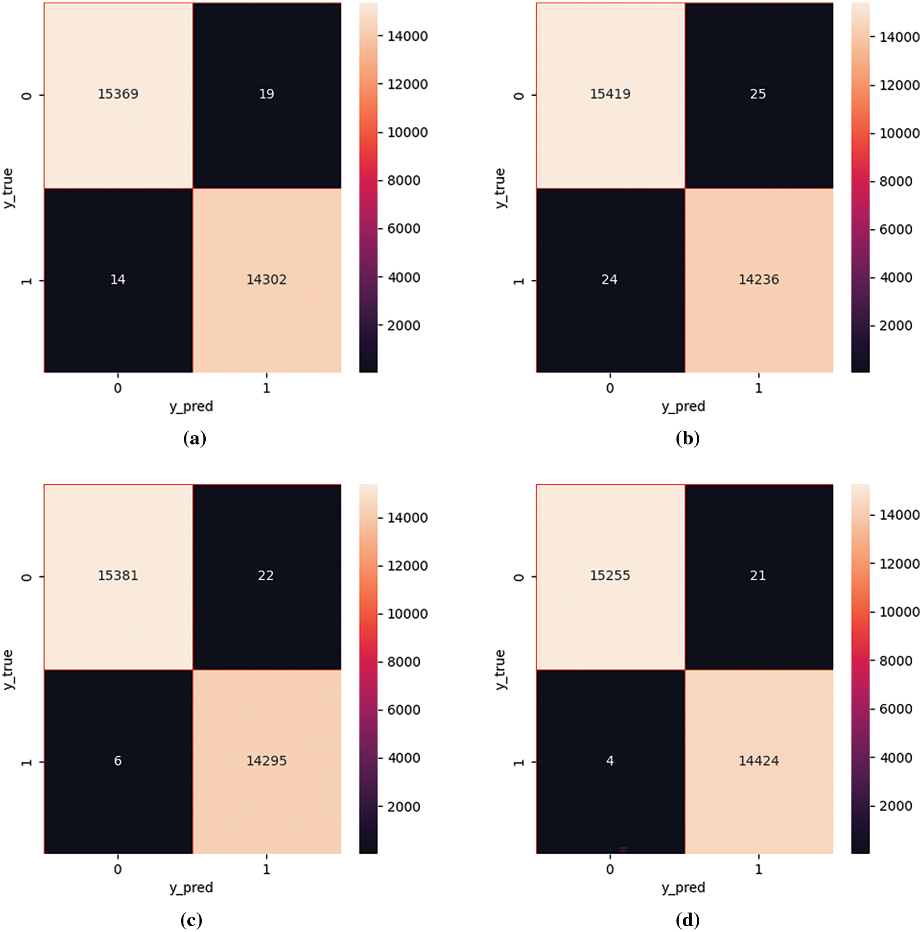
Figure 10: Binary classification confusion matrix diagram

4.6.2 Multi-Class Classification

In the multi-classification scenario, we classified the network traffic into multiple attack types along with the normal traffic. The experimental results and model parameters for the four models are shown in Figs. 11 and 12, respectively. It can be observed from the table that all four proposed models achieved a high accuracy of above 0.99, indicating their effectiveness in extracting features from the data and accurately predicting the categories. Additionally, the similar structures of the models resulted in very close values for each metric.

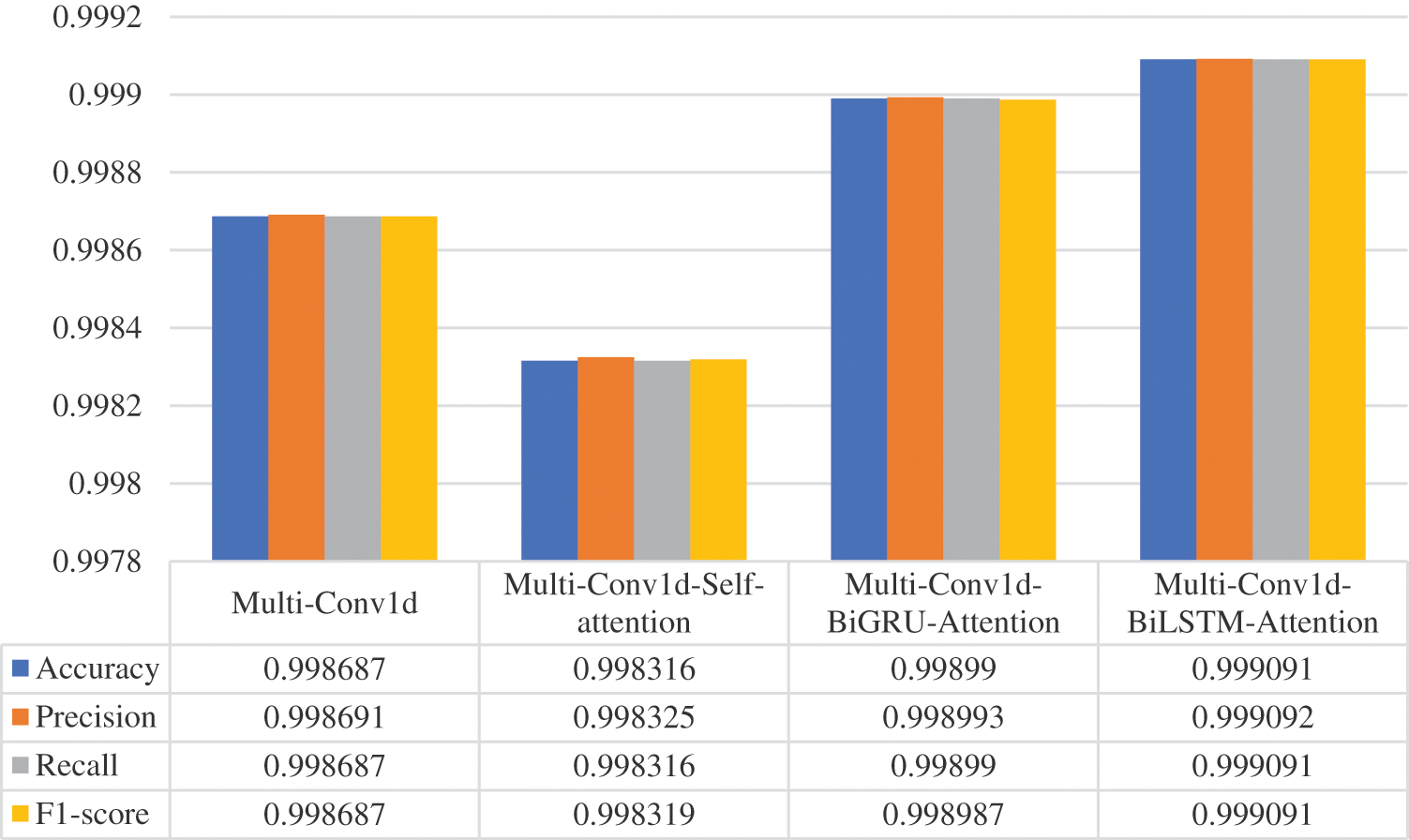
Figure 11: Results of multi-classification of the proposed four models on NSL-KDD

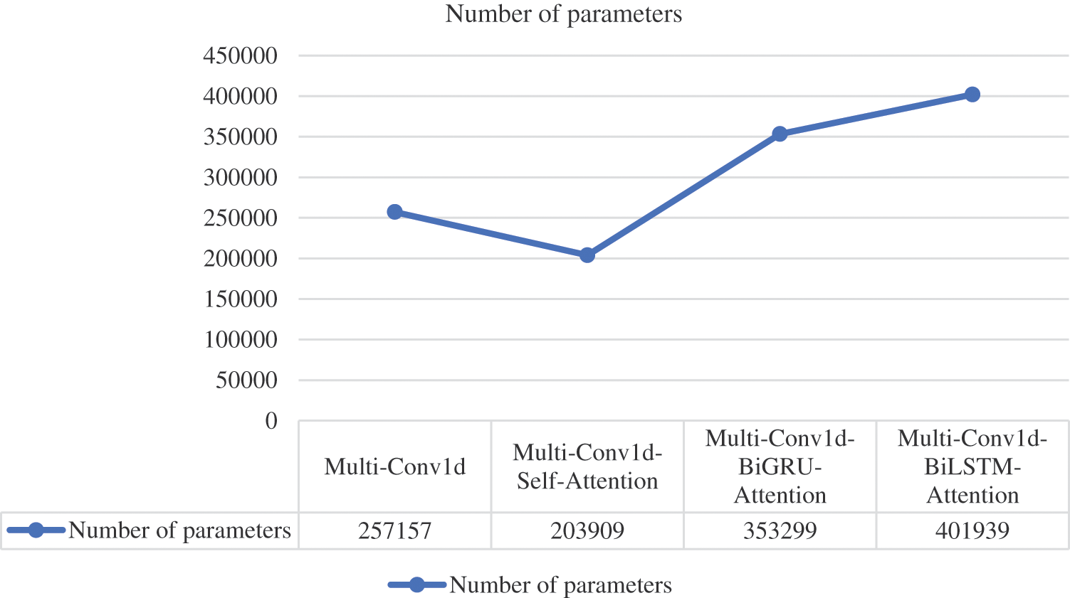
Figure 12: Model parameter quantity

The Multi-Conv1d-BiLSTM-Attention model performed best in all four metrics, demonstrating the advantages of incorporating BiLSTM and Attention mechanisms. The Multi-Conv1d model extracted spatial and local features at different scales, while BiLSTM captured the temporal relationships in the network traffic data through forward and backward modeling. The attention mechanism enabled the model to focus on important features. By combining these three components, the model effectively extracted spatiotemporal features and maximized classification performance. The Multi-Conv1d-BiGRU-Attention model ranked second, potentially due to the simpler structure of BiGRU compared to BiLSTM, which resulted in slightly weaker handling of long dependencies. The performance of Multi-Conv1d was slightly lower than that of Multi-Conv1d-BiLSTM-Attention and Multi-Conv1d-BiGRU-Attention since timing features were not extracted. The Multi-Conv1d-Self-Attention model, being relatively simple and having the fewest parameters, exhibited the worst performance. The number of parameters for the Multi-Conv1d-BiLSTM-Attention model was the highest at 401,939, while the Multi-Conv1d-Self-Attention model had the lowest at 203,909. Combining Figs. 11 and 12, we observed a direct proportional relationship between the number of model parameters and model performance. Model parameters also had an impact on the performance to some extent, with models having a larger number of parameters exhibiting stronger learning ability and better feature extraction.

In both the Multi-Conv1d-BiLSTM-Attention and Multi-Conv1d-BiGRU-Attention architectures, an Attention mechanism is employed. The Multi-Conv1d-BiLSTM and Multi-Conv1d-BiGRU structures often struggle to fully utilize the spatiotemporal information in the input, potentially leading to information loss or confusion. However, the introduction of the Attention mechanism addresses this issue. The Attention mechanism enables the model to automatically learn the crucial segments within the input sequence, enhancing the model’s focus on these segments. During each step of the model’s computation, the Attention mechanism assesses the importance of different segments within the input sequence and assigns corresponding weights to each of them. These weights express the contribution of different segments in the input sequence to the current computation. By utilizing these attention weights, the model can concentrate more on input segments with higher weights during each computation step, thereby extracting more valuable features. In the context of intrusion detection, the Attention mechanism can assist the model in better capturing important features and anomalous patterns within network traffic data.

The confusion matrices for the two classifications of the four models are shown in Fig. 13, where (a), (b), (c), and (d) represent Multi-Conv1d, Multi-Conv1d-Self-Attention, Multi-Conv1d-BiGRU-Attention, and Multi-Conv1d-BiLSTM-Attention, respectively.

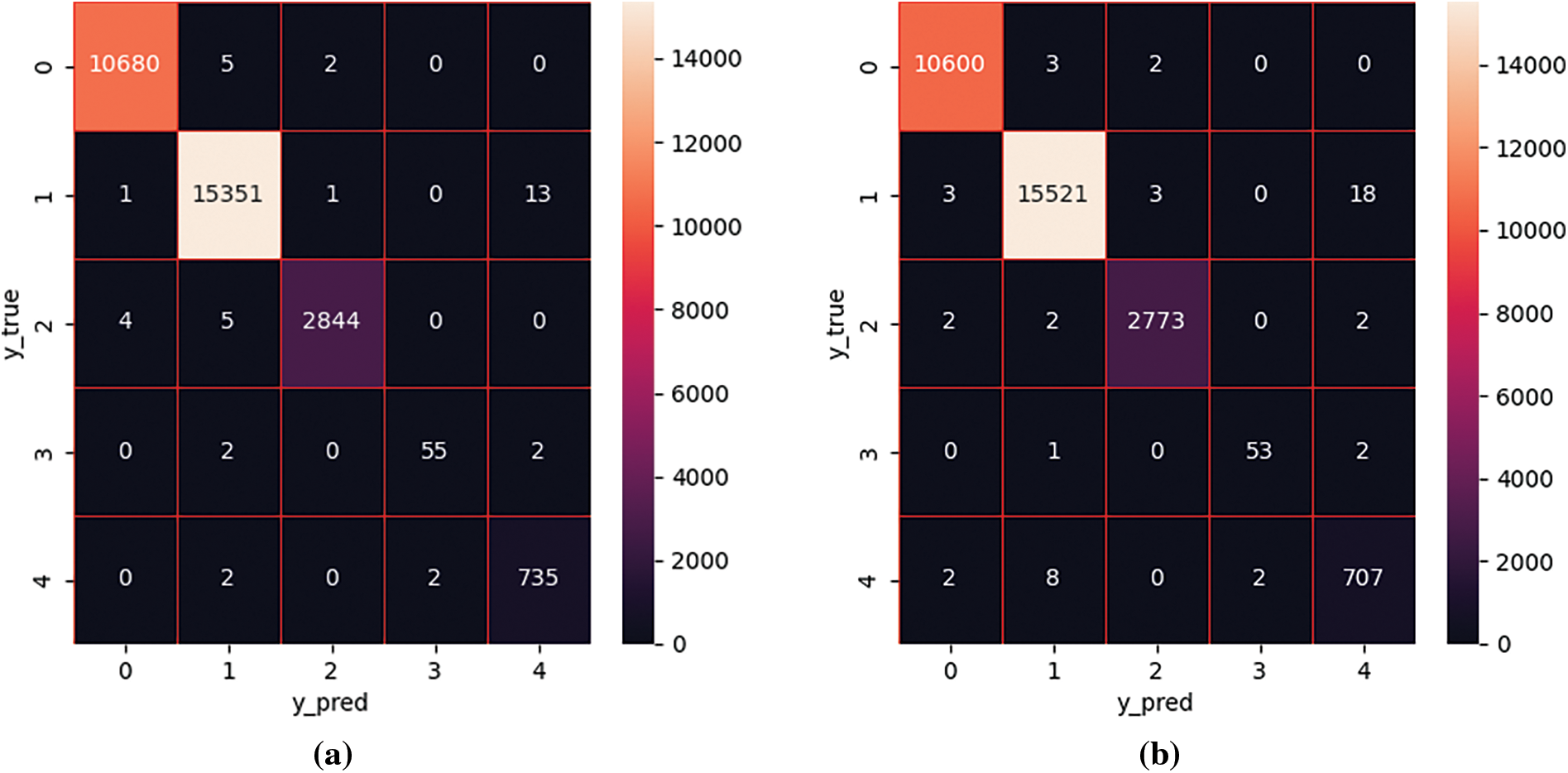
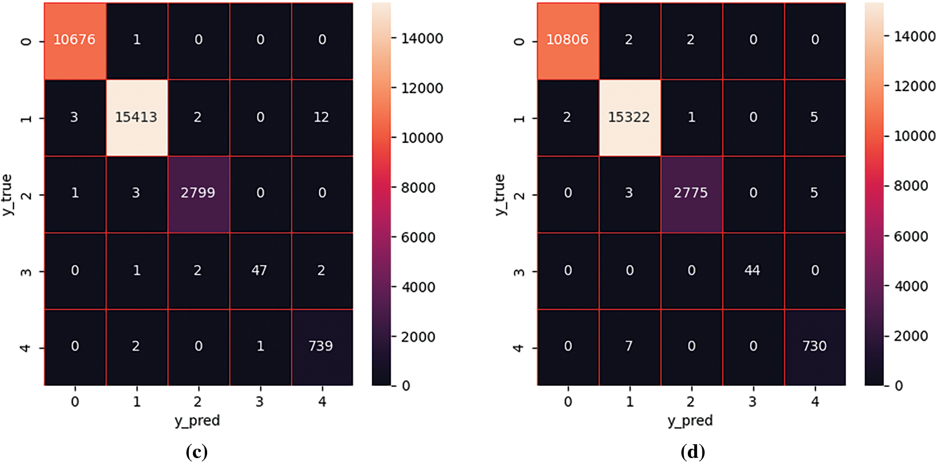
Figure 13: Multi-class confusion matrix diagram

Figs. 14–16 display the Precision, Recall, and F1-score achieved by the four models when classifying specific attack types in the dataset. The table highlights that Normal, DoS, and Probe have higher values for all three indicators, whereas U2R and R2L have lower values. Since Normal, DoS, and Probe have numerous variations, the models can effectively learn the characteristic representation of the data and perform accurate detection. Conversely, U2R and R2L have limited types, resulting in the models struggling to fully learn the feature representation and thus lower values are observed.

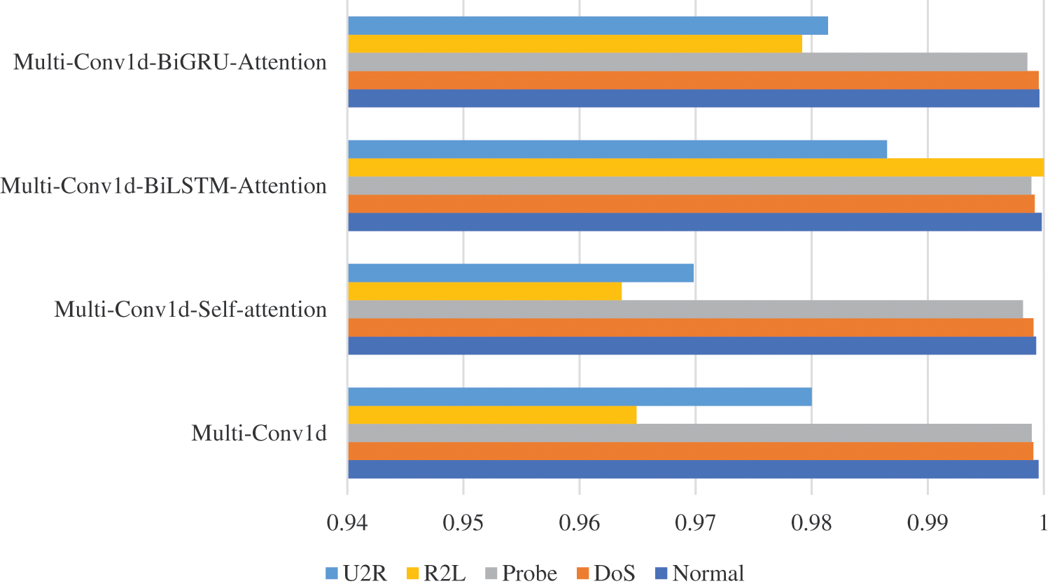
Figure 14: Precision of attack types

Figure 15: Recall of attack types

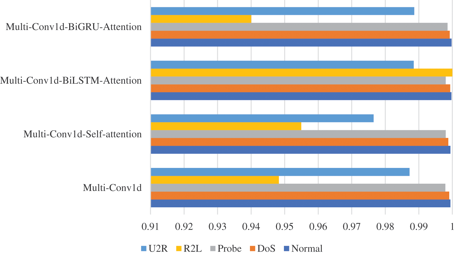
Figure 16: F1-score of attack types

4.6.3 Comparison with Other Methods

To establish a comparison with traditional machine learning methods, we evaluated NB, AdaBoost, LogisticRegression, and LightGBM. Fig. 17 demonstrates that LightGBM performs the best among these methods, with an accuracy of 0.979531. However, our proposed method outperforms all the traditional machine learning methods, achieving an accuracy of 0.999091. To further validate the performance of our proposed model, we compared it with other advanced methods, and the experimental results are presented in Table 7. Across all four metrics, our proposed model surpasses the other methods.

Figure 17: The comparison of the proposed model with existing machine learning methods

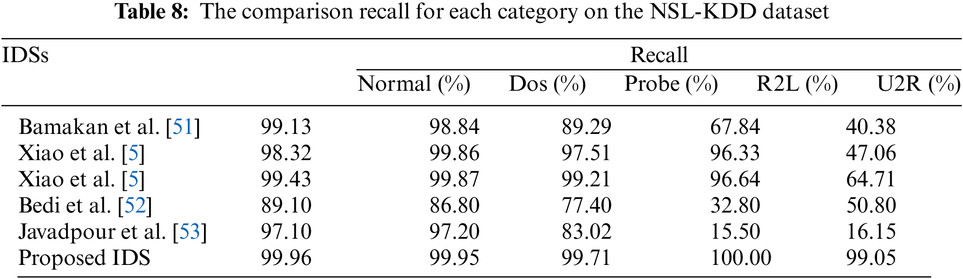
Additionally, we compared the per-category recall of our proposed IDS with other IDSs on the NSL-KDD dataset. Table 8 illustrates that our proposed IDS exhibits higher recall rates for each category, particularly for R2L and U2R, when compared to other IDSs.

Finally, one of our models was selected for experiments on the U2R category within the NSL-KDD dataset, utilizing two distinct loss functions: cross-entropy loss and focal loss. We proceeded to compare the performance of these two loss functions in the context of multi-class classification tasks, considering metrics such as Precision, Recall, and F1-score. The results are summarized in Table 9. From the data in the table, it is evident that the Recall for the U2R category improved significantly, rising from 0.916666 to a perfect 1.0. Moreover, Precision and F1-score also exhibited notable enhancements. During training with the cross-entropy loss function, the model had a tendency to accurately predict majority class samples while neglecting minority class samples. However, focal loss is a modification of the standard cross-entropy loss function that reduces the weight of easily classified samples. This modification encourages the model to focus more on challenging-to-classify samples during training.

5  Conclusion

In this paper, we present an intrusion detection method based on a deep neural network model. We utilize the NSL-KDD dataset, which comprises five different network traffic types. Four proposed models, namely Multi-Conv1d, Multi-Conv1d-Self-Attention, Multi-Conv1d-BiLSTM-Attention, and Multi-Conv1d-BiGRU-Attention, are employed for validation. Using a particle swarm optimization algorithm, we select the most important 28 features from a pool of 42. Among these four models, Multi-Conv1d-BiLSTM-Attention, through the combination of multi-scale Conv1d, BiLSTM, and Attention mechanisms, effectively extracts spatiotemporal features from network traffic data. We incorporate a Batch Normalization (BN) layer into the model to accelerate convergence and prevent overfitting, ultimately performing classification using a softmax function. We address the issues of data imbalance and model hyperparameter optimization using the Universal Focal Loss and Bayesian Optimization with Tree-structured Parzen Estimator (BO-TPE). The results in binary and multi-class classification show the highest accuracy, with values of 0.999158 and 0.999091, respectively. However, it is worth noting that the model has the highest parameter count, totaling 401,939. This implies that utilizing this model necessitates more significant computational resources. Although Multi-Conv1d-Self-Attention exhibits the poorest performance among the four models, it has the lowest parameter count, making it more suitable for operation in resource-constrained environments. In practical applications, the choice of the most suitable model should be based on resource constraints and performance requirements. Nevertheless, this also suggests that in the future, there is a need to explore model architectures with higher performance and lower resource consumption to enhance the availability of intrusion detection methods.

Acknowledgement: Not applicable.

Funding Statement: The authors received no specific funding for this study.

Author Contributions: The authors confirm contribution to the paper as follows: study conception and design: Bayi Xu, Lei Sun; data collection: Bayi Xu, Xiuqing Mao, Chengwei Liu, Zhiyi Ding; analysis and interpretation of results: Bayi Xu; draft manuscript preparation: Bayi Xu. All authors reviewed the results and approved the final version of the manuscript.

Availability of Data and Materials: Data will be made available on request.

Conflicts of Interest: The authors declare that they have no conflicts of interest to report regarding the present study.

References

1. L. Mohammadpour, T. C. Ling, C. S. Liew, and A. Aryanfar, “A survey of CNN-based network intrusion detection,” Appl. Sci., vol. 12, pp. 8162, 2022. [Google Scholar]

2. F. E. Laghrissi, S. Douzi, K. Douzi, and B. Hssina, “IDS-attention: An efficient algorithm for intrusion detection systems using attention mechanism,” J. Big Data, vol. 8, pp. 149, 2021. [Google Scholar]

3. V. Kumar, J. Srivastava, and A. Lazarevic, Managing Cyber Threats: Issues, Approaches, and Challenges. New York, USA: Springer Science+ Business Media, 2005. [Google Scholar]

4. Y. Yin et al., “IGRF-RFE: A hybrid feature selection method for MLP-based network intrusion detection on UNSW-NB15 dataset,” J. Big Data, vol. 10, no. 1, pp. 15, 2023. [Google Scholar]

5. Y. Xiao and X. Xiao, “An intrusion detection system based on a simplified residual network,” Information, vol. 10, no. 11, pp. 356, 2019. [Google Scholar]

6. D. E. Denning, “An intrusion-detection model,” IEEE Trans. Softw. Eng., vol. 13, no. 2, pp. 222–232, 1987. [Google Scholar]

7. A. Singh, J. Nagar, J. Amutha, and S. Sharma, “P2CA-GAM-ID: Coupling of probabilistic principal components analysis with generalised additive model to predict the k−barriers for intrusion detection,” Eng. Appl. Artif. Intell., vol. 126, pp. 107137, 2023. [Google Scholar]

8. G. P. Dubey and R. K. Bhujade, “Optimal feature selection for machine learning based intrusion detection system by exploiting attribute dependence,” Mater. Today: Proc., vol. 47, pp. 6325–6331, 2021. [Google Scholar]

9. Z. Halim et al., “An effective genetic algorithm-based feature selection method for intrusion detection systems,” Comput Secur., vol. 110, pp. 102448, 2021. [Google Scholar]

10. G. Chandrashekar and F. Sahin, “A survey on feature selection methods,” Comput. Electr. Eng., vol. 40, no. 1, pp. 16–28, 2014. [Google Scholar]

11. M. S. Milosevic and V. M. Ciric, “Extreme minority class detection in imbalanced data for network intrusion,” Comput. Secur., vol. 123, pp. 102940, 2022. [Google Scholar]

12. K. Ren, S. Yuan, C. Zhang, Y. Shi, and Z. Q. Huang, “CANET: A hierarchical CNN-attention model for network intrusion detection,” Comput. Commun., vol. 205, pp. 170–181, 2023. [Google Scholar]

13. R. Vinayakumar et al., “Deep learning approach for intelligent intrusion detection system,” IEEE Access, vol. 7, pp. 41525–41550, 2019. [Google Scholar]

14. H. Wang, Z. Cao, and B. Hong, “A network intrusion detection system based on convolutional neural network,” J. Intell. Fuzzy Syst., vol. 38, no. 6, pp. 7623–7637, 2020. [Google Scholar]

15. A. El-Ghamry, A. Darwish, and A. E. Hassanien, “An optimized CNN-based intrusion detection system for reducing risks in smart farming,” Internet Things, vol. 22, pp. 100709, 2023. [Google Scholar]

16. A. A. Malibari et al., “A novel metaheuristics with deep learning enabled intrusion detection system for secured smart environment,” Sustain. Energ. Technol. Assess., vol. 52, pp. 102312, 2022. [Google Scholar]

17. V. Murali Mohan, R. M. Balajee, K. M. Hiren, B. R. Rajakumar, and D. Binu, “Hybrid machine learning approach based intrusion detection in cloud: A metaheuristic assisted model,” Multiagent Grid Syst., vol. 18, no. 1, pp. 21–43, 2022. [Google Scholar]

18. J. V. A. Sukumar, I. Pranav, M. M. Neetish, and J. Narayanan, “Network intrusion detection using improved genetic k-means algorithm,” in Proc. 2018 ICACCI, Bangalore, India, 2018, pp. 2441–2446. [Google Scholar]

19. S. M. Kasongo and Y. Sun, “Performance analysis of intrusion detection systems using a feature selection method on the UNSW-NB15 dataset,” J. Big Data, vol. 7, no. 1, pp. 105, 2020. [Google Scholar]

20. S. Ustebay, Z. Turgut, and M. A. Aydin, “Intrusion detection system with recursive feature elimination by using random forest and deep learning classifier,” in Proc. 2018 IBIGDELFT, Ankara, Turkey, 2018, pp. 71–76. [Google Scholar]

21. T. Wu et al., “Intrusion detection system combined enhanced random forest with SMOTE algorithm,” EURASIP J. Adv. Signal Process., vol. 2022, pp. 39, 2022. [Google Scholar]

22. J. Man and G. Sun, “A residual learning-based network intrusion detection system,” Secur. Commun. Netw., vol. 2021, pp. 5593435, 2021. [Google Scholar]

23. H. Ding, L. Chen, L. Dong, Z. Fu, and X. Cui, “Imbalanced data classification: A KNN and generative adversarial networks-based hybrid approach for intrusion detection,” Future Gen. Comput. Syst., vol. 131, pp. 240–254, 2022. [Google Scholar]

24. F. Laghrissi, S. Douzi, K. Douzi, and B. Hssina, “Intrusion detection systems using long short-term memory (LSTM),” J. Big Data, vol. 8, pp. 65, 2021. [Google Scholar]

25. S. M. Othman, F. M. Ba-Alwi, N. T. Alsohybe, and A. Y. Al-Hashida, “Intrusion detection model using machine learning algorithm on big data environment,” J. Big Data, vol. 5, no. 1, pp. 34, 2018. [Google Scholar]

26. D. Akgun, S. Hizal and U. Cavusoglu, “A new DDoS attacks intrusion detection model based on deep learning for cybersecurity,” Comput. Secur., vol. 118, pp. 102748, 2022. [Google Scholar]

27. X. Li and J. Ren, “MICQ-IPSO: An effective two-stage hybrid feature selection algorithm for high-dimensional data,” Neurocomputing, vol. 501, pp. 328–342, 2022. [Google Scholar]

28. J. Kennedy and R. Eberhart, “Particle swarm optimization,” in Proc. ICNN’95, Perth, WA, Australia, 1995, pp. 1942–1948. [Google Scholar]

29. M. Mafarja and S. Mirjalili, “Whale optimization approaches for wrapper feature selection,” Appl. Soft Comput., vol. 62, pp. 441–453, 2018. [Google Scholar]

30. S. Mirjalili, S. M. Mirjalili, and A. Lewis, “Grey wolf optimizer,” Adv. Eng. Softw., vol. 69, pp. 46–61, 2014. [Google Scholar]

31. J. Kennedy and R. C. Eberhart, “A discrete binary version of the particle swarm algorithm,” in IEEE Trans. Syst. Man Cybern., Orlando, FL, USA, 1997, pp. 4104–4108. [Google Scholar]

32. S. Hochreiter and J. Schmidhuber, “Long short-term memory,” Neural Comput., vol. 9, pp. 1735–1780, 1997. [Google Scholar] [PubMed]

33. J. Chung, C. Gulcehre, K. Cho, and Y. Bengio, “Empirical evaluation of gated recurrent neural networks on sequence modeling,” arXiv preprint arXiv:1412.3555, 2014. [Google Scholar]

34. J. R. Zhang, F. A. Liu, W. Z. Xu and H. Yu, “Feature fusion text classification model combining CNN and BiGRU with multi-attention mechanism,” Future Internet, vol. 11, pp. 237, 2019. [Google Scholar]

35. J. Chorowski, D. Bahdanau, D. Serdyuk, K. Cho, and Y. Bengio, “Attention-based models for speech recognition,” in NIPS 2015, Montreal, Quebec, Canada, 2015, pp. 577–585. [Google Scholar]

36. A. Vaswani et al., “Attention is all you need,” in NIPS 2017, Long Beach, CA, USA, 2017, pp. 6000–6010. [Google Scholar]

37. D. Bahdanau, K. Cho, and Y. Bengio, “Neural machine translation by jointly learning to align and translate,” arXiv preprint arXiv:1409.047, 2014. [Google Scholar]

38. S. Ioffe and C. Szegedy, “Batch normalization: Accelerating deep network training by reducing internal covariate shift,” in Proc. 32nd Int. Conf. on Mach. Learn., Lille, France, 2015, pp. 448–456. [Google Scholar]

39. K. M. He, G. Gkioxari, P. Dollar, and R. Girshick, “Mask R-CNN,” in Proc. 2017 ICCV, Venice, Italy, 2017, pp. 2980–2988. [Google Scholar]

40. J. Bergstra, R. Bardenet, Y. Bengio, and B. Kegl, “Algorithms for hyper-parameter optimization,” in Proc. 24th Int. Conf. Neural Inf. Process. Syst., Granada, Spain, 2011, pp. 2546–2554. [Google Scholar]

41. L. Yang and A. Shami, “On hyperparameter optimization of machine learning algorithms: Theory and practice,” Neurocomput., vol. 415, pp. 295–316, 2020. [Google Scholar]

42. M. Tavallaee, E. Bagheri, W. Lu, and A. A. Ghorbani, “A detailed analysis of the KDD CUP 99 data set,” in 2009 IEEE Symp. Comput. Intell. Secur. Defense Appl., 2009, pp. 1–6. [Google Scholar]

43. I. Benmessahel, X. Xie, and M. Chellal, “A new evolutionary neural networks based on intrusion detection systems using multiverse optimization,” Appl. Intell., vol. 48, pp. 2315–2327, 2018. [Google Scholar]

44. N. Kunhare, R. Tiwari, and J. Dhar, “Intrusion detection system using hybrid classifiers with meta-heuristic algorithms for the optimization and feature selection by genetic algorithm,” Comput. Electr. Eng., vol. 103, pp. 108383, 2022. [Google Scholar]

45. S. K. Gupta, M. Tripathi, and J. Grover, “Hybrid optimization and deep learning based intrusion detection system,” Comput. Electr. Eng., vol. 100, pp. 107876, 2022. [Google Scholar]

46. J. Gu and S. Lu, “An effective intrusion detection approach using SVM with naïve Bayes feature embedding,” Comput. Secur., vol. 103, pp. 102158, 2021. [Google Scholar]

47. J. Sinha and M. Manollas, “Efficient deep CNN-BiLSTM model for network intrusion detection,” in Proc 2020 3rd Int. Conf. Artif. Intell. Pattern Recogn., Xiamen, China, 2020, pp. 223–231. [Google Scholar]

48. A. Li and S. Yi, “Intelligent intrusion detection method of industrial Internet of things based on CNN-BiLSTM,” Secur. Commun. Netw., vol. 2022, pp. 5448647, 2022. [Google Scholar]

49. A. S. Dina, A. B. Siddique, and D. Manivannan, “A deep learning approach for intrusion detection in Internet of Things using focal loss function,” Internet of Things, vol. 22, pp. 100699, 2023. [Google Scholar]

50. B. Cao, C. Li, Y. Song, Y. Qin, and C. Chen, “Network intrusion detection model based on CNN and GRU,” Appl. Sci., vol. 12, no. 9, pp. 4184, 2022. [Google Scholar]

51. S. M. H. Bamakan, H. Wang, Y. Tian, and Y. Shi, “An effective intrusion detection framework based on MCLP/SVM optimized by time-varying chaos particle swarm optimization,” Neurocomputing, vol. 199, pp. 90–102, 2016. [Google Scholar]

52. P. Bedi, N. Gupta, and V. Jindal, “I-SiamIDS: An improved Siam-IDS for handling class imbalance in network-based intrusion detection systems,” Appl. Intell., vol. 51, pp. 1133–1151, 2021. [Google Scholar]

53. A. Javadpour, P. Pinto, F. Ja’fari, and W. Zhang, “DMAIDPS: A distributed multi-agent intrusion detection and prevention system for cloud IoT environments,” Cluster Comput., vol. 26, no. 1, pp. 367–384, 2023. [Google Scholar]