A Review of Computing with Spiking Neural Networks

1  Introduction

In the past decade, artificial neural networks (ANNs) have made great achievements in the field of machine learning, and their performance is a revolutionary breakthrough compared to the traditional machine learning methods based on expert systems. ANNs have been successfully applied in many fields, including medical diagnosis [1], network security detection [2], image processing [3], agricultural production [4], and so on. However, although existing ANNs are brain-inspired, they are mainly modeled by abstracting neural structures at the mathematical level and still lack biological plausibility in terms of structure, information transfer, learning rules, and so on. In addition, ANNs require a large amount of energy consumption during its computation, for example, the backbone network of the large language model, ChatGPT, contains 175 billion learnable parameters, and it’s estimated that the training process consumes about 190,000 kWh of energy [5]. In contrast, the power consumption of the human brain is only about 20 W [6]. To bridge the gap between artificial neural networks and biological neural networks, the concept of spiking neural networks (SNNs) is gradually developed. SNNs are known as the third generation of neural networks. Compared with ANNs, SNNs are more bionic to the biological brain. SNNs simulate the propagation of biological signals in neural networks in the form of spike sequences, which are sparse and event-driven. This makes SNNs more energy-efficient than ANNs which use continuous values to represent information. Spike sequences are discrete events in the time dimension, which means that SNNs can capture information in the time domain like biological neurons, not only in the spatial dimension. In addition, SNNs are constructed based on neuron models that have closer modeling of neural dynamics, which is to say SNNs fully simulate the biological neural network system in terms of network construction.

As an interdisciplinary field between neuroscience and artificial intelligence, there are two main research directions in the development of SNNs. One is in the field of neuroscience and brain science to understand the mechanism of brain action by simulating the computational model of the nervous system. The other is to develop and apply SNNs in the field of intelligent computing and machine learning, etc. Therefore, SNNs provide a powerful approach for the cross-fusion of artificial intelligence and neuroscience to establish true brain-like computing.

Currently, research related to SNNs is in a rapidly developing state. Earlier, some scholars have reviewed and summarized the research progress of SNNs. However, in the past several years, SNNs have continuously made new achievements in supervised learning algorithms, software and hardware platforms, etc., and have pushed the performance of SNNs to a new level. It is urgent to sort out the latest research directions and achievements of SNNs. There are also literature reviews such as reference [7] which focus more on introducing SNNs from the interdisciplinary perspective of biological neuroscience and computational science, emphasizing the interdisciplinary advantages of SNNs. Currently, there is still a lack of SNN review literature focusing on enhancing processing performance and improving the practicality of development and application, which is not conducive to beginners, and application researchers to obtain an efficient way to start with SNNs. Starting from this issue, this paper elaborates on SNNs along the complete usage process of SNNs including network construction, data processing, model training, development, and deployment. And this paper focuses on the development of SNNs in the field of intelligent computing and machine learning in recent years, to provide more comprehensive and practical guidance to promote the development of SNNs.

The rest of this paper is organized as follows. Section 2 describes the network structure of SNNs, including its neuron model, synapses, and network topology. Section 3 describes the dataset used by SNNs and the data process methods. Section 4 focuses on the learning algorithms of SNNs, and introduces the research results of the training algorithms of SNNs so far from the perspectives of unsupervised and supervised learning. Section 5 introduces the software programming framework and the specific hardware platform, which is important for improving the research efficiency and promoting the application of SNNs. Section 6 summarizes the work of this paper, sorts out the main problems to be solved in SNNs, and looks forward to the future development direction.

2  Network Components

In the network construction aspect of SNNs, this chapter presents the basic components of spiking neural networks, including the neuron model, the spiking neuron synapses, and the neural network topology. We will review the basic knowledge and research progress of SNNs network components from the perspective of SNN’s computing performance and practicability.

2.1 Neuron Model

The neuron model is the basic unit of the neural network. The input and output of traditional artificial neural network neurons are continuous real values. As shown in Fig. 1a, The neurons perform weighted sum operations on the input signal and then output the signal xOUT through a nonlinear activation function f. Compared to ANNs, the neurons in SNNs provide a more in-depth and detailed simulation of biological neuronal behavior. As shown in Fig. 1b, like biological neurons, spiking neurons are divided into three parts: dendrites, cell body, and axons. And neurons are connected by synapses. In SNNs, the behavior of spike neurons is mainly controlled by membrane potential V and activation threshold Vth. The spike signal received by the neuron dendrites changes the membrane potential of the neuron. When the membrane potential accumulated by the neuron reaches the activation threshold, the neuron fires a spike signal sOUT from the axon to the neuron at the next layer. It can be seen that the spiking neuron can better simulate the membrane potential change and charge-discharge mechanism of biological neurons, and this is completely different from the artificial neuron based on addition and multiplication operations and nonlinear activation functions.

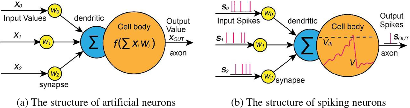
Figure 1: A comparison between artificial neuron and spike neuron

There are several specific neuron models for building SNNs. Among them, the integrate-and-fire (IF) model, leaky integrate-and-fire (LIF) model, and spike response model (SRM) are widely used in intelligent computing research due to their high computational efficiency.

2.1.1 Integrate-and-Fire Model and Leaky Integrate-and-Fire Model

The Integrated-and-fire model is one of the earliest neuron models, which was proposed in the early 20th century. Limited by the level of research at that time, the behavior of neurons was simply described as following [8]. Charging: the input spikes are integrated to the membrane potential. Firing: if the accumulation exceeds the set threshold, the output spike will be fired. Reset: After firing, the membrane potential resets to the resting state. The charging, firing, and reset behavior can be expressed as the following three equations:

I(t)=CMdVdtX(t)={1,if V≥Vth0,if V<Vth}V←Vrest, if V≥Vth(1)

where CM is the membrane capacitance, V is the membrane potential, Vth is the threshold potential, Vrest is the resting potential, I(t) represents the input current of the cell membrane, and X(t) denotes the output from the axon of the neuron.

The LIF model [9] adds a potential leakage mechanism to the IF model. Under the action of the potential leakage mechanism, when there is no new input stimulus, the membrane potential of the neuron will gradually return to the resting potential. This makes the LIF model closer to the operation mechanism of biological neurons than the IF model. At this time, the LIF model can be expressed as:

τMdVdt=Vrest−V+RMI(t)X(t)={1,if V≥Vth0,if V<Vth}V←Vrest if V≥Vth(2)

where τM=RMCM is the leakage time constant, RM denotes the impedance of the cell membrane. And the meanings of the remaining parameters are consistent with the IF model. In the above reset equation of IF and LIF model, the membrane potential is restored to the resting potential, and this type of reset now called hard reset. Correspondingly, there is another reset method called soft reset, which is proposed by Rueckauer et al. [10], i.e., after releasing the spike, the membrane potential is subtracted from the threshold voltage as shown in Eq. (3):

V←(V−Vth)ifV≥Vth.(3)

The soft reset approach can make the performance of IF neuron’s firing rate close to the ReLu function in ANNs [10], which is widely used in SNNs trained by the ANN converting method.

The IF and LIF models do not model the dynamic changes of ion channels in biological neurons, but only describe the key features of membrane potential such as accumulation, firing, and leakage (leakage is only in the LIF model). Therefore, they are computationally simple, with a low computational cost of only 5 floating point operations per second (FLOPS) per 1-ms simulation [11]. And they are easy to implement in large-scale network and hardware designs, and have the lowest power consumption. However, the IF and LIF models still have the disadvantage of insufficient biological plausibility and are not suitable for simulations that require high biological realism.

For intelligent computing and machine learning scenarios, some scholars have also improved the IF or LIF neuron structure to improve the practicability of SNNs. Besides the soft reset approach mentioned earlier, another route is to make the hyperparameters in the neurons trainable, such as the Parametric-LIF (PLIF) model proposed by Fang et al. [12], which has a learnable time constant τM to enhance the learning effect of SNNs. There are also attempts to expand the representation range of neurons to the negative domain to enhance the network’s expression ability, such as in references [13–15]. These neurons usually achieve the expression of negative information such as negative threshold voltage and negative excitation. For the hardware implementation of LIF neurons, the Euler equation is usually used to convert the original differential equation into a difference equation. While Ye et al. [16] used optimization method of extended prediction correction (EPC) and proposed the EPC-LIF model, to provide higher stability and smaller transformation error compared to the direct use of Euler equations.

2.1.2 Spike Response Model

There is refractory period for a biological neuron in the short time after firing, that means the neuron does not respond to the input signal during this period. The Spike Response Model [17,18] adds the simulation of the refractory period to the LIF model. And the filters (kernel functions), rather than the differential equations in LIF model, are used to describe the effects and responses of external inputs or its own activation state on the membrane potential. The mathematical formulation is as follows:

V(t)=∑fη(t−t(f))+Vrest+∫0∞κ(s)I(t−s)ds(4)

where V(t) is the membrane potential, Vth is the threshold potential, Vrest is the resting potential, t(f) is the time when the f-th spike of a neuron is generated. η is called the kernel function of the refractory period, which describes both the effect of the spike at t(f) time on the action potential and the subsequent potential changes. κ is a linear filter describing the effect of the input current, I(t−s), at time (t−s) on the membrane potential.

SRM model is better than LIF model in biological plausibility, but its computational cost also increases, requiring 50 FLOPS per 1-ms simulation [19]. When implemented in a digital system, the calculation of SRM model is relatively complex. However, the equations of this model can be modeled with analog circuits because its postsynaptic potential function can be considered as the charging and discharging of an resistor-capacitance circuit [20]. In addition, because the SRM model uses explicit equations rather than differential equations to describe the activity of neurons, the output of neurons can be calculated directly after a given input. Thus, the behavior of neurons can be easily studied by analyzing the equation.

In addition to the above models, there are also models such as the Hodgkin Huxley (H-H) model [21] and Izhikevich model [22] that focus more on simulating the characteristics of biological neurons, but their computational efficiency is relatively low. The summary of these neuron models is shown in Table 1.

2.2 Synapses of Spiking Neurons

Synapses are the connecting nodes between neurons and are the basic storage elements that enable memory and learning in neural networks. As shown in Fig. 1b, spiking signals generated by a presynaptic neuron, si(i=0,1,2,…), are transmitted through the synapse to the dendrites of a postsynaptic neuron. For the postsynaptic neuron, the input signal is regulated by wi(i=0,1,2,…), the weight of the corresponding synapse, and finally converged into an input current I, which has an excitatory or inhibitory effect on the postsynaptic neuron to change its membrane potential. Therefore, the learning of a spiking neural network is a process of constantly adjusting the synaptic weights of neurons according to a specific training rule in order to achieve an optimal solution.

2.3 Network Topology

Multiple neurons are interconnected to form a hierarchical structure of spiking neural networks. Depending on the type of connections used, spiking neural networks have a variety of topology types. Like traditional artificial neural networks, the main topologies of SNNs are feedforward neural networks, recurrent neural networks, and hybrid network structures.

Feedforward SNNs contain input layers, hidden layers and output layers, as shown in Fig. 2a. Each layer has several neurons, and each neuron is only connected with the neurons in the previous layer by synapses with adjustable weights. Therefore, in feedforward networks, information is transmitted backwards layer by layer from the input layer to the output layer. Like ANNs, hidden layers are not mandatory for feedforward SNNs. And the network structure with only input and output layers is also called a single-layer SNN, which has been used in many SNN-related studies due to its simplicity.

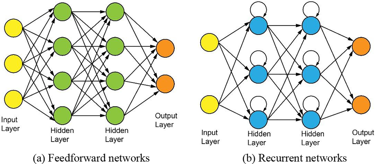
Figure 2: Schematic diagram of the main topologies of SNNs

Compared with the feedforward networks, recurrent SNNs add recurrent or feedback loops within the layers, as shown in Fig. 2b. The addition of these loops allows the output of the neuron to be influenced by the input in conjunction with the output of the previous moment, giving the network a memory function and the ability to extract connections between successive inputs. Thus, this kind of networks are suitable for processing contextual, sequence-like tasks. However, training large recurrent networks is also more difficult than the training of large feedforward networks due to the complexity of the structure.

Hybrid SNNs, on the other hand, contain both structures described above. Depending on the ease of implementation and training of the network, the most dominant are the feedforward SNNs.

3  Datasets

ANNs express information through precise floating-point numbers, only achieving information transfer in the spatial domain. In SNNs, on the other hand, information is input to neurons in the form of discrete spike sequences with precise timing. Currently, traditional image datasets such as MNIST [23] and CIFAR-10 [24] as well as neuromorphic datasets are mainly used in SNN research.

3.1 Traditional Image Datasets and Information Coding

Conventional image datasets consist of image samples constructed from pixels with continuous values. They need to be encoded into spike sequences in order to be input into the SNNs, and this process is called information coding. Therefore, what kind of spike sequence is encoded to express information is an important research direction in spiking neural networks. Since the terminology and classification methods used in many coding methods are often not uniform across publications, it is easy to confuse the difference between these coding schemes. For these coding methods, it is urgent to give a clear and effective categorization scheme. Therefore, in this paper, we categorize the current major information coding methods into three main categories, rate coding, time coding and trainable coding, based on whether the coding rules are set artificially, and whether the information is included in the specific timing of the spike. And the main information coding methods of SNNs are introduced from the perspective of serving SNN computing research.

3.1.1 Rate Coding

In rate coding the information is expressed mainly through the spike firing rate, which is the average number of spikes emitted by neurons within a certain sampling time. The larger the value to be expressed, the more spikes there are within the same sampling time window. The exact timing of spikes and the order between spikes do not determine the representation of the information in rate coding. The most common way to realize rate coding is to convert the value into the average rate of spike generation, i.e., the number of spikes emitted within each sampling time window [25]. The specific distribution of the spikes within the sampling time window can be done directly by means of equally spaced distribution, called count rate coding or frequency coding, as shown in Fig. 3. It can be also done by means of random distribution according to a probabilistic model, usually using the Poisson distribution model, which is known as Poisson coding.

Figure 3: Schematic diagram of rate coding

The rate coding is currently the most widely used coding method due to its simplicity, ease of operation, and strong robustness. Especially in the scenario of converting the trained ANN to SNN, the continuous output values in the ANNs can be directly regarded as the spike firing rate of the SNNs. However, because it adopts the sampling method of taking the mean value in the time window, it ignores a lot of detailed information on the time structure. This makes the information capacity of rate coding relatively insufficient, and a sufficiently long timing window needs to be guaranteed, which may require longer recording time or more neurons to be involved.

3.1.2 Temporal Coding

If the information conveyed by the neuron is contained in the specific moment of issuance of the spike, then such a coding method is known as temporal coding. That means that temporal coding uses differences in the structure of time as a carrier of information as well. There are many different types:

Time-to-first-spike Coding (TTFS): The information is encoded as the time difference Δt between the starting point of the excitation (i.e., the reference point) and the neuron’s first spike. Usually the larger the original value, the smaller the time difference Δt, i.e., the earlier the spike is issued [26]. There is no unique way of mapping real values to the TTFS, and the commonly used mapping functions include linear functions, reciprocal functions, logarithmic functions, and so on. TTFS is one of the most basic temporal coding methods.

Phase Coding [27]: In contrast to TTFS where the excitation start point is used as the reference point, phase coding encodes information based on the relative time difference between the spike and the reference oscillation.

Rank-Order Coding (ROC) [28]: The information is represented by the relative order in which the spikes are fired between neurons, so that rank-order coding does not actually require precise timing of the spikes.

Inter-Spike Interval Coding (ISI): Information is encoded into the relative time difference between successive spikes within a time window, also known as delay coding [29,30].

These temporal coding methods are summarized in Table 2 and their schematic diagram is shown in Fig. 4. In addition to the above methods, there are various kinds of temporal coding such as population-based temporal coding [30], temporal contrast coding (TCC) [31], etc., which will not be elaborated here.

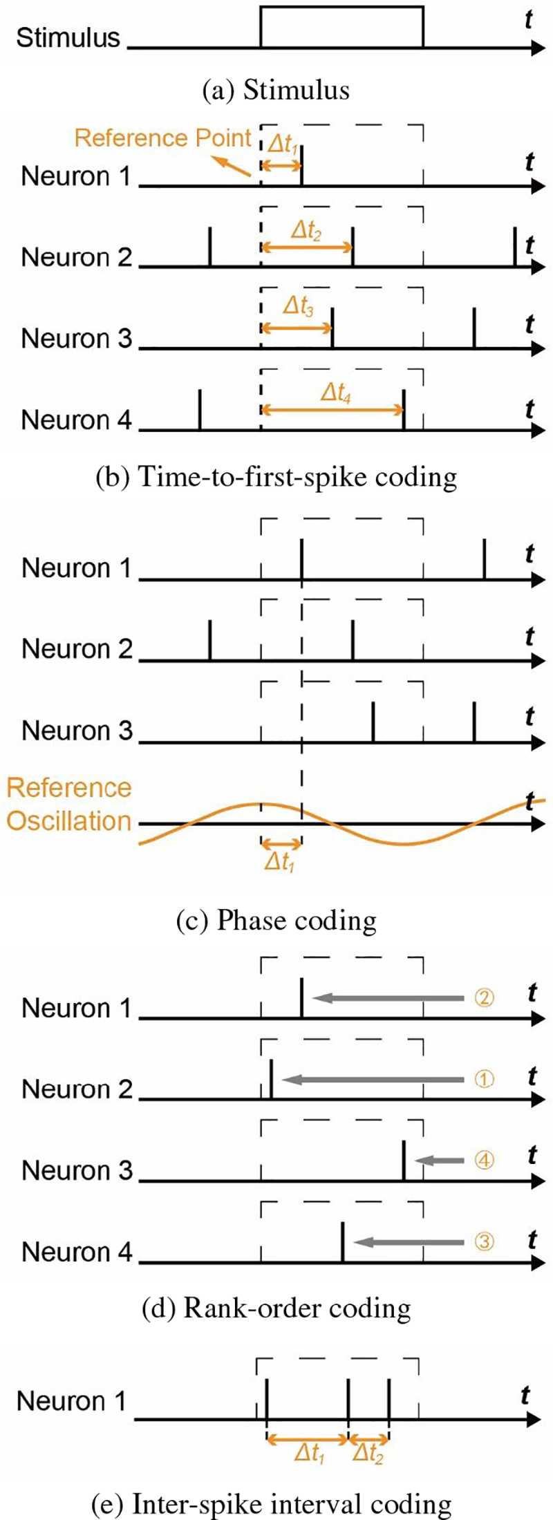
Figure 4: Schematic diagram of major time coding methods, adapted from the reference [30]

Compared to rate coding, temporal coding has higher information capacity, faster response time and higher transmission speed. In addition, temporal coding supports local learning rules and its temporal characteristics are closer to the information transfer mechanism in biological nerves. However, temporal coding also has disadvantages such as difficulty in implementation and sensitivity to noise. It is mainly used in shallow networks, and is not effective in larger-scale networks and datasets.

3.1.3 Trainable Coding

With the gradual development of deep SNNs, trainable coding has been proposed and rapidly gained wide application [32–34]. Trainable coding is also referred to as direct coding in some literature. Compared to rate encoding and temporal coding, which are manually formulated with specific encoding methods, trainable coding directly uses the first layer of the network as a coding layer, and transforms the input, real-valued image pixel into spiking output images. The specific process is shown in Fig. 5. The input image undergoes a layer of convolution operation. For T time steps of SNN, the above convolution operation is repeated T times. Subsequently, the convolution results are put into the spike neuron layer, and the excited neurons emit spikes. The weights in the encoding layer can then be trained along with the network.

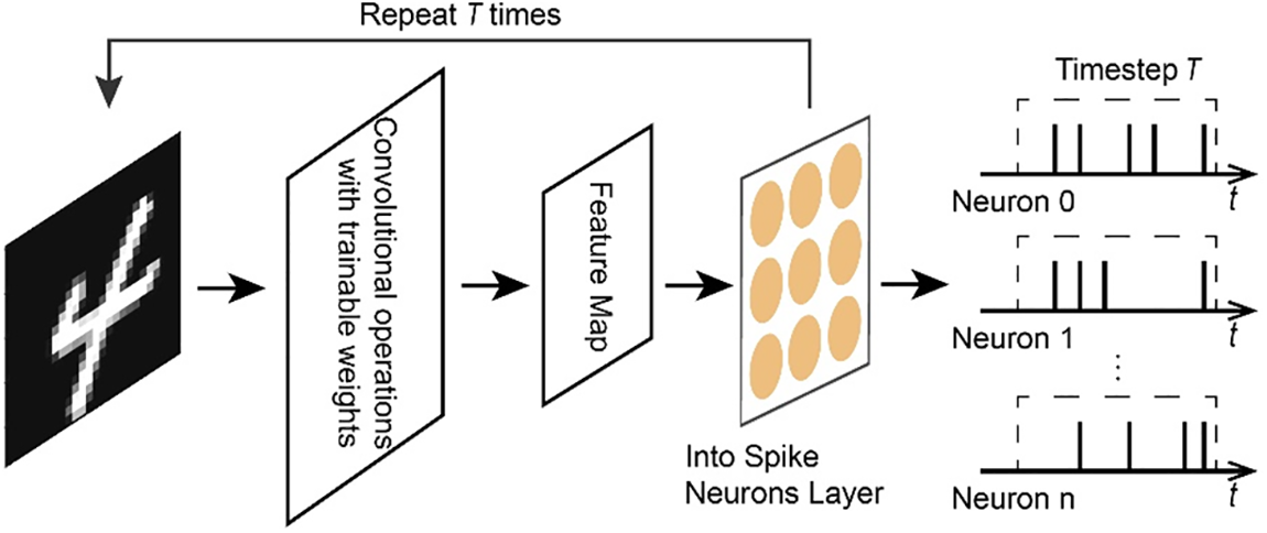
Figure 5: Schematic diagram of trainable coding

Trainable coding has demonstrated higher accuracy than rate coding in deep network structures because the loss function can be minimized by training. As a result, trainable coding has gained widespread attention and applications in recent years. And as the network gets deeper and the time step is set shorter, the accuracy advantage of trainable coding becomes greater. However, the robustness of trainable coding is still not as good as rate coding under adversarial and interference conditions [32]. In addition, because trainable coding is essentially a network layer with real-valued inputs, its implementation requires more energy and is more costly to deploy in hardware than rate coding and time coding, which have simpler rules.

Rate coding, temporal coding and trainable coding provide their own advantages and disadvantages, and it is necessary to flexibly choose based on these characteristics and specific application scenarios.

3.2 Neuromorphic Datasets

Although traditional image datasets are now widely used in SNN research, they lack information in the time domain and cannot fully utilize the spatio-temporal processing properties of SNNs. And these data need to be encoded into spike sequences before they can be used by SNNs, which may lose some information in the image. Therefore, applying SNNs to process new datasets with temporal information and SNN-compatible properties can more fully utilize SNNs’ advantages over ANNs. Among them, the datasets generated based on neuromorphic vision sensors, such as dynamic vision sensors (DVS), are considered to be one of the most suitable datasets for spiking neural network applications at present.

Conventional cameras output frame-based images. Neuromorphic vision sensor, on the other hand, is inspired by the neural structure of the retina. It captures only the brightness change of a single pixel and outputs a stream of spike events containing more temporal features. So it also called as event cameras. This is a natural fit with SNN’s characteristics. Whereas ANNs need to integrate these spike event streams into frame-based images when processing such datasets, losing the temporal information in them [35]. Such datasets mainly include datasets obtained from photographing traditional image datasets by DVS, such as N-MNIST [36], CIFAR10-DVS [37], datasets transformed from traditional images using software algorithms, like ES ImageNet [38], and datasets directly captured from real scenes using neural morphological visual sensors, such as the DVS128 Gesture [39], DVS Benchmark [40], DSEC [41]. Fig. 6 represents the images obtained by integrating the event stream in the DVS128 Gesture dataset over a certain period of time, which represent the gestures of rotating the arm up and down, clapping, and waving the left hand, respectively.

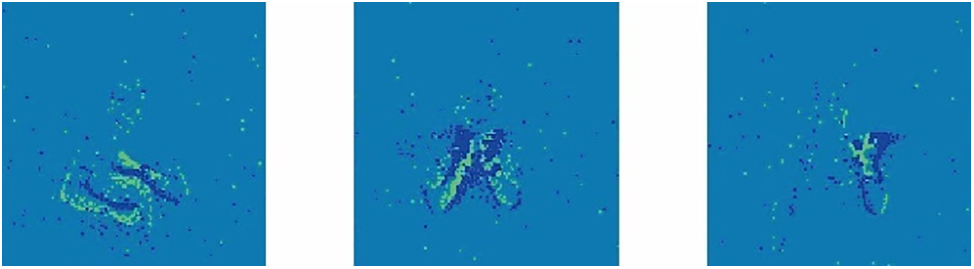
Figure 6: Schematic diagram of the DVS128-Gesture dataset

In addition, data from event-based audio sensor (like N-TIDIGITS dataset [42]), pulse activity recorded from real biological nervous systems, and other data also have the potential to be applicable to SNNs [43]. However, including datasets captured by neuromorphic visual sensors, these datasets are generally small in scale and there is no unified processing standard for them. This means that such datasets still need to be developed. Of course, some scholars have tried to apply small-sample learning methods in ANNs such as active learning [44] and transfer learning [45] to such datasets. For example, Wang et al. [46] used transfer learning to generate a transplanted network that can handle the neuromorphic dataset N-TIDIGITS from a network trained by the traditional audio dataset TIDIGITS [47].

4  Learning Algorithms

Compared to the training of ANNs, there are still many problems and challenges in the efficient training of SNNs, and there has not yet been a recognized optimal training method in the field of SNNs. According to different emphases such as computational performance or biological feasibility, as well as differences in network structure, there are currently many training methods for SNNs. The recent training methods have shown significant differences in focus and performance compared to early training methods, and the training results are still continuously improving. It is necessary to review and organize these training methods. These training algorithms can be mainly categorized into unsupervised learning algorithms and supervised learning algorithms.

4.1 Unsupervised Learning

Unsupervised learning algorithms use unlabeled datasets, rely on the network itself to learn the features and associations in the data, and adaptively adjust the synaptic weights of neurons to complete the functions of recognition and classification. The unsupervised learning methods in SNNs are mainly centered around the Spike Timing Dependent Plasticity (STDP) rule [48,49].

The STDP rule is a manifestation of Hebb’s learning rule [50], which describes the following phenomenon found in the brain: the connection between two linked neurons will be strengthened if the presynaptic neuron also emits spikes shortly before the firing of the postsynaptic neuron. On the contrary if the presynaptic neuron emits spikes shortly after postsynaptic neuron emits spikes, the connection strength between them will be reduced. That is to say, the logic that exists in time will determine the direction and magnitude of synaptic changes. The neurons that have a strong forth-and-back relationship will strengthen the connection, and vice versa, they will drift away from each other, so as to establish the connection with sequential relationship. The STDP rule uses the time difference between the activation of the two neurons to update the neuron weight. The typical mathematical model of the STDP rule is as follows:

Δw={A+exp(Δtτ+),ifΔt<0−A−exp(−Δtτ−),ifΔt≥0,Δt=tpre−tpost(5)

where Δw is the amount of weight change, τ+ and τ− are the time window constants, A+ and A− are the gain of weight enhancement and attenuation, respectively. And tpre and tpost are the spike firing moments of the presynaptic neuron and postsynaptic neuron, respectively.

The STDP rule can effectively reflect biological characteristics and is one of currently the most widely used unsupervised learning method for SNNs. It is the training method that can best demonstrate the higher biological plausibility of SNNs compared to ANNs. Several studies have proposed variants of STDP, such as anti-STDP [51], Triplet-STDP [52] and Stable-STDP [53]. However, due to the dependence on the connection between each layer and its previous layer, STDP lacks the ability to effectively coordinate with other parts of the network, and has poor classification performance in multilayer network structures. Thus, its application is mainly limited to shallow networks. In order to improve the recognition accuracy of STDP in real-world problems, some related studies have used STDP rules in combination with other methods like layer-by-layer training, Winner Take All (WTA). For example, Kheradpisheh et al. [54] and Paredes-Valles et al. [53] used such methods to achieve unsupervised learning in three-layer networks. Tavanaei et al. [55] applied STDP with spike sparse self-encoder in layer-by-layer greedy training. Li et al. [56] adopted a multilayer network with a locally-connected structure and trained the network using STDP method combined with the spatial and temporal information-based neuron adaptive activation mechanism. All these schemes achieved more satisfactory results on the MNIST dataset.

4.2 Supervised Learning

Supervised learning algorithms rely on labeled datasets and compare the error between the output results and the actual labels to update the weights. In this paper, we will categorize the main SNNs supervised learning methods from the perspective of algorithmic principles.

4.2.1 Learning Algorithms Based on Biological Synaptic Plasticity

Biological synaptic plasticity rules such as STDP belong to unsupervised learning algorithms and are applicable to limited scenarios, so they need to be generalized to supervised learning. An early typical representative is the remote supervised method (ReSuMe) [57], proposed by Ponulak et al. This algorithm combines the STDP rule with remote supervision, and adjusts the synaptic weights through the combination of STDP and anti-STDP, so that the neuron output is as close as possible to the desired spike signal. The algorithm mainly uses the correlation between the desired spike signal and the input signal, and there is no direct physical connection between the desired signal and the output signal of the trained neurons, which reflects its “remote supervision”. ReSuMe has online learning capabilities that can be applied to various neuron models and can process spike series, but it only supports single neuron or single-layer network. Sporea et al. proposed Multi-ReSuMe algorithm [58], which extends the ReSuMe algorithm to multilayer feedforward SNNs.

Some scholars have also combined STDP with other biological mechanisms such as forgetting phenomenon and reward regulation, such as Li et al. [59] applied forgetting phenomenon in STDP to improve the training recognition rate and accelerate the convergence speed. Mozafari et al. [60] combined STDP rules with reward and punishment signals to train SNNs. While one approach widely adopted in the current research is to train different layers of the network separately by STDP and other supervised learning methods to deepen the number of layers of the network. Lee et al. [61] initialized the weights of the network by STDP and then used gradient descent method to fine-tune the synaptic weights to complete the training of the network. Xu et al. [62] proposed a hybrid network of convolutional neural networks (CNNs) and SNN, called Deep CovDenseSNN, and used a hybrid training method of error backpropagation to train the convolutional layer and STDP to train the SNN part. Shao et al. [63] proposed a joint learning method called excitatory inhibition loop iterative learning (EICIL), where STDP is used as an inhibitory mechanism and gradient backpropagation is used as an excitatory mechanism to train the convolutional layer and the other layers, respectively, in order to realize deep SNNs with higher biological plausibility.

4.2.2 Learning Algorithms Based on Gradient Descent

Bohte et al. applied the ideas of error backpropagation and gradient descent to simplified SRM models and proposed the SpikeProp algorithm [64], which was one of the earliest supervised learning methods used for spike neurons. SpikeProp supports a multilayer feedforward network with SRM neurons. To overcome discontinuities in the internal state variables of spike neurons, the method approximates the threshold function and restricts all neurons in the SNN to fire only a single spike. Since then, many researchers have proposed variant algorithms of SpikeProp to improve its limitations in different ways, such as Multi-SpikeProp [65], SpikeProp Through Time (SPTT) [66], etc. Tempotron [67] is another early gradient descent-based SNN learning algorithm. The algorithm uses gradient descent for the error function of membrane potential vs. threshold potential to adjust the synaptic transmission efficiency to realize binary classification. Despite the high biological plausibility of this method, it is only applicable to a single spike with a single neuron, which greatly limits its application. Then Florian proposed the Chrontron [68] algorithm based on Tempotron, which can train the monolayer network with spike sequences.

With the great achievements of error backpropagation (BP) and gradient descent in deep learning in recent years, the idea of applying gradient descent directly to SNNs has received renewed attention. To solve the problem that the error function is not continuously differentiable, the surrogate gradient method (also called gradient approximation) has been widely adopted in recent years and has gradually become one of the current mainstream direct training methods for SNNs. Therefore, unless otherwise indicated as early gradient descent methods, the terms gradient descent method and direct training method in the following text both refer to various training algorithms based on gradient descent with gradient approximation. As shown in Fig. 7, the core idea of the surrogate gradient method is to approximate the non-differentiable activation function of spike neurons, H(x), with a similar shape but smooth differentiable function [69], S(x). The algorithm uses the original activation function in forward propagation, while in backward propagation, it replaces the gradient of the original non-differentiable activation function with the gradient of the surrogate function, S′(x). For example, the Spike Layer Error Reassignment (SLAYER) training method proposed by Shrestha et al. [70] combines gradient approximation with temporal credit assignment. Wu et al. proposed the Spatio-Temporal Backpropagation (STBP) [71] training method, which combines the layer-by-layer spatial and temporal domain information to train the network. They also introduced four approximation curves of the SNN’s gradient for error backpropagation. STBP offered the possibility of investigating high-performance SNNs that can handle neuromorphic datasets with complex spatiotemporal properties. Lee et al. [72] proposed an approximate derivative algorithm to account for the leakage behavior of the LIF neurons and implemented the training of SNNs that reached VGG9 or ResNet11 structures.

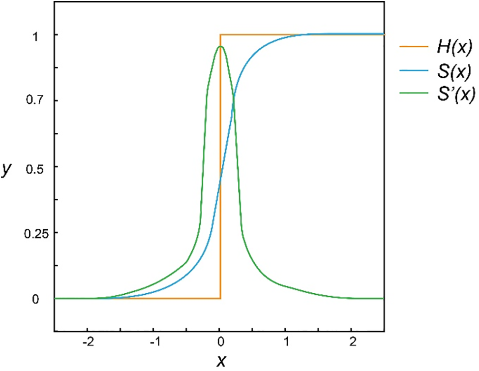
Figure 7: Schematic diagram of the surrogate gradient

However, there are some problems with the surrogate gradient method. there is an obvious gradient mismatch between the gradient of the excitation function and the surrogate gradient [73], which easily leads to under-optimization of SNNs and serious performance degradation. And the problem of exploding or vanishing gradients is still serious. This makes SNNs only relied on surrogate gradient training remain in shallow structures and difficult to apply on large datasets (such as ImageNet [74]). However, the ability demonstrated by deep neural networks also made researchers eager to find suitable training methods for deep SNNs. Zheng et al. proposed a batch normalization method called threshold-dependent Batch Normalization (tdBN) [75] based on the STBP method, which to some extent avoided the problem of gradient vanishing or exploding during training. They increased the number of trained network layers from less than 10 to 50, and for the first time achieved direct training of large-scale SNNs on ImageNet. Fang et al. [76] proposed a residual SNN structure called Spike Element Wise (SEW) ResNet to alleviate the model degradation problem when directly training ultra-deep networks, and directly trained a network model with more than 100 layers for the first time. Feng et al. [77] designed the Multi-Level Firing (MLF) method based on the STBP and proposed the spiking dormant-suppressed residual network (spiking DS-ResNet), which effectively solves the problem of gradient vanishing and network degradation when directly training deep SNNs. Deng et al. proposed the Temporary Efficient Training (TET) algorithm [78], which improved the generalization ability of SNNs by compensating for momentum loss during gradient descent, and further improved the training performance on datasets such as ImageNet and CIFAR10-DVS.

With the continuous improvement of the training effect, SNN models trained with gradient descent are becoming more and more diverse. In object detection tasks, the YOLO series is one of the most classic models. Su et al. [79] proposed the first directly trained spiking YOLO network structure, Energy-efficient Membrane-Shortcut-YOLO (EMS-YOLO), based on the residual module with a full spike structure, and successfully applied it in the object detection task. Recently, the large language model has received a lot of attention and it is based on Transformer architecture and self-attention mechanism. So combining them with SNNs has become a recent research hotspot. Zhou et al. [80] proposed the Spiked Self-Attention (SSA), which uses sparse spikes to represent the query, key, and value of the self-attention mechanism, Based on this, they designed a spike-based transformer, Spikformer, and for the first time implemented the self-attention mechanism and Transformer architecture in directly-trained SNNs. Wang et al. [81], on the other hand, proposed a spatio-temporal self-attention (STSA) mechanism that captures dependencies from both temporal and spatial domains while maintaining the asynchronous information transmission capability of SNNs. Based on this, they developed the spatio-temporal spiking transformer (STS-Transformer) architecture, which achieved breakthrough results of SNNs on speech datasets. The integration of many excellent network architectures in ANNs into SNNs significantly increases the information capacity of SNNs and thus improves the performance of SNNs.

4.2.3 Indirect Learning Algorithm Based on ANN Conversion

With the rise of deep learning, there are also more and more scholars nowadays who utilize the mature learning algorithms of ANNs to train SNNs indirectly. Such schemes firstly perform backpropagation training in a designed ANN, and subsequently transform the trained ANN into a similarly structured SNN, to circumvent the difficulties faced by the direct training of SNNs. This utilizes the strong similarity between the spike firing rate of IF neurons in SNNs and the nonlinear activation of ReLU functions in ANNs. Of course, to achieve ANNs conversion to SNNs and minimize performance loss, certain constraints need to be placed on the original ANN, such as using only the ReLU function, disabling bias, not being able to use batch normalization and maximum pooling, and needing to normalize different layers of the network.

The method of converting ANN to SNN (hereafter referred to as the ANN conversion method) has strong scalability, making it easy to convert newly emerging large-scale ANN network structures into corresponding SNN versions, enabling large-scale deep spike neural networks and processing large-scale datasets. Sengupta et al. [82] for the first time achieved 69.96% accuracy of SNNs on complete ImageNet datasets through the method of converting SNNs by ANNs, implemented an SNN network based on ResNet architecture, and explored the conversion of ANN to SNN for event-driven operations to reduce computational overhead. Hu et al. [83] achieved the construction of a spike ResNet network with more than 100 layers by scaling the continuous-valued activations in the ANNs to match the firing rate in the SNNs and proposing a compensating mechanism to reduce the error caused by discretization.

Although many papers have now demonstrated the ability of the ANN conversion method to achieve state of the art (SOTA) classification performance. However, its essence is to perform backpropagation in ANNs to circumvent problems such as non-differentiable neuron equations encountered by backpropagation in SNNs. The constraints imposed on the original ANN will inevitably result in performance degradation compared to the original ANN. The converted SNN requires longer time steps compared to networks trained by the gradient descent method, which is inefficient. It cannot be applied to online learning methods, which cannot achieve continuous learning and real-time adaptation. In addition, it is difficult to extract the temporal dimension features from the ANN training, and thus the method is not yet applicable to spatio-temporal data classification. At present, many scholars have begun to focus on solving these problems of ANN conversion method methods. For example, Kugele et al. [84] introduced the Streaming Rollouts method [85] in the process of ANN conversion, so that the generated SNN can effectively integrate temporal information, and ultimately achieve good results on neuromorphic datasets. Li et al. [86] proposed lateral inhibition pooling and a neuron model that releases bursts of spikes to reduce the maximum pooling output error and the residual information error in the conversion process, respectively. The former is an important reason why the transformation method cannot use maximum pooling. Bu et al. [87] optimized the initial membrane potential of spike neurons to reduce the conversion loss at each layer of the network, and realized a nearly lossless ANN conversion or significantly improved the performance at low inference time steps.

From the above, it is easy to see that in the last decade, the development and prosperity of deep neural networks have also exerted great influence on the research of SNNs. Many structures, learning algorithms, and ideas of ANNs have been introduced into SNNs, making the performance pursuit and application scenarios of SNNs computation in recent years very different from those in the early days. The summary of early SNNs supervised learning methods and the summary of SNN learning methods in recent years described in the previous section are shown in Tables 3 and 4, respectively. As can be seen from Table 4, more and more researchers in the SNN learning algorithm field in the last two years have started to use SNNs to challenge large-scale datasets such as CIFAR100, ImageNet, etc. SNN learning algorithm research has also started to concentrate on these two methods, namely, indirect training based on the ANN conversion and direct training based on the gradient descent. Among them, the performance of the ANN conversion method has been further improved. In addition to improving the recognition accuracy, other objectives like reducing the conversion loss, inference step size, and constraints have also been paid more attention. In the past two years, many SNN learning algorithms based on gradient descent have also developed the ability to challenge large datasets such as ImageNet and achieved good results. Meanwhile, thanks to the spatio-temporal information processing capability of training methods such as STBP, the deep SNNs trained by these methods is more suitable for processing neuromorphic datasets compared to ANNs as well as SNNs trained by ANN conversion methods. The performance of SNNs trained by these methods has made significant progress in neuromorphic datasets such as CIFAR10-DVS. Overall, these two methods have gradually become the mainstream SNN learning algorithms in recent years, and they are also the two algorithms with the best performance on real tasks. The emergence of these two learning algorithms also promotes the development of SNNs towards deeper network structures and higher performance.

5  Software and Hardware Platforms

The reason why deep learning has been able to achieve rapid development and land in various industries in recent years, cannot be separated from various deep learning frameworks represented by Tensorflow and PyTorch. For the large amount of arithmetic power demand brought about by neural network development, hardware platforms represented by artificial intelligence (AI) hardware accelerators such as NVIDIA A100, GOOGLE TPU, and AI units integrated in various types of SoCs (System on Chip), provide a reliable guarantee for the actual landing of ANNs in various types of devices from the data center to the edge side. However, in the field of SNNs, the current software programming frameworks and specific hardware platforms are still in the early stage of development, providing different functionalities and covering different scenarios. This increases the development difficulty of SNNs and restricts the application and promotion of SNNs. Therefore, reviewing and organizing existing software programming frameworks and specialized hardware platforms is of great help in selecting suitable platforms and applying SNNs in practical applications.

5.1 Software Programming Frameworks

There are a variety of programming frameworks in the SNN field, but the overall development level is in the early stages, and the focus of the application scenarios of these frameworks is also different. Some SNN frameworks are mainly applied to realize the functional simulation and behavioral simulation of neurons and small-scale network models, i.e., the main goal is to understand the mechanisms of biological systems. These frameworks include Neuron [88], Genesis [89], Nest [90], Brian2 [91], Nengo [92], GeNN [93], etc. Neuron and Genesis are mainly based on C or C++ and also provide visual interfaces that can be used to achieve precise simulation of neuronal behavior models, such as multi-compartment neuron models, modeling of multiple synaptic types, and so on. Nest, Brian2, and Nego are mainly developed in Python language. In addition to supporting neural simulation, they also support various neural network-level simulations, as well as SNN learning algorithms such as STDP, and even have a certain degree of machine learning ability. GeNN, on the other hand, is written in C and C++ language based on CUDA, to implement the simulation of SNNs using GPU.

The other part of the SNN framework mainly focuses on the realization of machine learning tasks and large-scale SNN computing, such as BindsNet [94], SpyKetorch [95], Norse [96], snnTorch [97] and SpikingJelly [98] and so on. Such platforms can accelerate the construction of SNNs in tasks such as bionic learning, supervised learning, etc., and can support SNN applications in scenarios such as image classification and speech recognition. This kind of platform can support many kinds of training algorithms such as STDP. Emerging development platforms such as NengoDL (a variant of Nengo), Norse, snnTorch, and SpikingJelly can even support deep learning algorithms like gradient descent methods or ANN conversion methods. Most of such frameworks are extended from current mainstream deep learning platforms such as Tensorflow, Pytorch, etc., and integrate SNN representation, computation, and other functions into these platforms. An example is the SpikingJelly framework shown in Fig. 8. Therefore, such SNN frameworks can directly utilize the existing resources and optimization techniques of these deep learning platforms, such as using the tensor calculation of the deep learning platform to model SNNs to make it easier to use the framework, and using parallel processing extensions like NVIDIA’s CUDA to significantly increase the simulation speed [99].

Figure 8: Architecture diagram of SpikingJelly [98]

In addition to the different focuses of the application scenarios, these SNN frameworks differ in their simulation computation methods, which can be roughly categorized into event-driven, clock-driven, and hybrid-driven types. In clock-driven frameworks, a time step is required to be set for each iteration, and the state of each neuron is computed and updated at each time step according to the input at that time [100]. In the event-driven mode, the state update of neurons is triggered by spike events, so the activities of different neurons can be calculated asynchronously. So, there is no need to calculate the state of neurons at every moment. Hybrid-driven types include both event-driven mode and clock-driven mode. Due to the lower implementation difficulty, most frameworks are currently time-driven. And time-driven mode has high parallelism, which can make full use of the parallel resources of CPU and GPU, and is suitable for scenarios like triggering a large number of events and simulating large-scale networks. While the asynchronous nature of event-driven makes its simulation faster and more suitable for neural network layers with low and sparse activity. However, due to the sequential nature of the event-driven way, it is difficult to parallelize the execution of event-driven simulation through current mainstream hardware platforms [101]. The above SNN programming framework is summarized in Table 5.

5.2 Dedicated Hardware Platforms

ANNs are good at handling problems of dense data, high-precision requirements, and insensitive to computing cost, while SNNs are good at handling problems of sparse data, low accuracy requirements, and low computing costs. The difference between the two leads to different design ideas for the corresponding hardware acceleration platform. For the implementation of SNNs, it is usually inefficient to execute SNNs on the traditional von Neumann architecture CPU, while the GPU architecture is incompatible with the event-driven asynchronous mechanism of SNNs, which fails to fully utilize the low-power advantage of asynchronous processing in SNNs. Therefore, it is necessary to design hardware architectures for SNNs based on the above characteristics to fully utilize the event-driven, low-power characteristics of SNNs. In recent years, many scholars have proposed a series of SNN-specific hardware acceleration chips, which are often called neuromorphic chips. To achieve the characteristics of SNNs, these neural morphology chips can simulate the cell dynamics and synaptic memory of spike neurons and are designed in an event-driven manner, which triggers the state update of neurons through spike events. To support the realization of SNNs with different structures and scales, neuromorphic chips need to be highly configurable and scalable. Such hardware platforms usually utilize multi-core architectures based on the Network on Chip (NoC). A typical neuromorphic chip architecture is shown in Fig. 9. The computational cores are the basic units of the architecture, which can be configured to simulate a certain number of neurons and synapses. Each computational core has an independent memory and can operate independently without relying on a unified external memory, thus improving parallelism, avoiding large memory accesses, and breaking the memory bottleneck in traditional von Neumann architectures [102]. These independent computational cores are combined with routing units to access the NoC, which accomplishes the data communication among the compute cores. Such an architecture can be implemented on a single chip, and can also be deployed in chipsets to implement larger-scale neural networks in combination with multi-chip interconnections.

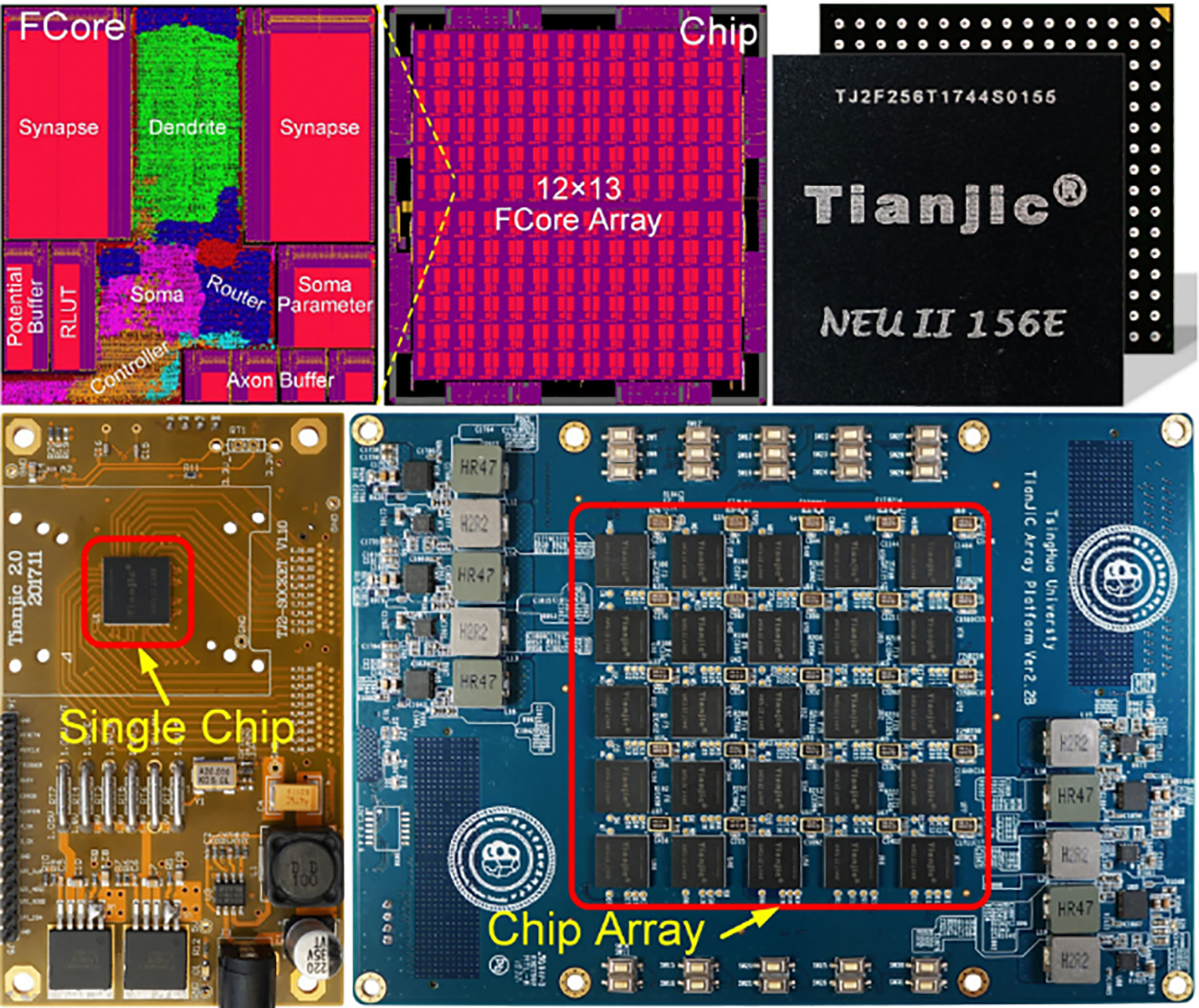
Figure 9: Schematic diagram of neuromorphic chip architecture, taking Tianjic [103] as an example

According to the different ways of circuit implementation, these hardware platforms can also be classified into hybrid digital-analog platforms and all-digital platforms. For hybrid digital-analog computing platforms, since most of the neuron models are presented in the form of differential equations, analog circuits can be used directly to simulate the cellular dynamics of spike neurons through the current-voltage characteristics of transistors in the subthreshold or suprathreshold state. The routing unit and interconnecting network need to ensure that the data can be transmitted stably over long distances, so this part needs to be completed using digital circuits which are more stable and reliable compared to analog circuits. The hybrid digital-analog platforms use analog computation to achieve low power consumption and fast response time. For all-digital platforms, although their power consumption is higher than that of hybrid digital-analog solutions, they can flexibly adjust the SNN structure and parameters through compatible programming software and are more design-convenient and stable. They can even be achieved using the latest advanced process. Therefore, all-digital computing platforms are more favored in the industry.

Representative neuromorphic chips include BrainScaleS-2 [104] from Heidelberg University, DYNAPs [105] from the University of Zurich, Neurogrid [106] from Stanford University, TrueNorth [107] from IBM, Loihi-2 [108,109] from Intel, Zhejiang University’s Darwin-2 [110–112] and Tsinghua University’s Tianjic [103] and so on. among them, BrainScaleS-2, Darwin-2 and Loihi-2 are their respective second-generation hardware platforms that have been made public in recent years. In addition, most research institutions operating these platforms have built their own system-level neuromorphic hardware platforms based on the aforementioned chips in the form of multi-chip interconnection. To make it easier to develop SNNs on these platforms, some of them provide dedicated programming frameworks and model compilers to improve the programmability of the hardware platform [113]. Taking Loihi as an example, Intel has introduced the supporting software toolchain, Lava, which greatly improves the ease of use of the Loihi platform and allows researchers to deploy SNNs in a variety of application scenarios, such as neuromorphic data processing [114], proportional-integral-differential (PID) [115] closed-loop control [116,117], and so on.

The hardware platforms mentioned above are larger-scale platformed specific SNN hardware accelerators. The specifications and comparisons of these platforms can be found in Table 6. Their design concepts and system architectural features enable the system to be configured and used for a wide range of tasks and operating modes, i.e., they are general-purpose platforms designed specifically for SNNs. Besides, there are numerous small-scale SNN hardware designs aimed at hardware acceleration of SNNs in low-power scenarios, e.g., ASIC-based designs such as ODIN from the University of Leuven [118], ReckOn from the University of Zurich [119], as well as designs based on FPGA implementations [120–122]. Such hardware is only capable of running smaller scale networks for simple tasks, and can only support limited network types or even only realize fixed network topologies. Therefore, most of them do not have complex supporting software kits. In recent years, utilizing the in-memory computing characteristics of memristor arrays has also become a promising approach to achieving SNNs. This type of design utilizes memristors to achieve synaptic storage and integration operations in the analog domain, such as works [123–125] and so on. However, due to the non-idealities of the device, the current SNN systems based on memristors are very simple, and there is still a long way to go for being practical.

6  Conclusions and Future Perspectives

This paper comprehensively introduces the current research results and possible future development directions of SNNs from four aspects: the composition structure of SNNs, datasets, learning algorithms, and software/hardware development platforms.

In terms of network composition structure, this article mainly introduces the neuron models such as the IF model, LIF model, and SRM model, and the functions of neuron synapses, as well as three main network topology structures. In terms of the dataset used in SNNs, this article introduces the two types of information coding methods required for using traditional image datasets: rate coding and temporal coding, as well as neuromorphic datasets that are more suitable for SNNs. In terms of learning algorithms, the main learning algorithms in SNNs such as STDP rules, gradient descent algorithms for SNNs, ANN conversion method, and so on are summarized from two perspectives of unsupervised learning and supervised learning, and the advantages and disadvantages of these algorithms are analyzed. In terms of software and hardware development platforms, this article introduces the development achievements of several major SNN programming frameworks and neuromorphic hardware platforms.

Comprehensively analyzing the research progress of SNNs in various aspects, we can see that the current development of SNNs is not yet perfect and there are still many problems to be solved.

In terms of information coding, the challenge still to be solved is how to better realize the spike coding of information. Information coding has a significant impact on the realization and performance of SNNs, so it is necessary to find a suitable coding strategy as well as a learning algorithm that matches it. On the other hand, most of the current deep SNNs use rate coding, which restricts SNNs from utilizing their advantages in processing temporal-domain information. How to fully integrate temporal coding with larger information capacity and higher transmission speed with deep SNNs is also a direction to be explored.

In terms of construction and training of models, with the rise of large-scale models, how to build SNNs with more complex structures, larger scale, and richer application scenarios, and successfully train them, will be an important research direction to make SNNs more practical. This requires researchers to explore how to design SNN network structures that have stronger information extraction and representation capabilities and are easier to train. This issue also requires improving the effectiveness of current training algorithms in dealing with such sophisticated networks. However, learning algorithms like the backpropagation algorithm, which has gained recognized results in ANNs, have not yet been developed in the field of SNNs. At present, the two methods, the surrogate gradient method and ANN conversion method, have achieved numerous results. SNNs trained based on these methods still has a certain gap with ANNs in terms of network depth and performance. The former still has not well solved the problem of gradient disappearance or gradient explosion in deep network training. The ANN-converted method cannot fully utilize the ability of SNNs to process temporal information, and the simulation step length is too long, which reduces its efficiency. Both algorithms still have much room for development. On the other hand, in terms of biological plausibility, there is still a need to further bridge the gap between neuroscience and intelligent computing. For example, how to enrich the dynamic model of spike neurons currently used in deep SNNs to improve the representative ability of neurons. Secondly, neither of these two training methods mentioned above has good biological plausibility. How to utilize biological rational learning methods, such as STDP rules, to train high-performance SNNs. These problems remain to be important challenges.

In terms of datasets, information coding is only a conversion method for traditional picture datasets applied in SNNs, and traditional picture datasets still lack sufficient temporal information for SNNs. Datasets with rich dynamic temporal information and natural pulse forms are more suitable for SNNs, but the size of such datasets is currently very small and still needs to be developed. In addition, most of the datasets used for SNNs at this stage are focused on image recognition scenarios, and more datasets in different scenarios need to be extensively explored to improve the diversity of SNN functions.

In terms of software development tools, classic software frameworks focus on neuroscience rather than deep learning, while frameworks applicable to deep learning are still in the early stages of iteration. The modules and APIs of these software are not yet stable enough and the functions covered are not comprehensive enough. In addition, these software frameworks are usually designed for CPUs and GPUs and lack support and optimization for different SNN hardware acceleration platforms. On the other hand, due to the temporal dimension of SNNs, these frameworks require a longer running time compared to ANNs when performing SNN training and inference, and the running efficiency of the frameworks needs to be further improved.

In terms of neuromorphic hardware, researching chip architectures that are more efficient and better utilize the asynchronous characteristics of SNNs is an important direction for future development. Among them, how to support more on-chip learning methods, how to be compatible with both ANNs and SNNs paradigms, and how to be integrated with neuromorphic sensors are all important challenges for the research of neuromorphic chip architecture. Developing neuromorphic chips through the in-memory computing characteristics of new memory devices, such as memristors, is also a very promising direction for the realization of SNN hardware acceleration in the future. But it is also urgently necessary to minimize the adverse effects caused by the non-idealities of the devices themselves.

Generally speaking, many development achievements in recent years have greatly improved the practicability of SNN computing, making it possible to apply SNNs to real-world problems. These problems mentioned above will be the focus of future research on SNNs. It is expected that in the current research boom of artificial intelligence, SNNs can break through the barriers between artificial intelligence and biological neuroscience, and realize the cross-fusion of the two. We hope that the development of SNNs can bring the development of brain-like computing to a new stage, provide more insights for humans to understand neuroscience, and provide a new paradigm for artificial intelligence.

Acknowledgement: All authors sincerely thank all organizations and institutions that have provided data and resources. Thanks to all the members of our research group, their suggestions and support have provided important help and profound impact on our research work.

Funding Statement: This work is partly supported by the National Natural Science Foundation of China (Nos. 61974164, 62074166, 62004219, 62004220, and 62104256).

Author Contributions: The authors confirm contribution to the paper as follows: study conception and design: Jiadong Wu, Yinan Wang, Zhiwei Li and Qingjiang Li; data collection: Jiadong Wu and Lun Lu; analysis and interpretation of results: Jiadong Wu and Yinan Wang; draft manuscript preparation: Jiadong Wu. All authors reviewed the results and approved the final version of the manuscript.

Availability of Data and Materials: Not applicable.

Conflicts of Interest: The authors declare that they have no conflicts of interest to report regarding the present study.

References

1. K. Shankar et al., “Synergic deep learning for smart health diagnosis of COVID-19 for connected living and smart cities,” ACM. T. Intsernet Techn., vol. 22, no. 3, pp. 1–14, 2022. doi: 10.1145/3453168. [Google Scholar] [CrossRef]

2. S. Li et al., “False alert detection based on deep learning and machine learning,” Int. J. Semant. Web. Inf., vol. 18, no. 1, pp. 1–21, 2022. doi: 10.4018/IJSWIS. [Google Scholar] [CrossRef]

3. R. A. Sobbahi and J. Tekli, “Comparing deep learning models for low-light natural scene image enhancement and their impact on object detection and classification: Overview, empirical evaluation, and challenges,” Signal Process.-Image, vol. 109, no. 12, pp. 116848, 2022. doi: 10.1016/j.image.2022.116848. [Google Scholar] [CrossRef]

4. M. Afify, M. Loey, and A. Elsawy, “A robust intelligent system for detecting tomato crop diseases using deep learning,” Int. J. Softw. Sci. Comp., vol. 14, no. 1, pp. 1–21, 2022. doi: 10.4018/IJSSCI. [Google Scholar] [CrossRef]

5. T. Brown et al., “Language models are few-shot learners,” in 2020 Neural Inf. Proces. Syst. (NeurIPS), Dec. 6–12, 2020, pp. 6–12. [Google Scholar]

6. D. D. Cox and T. Dean, “Neural networks and neuroscience-inspired computer vision (review),” Curr. Biol., vol. 24, no. 18, pp. R921–R929, 2014. doi: 10.1016/j.cub.2014.08.026. [Google Scholar] [PubMed] [CrossRef]

7. J. D. Nunes, M. Carvalho, D. Carneiro, and J. S. Cardoso, “Spiking neural networks: A survey,” IEEE Access, vol. 10, no. l, pp. 60738–60764, 2022. doi: 10.1109/ACCESS.2022.3179968. [Google Scholar] [CrossRef]

8. N. Burkitt, “A review of the integrate-and-fire neuron model: I. Homogeneous synaptic input,” Biol. Cybern., vol. 95, no. 1, pp. 1–19, 2006. doi: 10.1007/s00422-006-0068-6. [Google Scholar] [PubMed] [CrossRef]

9. W. Gerstner and W. M. Kistler, “Leaky integrate-and-fire model,” in Spiking Neuron Models: Single Neurons Populations Plasticity, 1 ed., Cambridge, UK: Cambridge University Press, 2002, pp. 94–96. [Google Scholar]

10. B. Rueckauer, I. Lungu, Y. Hu, M. Pfeiffer, and S. Liu, “Conversion of continuous-valued deep networks to efficient event-driven networks for image classification,” Front. Neurosci., vol. 11, no. 11, pp. 682, 2017. doi: 10.3389/fnins.2017.00682. [Google Scholar] [PubMed] [CrossRef]

11. E. M. Izhikevich, “Which model to use for cortical spiking neurons?,” IEEE. T. Neural Netw., vol. 15, no. 5, pp. 1063–1070, 2004. doi: 10.1109/TNN.2004.832719. [Google Scholar] [PubMed] [CrossRef]

12. W. Fang et al., “Incorporating learnable membrane time constant to enhance learning of spiking neural networks,” in 2021 IEEE Int. Conf. Comput. Vision, Montreal, France, Oct. 10–17, 2021. [Google Scholar]

13. Q. Yu et al., “Constructing accurate and efficient deep spiking neural networks with double-threshold and augmented schemes,” IEEE. T. Neur. Net. Learn., vol. 33, no. 4, pp. 1714–1726, 2022. doi: 10.1109/TNNLS.2020.3043415. [Google Scholar] [PubMed] [CrossRef]

14. Y. Wang, M. Zhang, Y. Chen, and H. Qu, “Signed neuron with memory: Towards simple, accurate and high-efficient ANN-SNN conversion,” in 2022 Int. Joint Conf. Artif. Intell. (IJCAI), Vienna, Austria, Jul. 23–29, 2022. [Google Scholar]

15. S. Kim, S. Park, B. Na, and S. Yoon, “Spiking-YOLO: Spiking neural network for real-time object detection,” in 2019 AAAI Conf. Artif. Intell. (AAAI), Honolulu, HI, USA, Jan. 27–Feb. 1, 2019. [Google Scholar]

16. W. Ye, Y. Chen, and Y. Liu, “The implementation and optimization of neuromorphic hardware for supporting spiking neural networks with MLP and CNN topologies,” IEEE T. Comput. Aid. D., vol. 42, no. 2, pp. 448–461, 2023. doi: 10.1109/TCAD.2022.3179246. [Google Scholar] [CrossRef]

17. W. Gerstner, W. M. Kistler, R. Naud, and L. Paninski, “Adaptation and firing patterns,” in Neuronal Dynamics: From Single Neurons to Networks and Models of Cognition, 1 ed., Cambridge, UK: Cambridge University Press, 2014, pp. 154–164. [Google Scholar]

18. W. Gerstner, R. Ritz, and J. L. Hemmen, “Why spikes? Hebbian learning and retrieval of time-resolved excitation patterns,” Biol. Cybern., vol. 69, no. 5, pp. 503–515, 1993. doi: 10.1007/BF00199450. [Google Scholar] [CrossRef]

19. A. Javanshir, T. T. Nguyen, M. A. P. Mahmud, and A. Z. Kouzani, “Advancements in algorithms and neuromorphic hardware for spiking neural networks,” Neural Comput., vol. 34, no. 6, pp. 1289–1328, 2022. doi: 10.1162/neco_a_01499. [Google Scholar] [PubMed] [CrossRef]

20. T. Iakymchuk, A. Rosado-Muñoz, J. F. Guerrero-Martínez, M. Bataller-Mompeán, and J. V. Francés-Víllora, “Simplified spiking neural network architecture and STDP learning algorithm applied to image classification,” EURASIP. J. Image Vid. Process., vol. 2015, no. 1, pp. 1–11, 2015. doi: 10.1186/s13640-015-0059-4. [Google Scholar] [CrossRef]

21. A. L. Hodgkin and A. F. Huxley, “A quantitative description of membrane current and its application to conduction and excitation in nerve,” J. Physiol., vol. 117, no. 4, pp. 500–544, 1952. doi: 10.1113/jphysiol.1952.sp004764. [Google Scholar] [PubMed] [CrossRef]

22. E. M. Izhikevich, “Simple model of spiking neurons,” IEEE. T. Neur. Netw., vol. 14, no. 6, pp. 1569–1572, 2003. doi: 10.1109/TNN.2003.820440. [Google Scholar] [PubMed] [CrossRef]

23. Y. Lecun, L. Bottou, Y. Bengio, and P. Haffner, “Gradient-based learning applied to document recognition,” Process. IEEE., vol. 86, no. 11, pp. 2278–2324, 1998. doi: 10.1109/5.726791. [Google Scholar] [CrossRef]

24. A. Krizhevsky, “Learning multiple layers of features from tiny images,” Accessed: May 19, 2023. [Online]. Available: https://www.cs.toronto.edu/~kriz/learning-features-2009-TR.pdf [Google Scholar]

25. W. Gerstner, W. M. Kistler, R. Naud, and L. Paninski, “Variability of spike trains and neural codes,” in Neuronal Dynamics: From Single Neurons to Networks and Models of Cognition, 1 ed., Cambridge, UK: Cambridge University Press, 2014, pp. 172–178. [Google Scholar]

26. H. C. Tuckwell and F. Y. M. Wan, “Time to first spike in stochastic Hodgkin-Huxley systems,” Physica. A., vol. 351, no. 2–4, pp. 427–438, 2005. doi: 10.1016/j.physa.2004.11.059. [Google Scholar] [CrossRef]

27. C. Kayser, M. A. Montemurro, N. K. Logothetis, and S. Panzeri, “Spike-phase coding boosts and stabilizes information carried by spatial and temporal spike patterns,” Neuron, vol. 61, no. 4, pp. 597–608, 2009. doi: 10.1016/j.neuron.2009.01.008. [Google Scholar] [PubMed] [CrossRef]

28. S. Thorpe and G. Jacques, “Rank order coding,” in Computational Neuroscience: Trends in Research 1998, 1 ed., Boston, MA, USA: Springer, 1998, pp. 113–118. [Google Scholar]

29. C. Y. Zhao, Y. Yi, J. L. Li, X. Fu, and L. J. Liu, “Interspike-interval-based analog spike-time-dependent encoder for neuromorphic processors,” IEEE. T. VLSI. Syst., vol. 25, no. 8, pp. 2193–2205, 2017. doi: 10.1109/TVLSI.2017.2683260. [Google Scholar] [CrossRef]

30. D. Auge, J. Hille, E. Mueller, and A. Knoll, “A survey of encoding techniques for signal processing in spiking neural networks,” Neural. Process. Lett., vol. 53, no. 6, pp. 4693–4710, 2021. doi: 10.1007/s11063-021-10562-2. [Google Scholar] [CrossRef]

31. B. Petro, N. Kasabov, and R. M. Kiss, “Selection and optimization of temporal spike encoding methods for spiking neural networks,” IEEE. T. Neural Net. Lear., vol. 31, no. 2, pp. 358–370, 2020. doi: 10.1109/TNNLS.2019.2906158. [Google Scholar] [PubMed] [CrossRef]

32. Y. Kim, H. Park, A. Moitra, A. Bhattacharjee, Y. Venkatesha and P. Panda, “Rate coding or direct coding: Which one is better for accurate, robust, and energy-efficient spiking neural networks?,” in 2022 IEEE Int. Conf. Acoust. Speech Signal Process. (ICASSP), Singapore, May 23–27, 2022. [Google Scholar]

33. Y. J. Wu, L. Deng, G. Li, J. Zhu, and L. Shi, “Direct training for spiking neural networks: Faster, larger, better,” in 2019 AAAI Conf. Artif. Intell. (AAAI), Honolulu, HI, USA, Jan. 27–Feb. 1, 2019. [Google Scholar]

34. S. Barchid, J. Mennesson, J. Eshraghian, C. Djéraba, and M. Bennamoun, “Spiking neural networks for frame-based and event-based single object localization,” Neurocomput., vol. 559, no. 1, pp. 126805, 2023. doi: 10.1016/j.neucom.2023.126805. [Google Scholar] [CrossRef]

35. L. Cordone, B. Miramond, and P. Thierion, “Object detection with spiking neural networks on automotive event data,” in 2022 Int. Jt. Conf. Neural Networks, Padua, Italy, Jul. 18–23, 2022. [Google Scholar]

36. O. Garrick, J. Ajinkya, G. K. Cohen, and T. Nitish, “Converting static image datasets to spiking neuromorphic datasets using saccades,” Front. Neurosci., vol. 9, no. 178, pp. 437, 2015. doi: 10.3389/fnins.2015.00437. [Google Scholar] [PubMed] [CrossRef]

37. H. M. Li, H. C. Liu, X. Y. Ji, G. Q. Li, and L. P. Shi, “CIFAR10-DVS: An event-stream dataset for object classification,” Front. Neurosci., vol. 11, no. 11, pp. 309, 2017. doi: 10.3389/fnins.2017.00309. [Google Scholar] [PubMed] [CrossRef]

38. Y. Lin, W. Ding, S. Qiang, L. Deng, and G. Li, “ES-ImageNet: A million event-stream classification dataset for spiking neural networks,” Front. Neurosci., vol. 15, pp. 726582, 2021. doi: 10.3389/fnins.2021.726582. [Google Scholar] [PubMed] [CrossRef]

39. A. Amir et al., “A low power, fully event-based gesture recognition system,” in 2017 IEEE Conf. Comput. Vis. Pattern Recognit. (CVPR), Honolulu, HI, USA, Jul. 21–26, 2017. [Google Scholar]

40. Y. Hu, H. Liu, M. Pfeiffer, and T. Delbruck, “DVS benchmark datasets for object tracking, action recognition, and object recognition,” Front. Neurosci., vol. 10, no. 49, pp. 405, 2016. doi: 10.3389/fnins.2016.00405. [Google Scholar] [PubMed] [CrossRef]

41. M. Gehrig, W. Aarents, D. Gehrig, and D. Scaramuzza, “DSEC: A stereo event camera dataset for driving scenarios,” IEEE. Robot. Autom. Lett., vol. 6, no. 3, pp. 4947–4954, 2021. doi: 10.1109/LRA.2021.3068942. [Google Scholar] [CrossRef]

42. J. Anumula, D. Neil, T. Delbruck, and S. Liu, “Feature representations for neuromorphic audio spike streams,” Front. Neurosci., vol. 12, pp. 23, 2018. doi: 10.3389/fnins.2018.00023. [Google Scholar] [PubMed] [CrossRef]

43. A. Taherkhani, A. Belatreche, Y. Li, G. Cosma, L. P. Maguire and T. M. McGinnity, “A review of learning in biologically plausible spiking neural networks,” Neural Netw., vol. 122, no. 1, pp. 253–272, 2019. doi: 10.1016/j.neunet.2019.09.036. [Google Scholar] [PubMed] [CrossRef]

44. P. Ren et al., “A survey of deep active learning,” ACM. Comput. Surv., vol. 54, no. 9, pp. 1–40, 2021. doi: 10.1145/3472291. [Google Scholar] [CrossRef]

45. F. Zhuang et al., “A comprehensive survey on transfer learning,” Proc. IEEE., vol. 109, no. 1, pp. 43–76, 2021. doi: 10.1109/JPROC.2020.3004555. [Google Scholar] [CrossRef]

46. S. Wang, Y. Hu, and S. Liu, “T-NGA: Temporal network grafting algorithm for learning to process spiking audio sensor events,” in 2022 IEEE Int. Conf. Acoust. Speech Signal Process. (ICASSP), Singapore, May 23–27, 2022. [Google Scholar]

47. R. G. Leonard, “A database for speaker-independent digit recognition,” in 1984 IEEE Int. Conf. Acoust. Speech Signal Process. (ICASSP), San Diego, CA, USA, Mar. 19–21, 1984. [Google Scholar]

48. G. Q. Bi and M. M. Poo, “Synaptic modifications in cultured hippocampal neurons: Dependence on spike timing, synaptic strength, and postsynaptic cell type,” J. Neurosci., vol. 18, no. 24, pp. 10464–10472, 1999. doi: 10.1523/JNEUROSCI.18-24-10464.1998. [Google Scholar] [PubMed] [CrossRef]

49. S. Song, K. D. Miller, and L. F. Abbott, “Competitive hebbian learning through spike-timing-dependent synaptic plasticity,” Nat. Neurosci., vol. 3, no. 9, pp. 919–926, 2000. doi: 10.1038/78829. [Google Scholar] [PubMed] [CrossRef]

50. D. O. Hebb, “Development of the learning capacity,” in The Organization of Behavior: A Neuropsychological Theory, 1 ed., Montreal, Canada: Wiley, 1949, pp. 107–140. [Google Scholar]

51. C. C. Rumsey and L. F. Abbott, “Synaptic equalization by anti-STDP,” Neurocomput., vol. 58–60, pp. 359–364, 2004. doi: 10.1016/j.neucom.2004.01.067. [Google Scholar] [CrossRef]

52. J. Pfister and W. Gerstner, “Triplets of spikes in a model of spike timing-dependent plasticity,” J. Neurosci., vol. 26, no. 38, pp. 9673–9682, 2006. doi: 10.1523/JNEUROSCI.1425-06.2006. [Google Scholar] [PubMed] [CrossRef]

53. F. Paredes-Valles, K. Y. W. Scheper, and G. C. H. E. de Croon, “Unsupervised learning of a hierarchical spiking neural network for optical flow estimation: From events to global motion perception,” IEEE. T. Pattern. Anal., vol. 42, no. 8, pp. 2051–2064, 2020. doi: 10.1109/TPAMI.2019.2903179. [Google Scholar] [PubMed] [CrossRef]

54. S. R. Kheradpisheh, M. Ganjtabesh, S. J. Thorpe, and T. Masquelier, “STDP-based spiking deep convolutional neural networks for object recognition,” Neural Netw., vol. 99, no. 6, pp. 56–67, 2018. doi: 10.1016/j.neunet.2017.12.005. [Google Scholar] [PubMed] [CrossRef]

55. A. Tavanaei and A. S. Maida, “Multi-layer unsupervised learning in a spiking convolutional neural network,” in 2017 Int. Jt. Conf. Neural Networks, Anchorage, AK, USA, May 14–19, 2017. [Google Scholar]

56. J. W. Li et al., “In-Situ learning in multilayer locally-connected memristive spiking neural network,” Neurocomput., vol. 463, no. 1, pp. 251–264, 2021. doi: 10.1016/j.neucom.2021.08.011. [Google Scholar] [CrossRef]

57. F. Ponulak and A. Kasiński, “Supervised learning in spiking neural networks with ReSuMe: Sequence learning, classification, and spike shifting,” Neural Comput., vol. 22, no. 2, pp. 467–510, 2010. doi: 10.1162/neco.2009.11-08-901. [Google Scholar] [PubMed] [CrossRef]

58. I. Sporea and A. Grüning, “Supervised learning in multilayer spiking neural networks,” Neural Comput., vol. 25, no. 2, pp. 473–509, 2013. doi: 10.1162/NECO_a_00396. [Google Scholar] [PubMed] [CrossRef]

59. J. W. Li et al., “Enhanced spiking neural network with forgetting phenomenon based on electronic synaptic devices,” Neurocomput., vol. 408, no. 38, pp. 21–30, 2020. doi: 10.1016/j.neucom.2019.09.030. [Google Scholar] [CrossRef]

60. M. Mozafari, M. Ganjtabesh, A. Nowzari-Dalini, S. J. Thorpe, and T. Masquelier, “Bio-inspired digit recognition using reward-modulated spike-timing-dependent plasticity in deep convolutional networks,” Pattern. Recogn., vol. 94, no. 9, pp. 87–95, 2019. doi: 10.1016/j.patcog.2019.05.015. [Google Scholar] [CrossRef]

61. C. Lee, P. Panda, G. Srinivasan, and K. Roy, “Training deep spiking convolutional neural networks with STDP-based unsupervised pre-training followed by supervised fine-tuning,” Front. Neurosci., vol. 12, pp. 435, 2018. doi: 10.3389/fnins.2018.00435. [Google Scholar] [PubMed] [CrossRef]

62. Q. Xu, J. X. Peng, J. R. Shen, H. J. Tang and G. Pan, “Deep CovDenseSNN: A hierarchical event-driven dynamic framework with spiking neurons in noisy environment,” Neural Netw., vol. 121, no. 10, pp. 512–519, 2020. doi: 10.1016/j.neunet.2019.08.034. [Google Scholar] [PubMed] [CrossRef]

63. Z. Shao, X. Fang, Y. Li, C. Feng, J. Shen, and Q. Xu, “EICIL: Joint excitatory inhibitory cycle iteration learning for deep spiking neural networks,” in 2023 Neural Inf. Proces. Syst. (NeurIPS), New Orleans, LA, USA, Dec. 11–16, 2023. [Google Scholar]

64. S. M. Bohte, J. N. Kok, and H. L. Poutré, “Error-backpropagation in temporally encoded networks of spiking neurons,” Neurocomput., vol. 48, no. 1–4, pp. 17–37, 2002. doi: 10.1016/S0925-2312(01)00658-0. [Google Scholar] [CrossRef]

65. S. Ghosh-Dastidar and H. Adeli, “A new supervised learning algorithm for multiple spiking neural networks with application in epilepsy and seizure detection,” Neural Netw., vol. 22, no. 10, pp. 1419–1431, 2009. doi: 10.1016/j.neunet.2009.04.003. [Google Scholar] [PubMed] [CrossRef]

66. P. Tiňo and A. Mills, “Learning beyond finite memory in recurrent networks of spiking neurons,” Neural Comput., vol. 18, no. 3, pp. 591–613, 2006. doi: 10.1162/neco.2006.18.3.591. [Google Scholar] [CrossRef]

67. R. Gütig and H. Sompolinsky, “The tempotron: A neuron that learns spike timing-based decisions,” Nat. Neurosci., vol. 9, no. 3, pp. 420–428, 2006. doi: 10.1038/nn1643. [Google Scholar] [PubMed] [CrossRef]

68. R. Florian, “The chronotron: A neuron that learns to fire temporally-precise spike patterns,” PLoS One, vol. 8, no. 7, pp. e40233, 2012. doi: 10.1371/journal.pone.0040233. [Google Scholar] [PubMed] [CrossRef]

69. E. O. Neftci, H. Mostafa, and F. Zenke, “Surrogate gradient learning in spiking neural networks: Bringing the power of gradient-based optimization to spiking neural networks,” IEEE Signal Process. Mag., vol. 36, no. 6, pp. 51–63, 2019. doi: 10.1109/MSP.2019.2931595. [Google Scholar] [CrossRef]

70. S. B. Shrestha and G. Orchard, “SLAYER: Spike layer error reassignment in time,” in 2018 Neural Inf. Process. Syst. (NeurIPS), Montreal, QC, Canada, Dec. 2–8, 2018. [Google Scholar]

71. Y. J. Wu, L. Deng, G. Q. Li, J. Zhu, and L. P. Shi, “Spatio-temporal backpropagation for training high-performance spiking neural networks,” Front. Neurosci., vol. 12, no. 12, pp. 331, 2018. doi: 10.3389/fnins.2018.00331. [Google Scholar] [PubMed] [CrossRef]

72. C. Lee, S. S. Sarwar, P. Panda, G. Srinivasan, and K. Roy, “Enabling spike-based backpropagation for training deep neural network architectures,” Front. Neurosci., vol. 14, pp. 119, 2020. doi: 10.3389/fnins.2020.00119. [Google Scholar] [PubMed] [CrossRef]

73. Y. Guo, X. Huang, and Z. Ma, “Direct learning-based deep spiking neural networks: A review,” Front. Neurosci., vol. 17, pp. 1209795, 2023. doi: 10.3389/fnins.2023.1209795. [Google Scholar] [PubMed] [CrossRef]

74. J. Deng, W. Dong, R. Socher, L. J. Li, K. Li and L. F. Fei, “ImageNet: A large-scale hierarchical image database,” in 2009 IEEE Conf. Comput. Vis. Pattern Recognit. (CVPR), Miami, FL, USA, Jun. 20–25, 2009. [Google Scholar]

75. H. L. Zheng, Y. J. Wu, L. Deng, Y. F. Hu, and G. Q. Li, “Going deeper with directly-trained larger spiking neural networks,” in 2020 AAAI Conf. Artif. Intell. (AAAI), New York, NY, USA, Feb. 7–12, 2020. [Google Scholar]

76. W. Fang, Z. Yu, Y. Chen, T. Huang, T. Masquelier and Y. Tian, “Deep residual learning in spiking neural networks,” in 2021 Neural Inf. Process. Syst. (NeurIPS), Dec. 6–14, 2021. [Google Scholar]

77. L. Feng, Q. H. Liu, H. J. Tang, D. Ma, and G. Pan, “Multi-level firing with spiking DS-ResNet: Enabling better and deeper directly-trained spiking neural networks,” in 2022 Int. Joint Conf. Artif. Intell. (IJCAI), Vienna, Austria, Jul. 23–29, 2022. [Google Scholar]

78. S. K. Deng, Y. H. Li, S. H. Zhang, and S. Gu, “Temporal efficient training of spiking neural network via gradient re-weighting,” in 2022 Int. Conf. Learn. Represent. (ICLR), Virtual, Apr. 25–29, 2022. [Google Scholar]

79. Q. Su et al., “Deep directly-trained spiking neural networks for object detection,” in 2023 IEEE Int. Conf. Comput. Vision, Paris, France, Vision, Oct. 2–6, 2023. [Google Scholar]

80. Z. Zhou et al., “Spikformer: When spiking neural network meets transformer,” in 2023 Int. Conf. Learn. Represent. (ICLR), Kigali, Rwanda, May 1–5, 2023. [Google Scholar]

81. Y. Wang, K. Shi, C. Lu, Y. Liu, M. Zhang and H. Qu, “Spatial-temporal self-attention for asynchronous spiking neural networks,” in 2023 Int. Joint Conf. Artif. Intell. (IJCAI), Macao, China, Aug. 19–25, 2023. [Google Scholar]

82. A. Sengupta, Y. Ye, R. Wang, C. Liu, and K. Roy, “Going deeper in spiking neural networks: VGG and residual architectures,” Front. Neurosci., vol. 13, pp. 95, 2018. doi: 10.3389/fnins.2019.00095. [Google Scholar] [PubMed] [CrossRef]

83. Y. F. Hu, H. J. Tang, and G. Pan, “Spiking deep residual networks,” IEEE. T. Neur. Netw. Learn. Syst., vol. 34, no. 8, pp. 1–6, 2021. doi: 10.1109/TNNLS.2021.3119238. [Google Scholar] [PubMed] [CrossRef]

84. A. Kugele, T. Pfeil, M. Pfeiffer, and E. Chicca, “Efficient processing of spatio-temporal data streams with spiking neural networks,” Front. Neurosci., vol. 14, pp. 439, 2020. doi: 10.3389/fnins.2020.00439. [Google Scholar] [PubMed] [CrossRef]

85. V. Fischer, J. M. Köhler, and T. Pfeil, “The streaming rollout of deep networks—towards fully model—parallel execution,” in 2018 Neural Inf. Proces. Syst. (NeurIPS), Montreal, QC, Canada, Dec. 2–8, 2018. [Google Scholar]

86. Y. Li and Y. Zeng, “Efficient and accurate conversion of spiking neural network with burst spikes,” in 2022 Int. Joint Conf. Artif. Intell. (IJCAI), Vienna, Austria, Jul. 23–29, 2022. [Google Scholar]

87. T. Bu, J. H. Ding, Z. F. Yu, and T. J. Huang, “Optimized potential initialization for low-latency spiking neural networks,” in 2022 AAAI Conf. Artif. Intell. (AAAI), Virtual, Feb. 22–Mar. 1, 2022. [Google Scholar]

88. M. L. Hines and N. T. Carnevale, “The neuron simulation environment,” Neur. Comput., vol. 9, no. 6, pp. 1179–1209, 1997. doi: 10.1162/neco.1997.9.6.1179. [Google Scholar] [PubMed] [CrossRef]

89. C. Kobayashi et al., “GENESIS 1.1: A hybrid-parallel molecular dynamics simulator with enhanced sampling algorithms on multiple computational platforms,” J. Comput. Chem., vol. 38, no. 25, pp. 2193–2206, 2017. doi: 10.1002/jcc.24874. [Google Scholar] [PubMed] [CrossRef]

90. H. E. Plesser, M. Diesmann, M. Gewaltig, and A. Morrison, “NEST: The neural simulation tool,” in Encyclopedia of Computational Neuroscience, 1 ed., New York, USA: Springer, 2019, pp. 1–3. [Google Scholar]

91. M. Stimberg, R. Brette, and D. Goodman, “Brian 2, an intuitive and efficient neural simulator,” eLife., vol. 8, pp. e47314, 2019. doi: 10.7554/eLife.47314. [Google Scholar] [PubMed] [CrossRef]

92. T. Bekolay et al., “Nengo: A python tool for building large-scale functional brain models,” Front. Neuroinform., vol. 7, pp. 48, 2014. doi: 10.3389/fninf.2013.00048. [Google Scholar] [PubMed] [CrossRef]

93. E. Yavuz, J. Turner, and T. Nowotny, “GeNN: A code generation framework for accelerated brain simulations,” Sci. Rep., vol. 6, no. 1, pp. 18854, 2016. doi: 10.1038/srep18854. [Google Scholar] [PubMed] [CrossRef]

94. H. Hazan et al., “BindsNET: A machine learning-oriented spiking neural networks library in python,” Front. Neuroinform., vol. 12, no. 1, pp. 89, 2018. doi: 10.3389/fninf.2018.00089. [Google Scholar] [PubMed] [CrossRef]

95. M. Mozafari, M. Ganjtabesh, A. Nowzari-Dalini, and T. Masquelier, “SpykeTorch: Efficient simulation of convolutional spiking neural networks with at most one spike per neuron,” Front. Neurosci., vol. 13, pp. 625, 2019. doi: 10.3389/fnins.2019.00625. [Google Scholar] [PubMed] [CrossRef]

96. C. Pehle and J. E. Pedersen, “Norse—A deep learning library for spiking neural networks,” Zenodo, 2021. doi: 10.5281/zenodo.4422025. [Google Scholar] [CrossRef]

97. J. K. Eshraghian et al., “Training spiking neural networks using lessons from deep learning,” Proc. IEEE, vol. 111, no. 9, pp. 1016–1054, 2023. doi: 10.1109/JPROC.2023.3308088. [Google Scholar] [CrossRef]

98. W. Fang et al., “SpikingJelly: An open-source machine learning infrastructure platform for spike-based intelligence,” Sci. Adv., vol. 9, no. 40, pp. i1480, 2023. doi: 10.1126/sciadv.adi1480. [Google Scholar] [PubMed] [CrossRef]

99. P. Qu, L. Yang, W. M. Zheng, and Y. H. Zhang, “A review of basic software for brain-inspired computing,” CCF. T. High. Perform., vol. 4, no. 1, pp. 34–42, 2022. doi: 10.1007/s42514-022-00092-1. [Google Scholar] [CrossRef]

100. R. Brette, M. Rudolph, T. Carnevale, and M. Hines, “Simulation of networks of spiking neurons: A review of tools and strategies,” J. Comput. Neurosci., vol. 23, no. 3, pp. 349–398, 2007. doi: 10.1007/s10827-007-0038-6. [Google Scholar] [PubMed] [CrossRef]

101. F. Naveros, J. A. Garrido, R. R. Carrillo, E. Ros, and N. R. Luque, “Event-and time-driven techniques using parallel CPU-GPU co-processing for spiking neural networks,” Front. Neuroinform., vol. 11, no. 1, pp. 7, 2017. doi: 10.3389/fninf.2017.00007. [Google Scholar] [PubMed] [CrossRef]

102. D. A. Nguyen, X. T. Tran, and F. Iacopi, “A review of algorithms and hardware implementations for spiking neural networks,” J. Low. Power. Electron, vol. 11, no. 2, pp. 23, 2021. doi: 10.3390/jlpea11020023. [Google Scholar] [CrossRef]

103. L. Deng, G. R. Wang, and G. Q. Li, “Tianjic: A unified and scalable chip bridging spike-based and continuous neural computation,” IEEE J. Solid.-St. Circ., vol. 55, no. 8, pp. 2228–2246, 2020. doi: 10.1109/JSSC.2020.2970709. [Google Scholar] [CrossRef]

104. C. Pehle et al., “The BrainScaleS-2 accelerated neuromorphic system with hybrid plasticity,” Front. Neurosci., vol. 16, pp. 795876, 2022. doi: 10.3389/fnins.2022.795876. [Google Scholar] [PubMed] [CrossRef]

105. S. Moradi, N. Qiao, F. Stefanini, and G. Indiveri, “A scalable multicore architecture with heterogeneous memory structures for dynamic neuromorphic asynchronous processors (DYNAPs),” IEEE. Trans. Biomed. Circ. Syst., vol. 12, no. 1, pp. 106–122, 2018. doi: 10.1109/TBCAS.2017.2759700. [Google Scholar] [PubMed] [CrossRef]

106. D. Khodagholy et al., “NeuroGrid: Recording action potentials from the surface of the brain,” Nat. Neurosci., vol. 18, no. 2, pp. 310–315, 2015. doi: 10.1038/nn.3905. [Google Scholar] [PubMed] [CrossRef]

107. P. A. Merolla et al., “A million spiking-neuron integrated circuit with a scalable communication network and interface,” Science, vol. 345, no. 6197, pp. 668–673, 2014. doi: 10.1126/science.1254642. [Google Scholar] [PubMed] [CrossRef]

108. M. Davies et al., “Loihi: A neuromorphic manycore processor with on-chip learning,” IEEE Micro., vol. 38, no. 1, pp. 82–99, 2018. doi: 10.1109/MM.2018.112130359. [Google Scholar] [CrossRef]

109. G. Orchard et al., “Efficient neuromorphic signal processing with Loihi 2,” in 2021 IEEE Workshop Signal. Process. Syst., Coimbra, Portugal, Oct. 19–21, 2021. [Google Scholar]

110. D. Ma et al., “Darwin: A neuromorphic hardware co-processor based on spiking neural networks,” J. Syst. Architect., vol. 77, no. 5, pp. 43–51, 2017. doi: 10.1016/j.sysarc.2017.01.003. [Google Scholar] [CrossRef]

111. S. Deng et al., “Darwin-S: A reference software architecture for brain-inspired computers,” Comput., vol. 55, no. 5, pp. 51–63, 2022. doi: 10.1109/MC.2022.3144397. [Google Scholar] [CrossRef]

112. X. Jin, M. Zhang, R. Yan, G. Pan, and D. Ma, “R-SNN: Region-based spiking neural network for object detection,” IEEE. Trans. Cogn. Dev. Syst., vol. 1, pp. 1, 2023. doi: 10.1109/TCDS.2023.3311634. [Google Scholar] [CrossRef]

113. A. Basu, L. Deng, C. Frenkel, and X. Y. Zhang, “Spiking neural network integrated circuits: A review of trends and future directions,” in 2022 Custom Integr. Circuits Conf., Newport Beach, CA, USA, Apr. 24–27, 2022. [Google Scholar]

114. A. Viale, A. Marchisio, M. Martina, G. Masera, and M. Shafique, “CarSNN: An efficient spiking neural network for event-based autonomous cars on the Loihi neuromorphic research processor,” in 2021 Int. Jt. Conf. Neural Networks, Shenzhen, China, Jul. 18–22, 2021. [Google Scholar]

115. A. Laith, E. Serdar, I. Davut, and A. Z. Raed, “Modified elite opposition-based artificial hummingbird algorithm for designing FOPID controlled cruise control system,” Intell. Autom. Soft. Comput., pp. 1–10, 2023. doi: 10.32604/iasc.2023.040291 [Google Scholar] [CrossRef]

116. A. Vitale, A. Renner, C. Nauer, D. Scaramuzza, and Y. Sandamirskaya, “Event-driven vision and control for UAVs on a neuromorphic chip,” in 2021 IEEE Int. Conf. Rob. Autom., Xi’an, China, Jun. 1–3, 2021. [Google Scholar]

117. J. Dupeyroux, J. J. Hagenaars, F. Paredes-Vallés, and G. C. H. E. de Croon, “Neuromorphic control for optic-flow-based landing of MAVs using the Loihi processor,” in 2021 IEEE Int. Conf. Rob. Autom., Xi’an, China, Jun. 1–3, 2021, pp. 1–3. [Google Scholar]

118. C. Frenkel, M. Lefebvre, and J. Legat, “A 0.086-mm-12.7-pJ/SOP 64k-synapse 256-neuron online-learning digital spiking neuromorphic processor in 28-nm CMOS,” IEEE T. Biomed. Circ. S., vol. 13, no. 1, pp. 145–158, 2019. doi: 10.1109/TBCAS.2018.2880425. [Google Scholar] [PubMed] [CrossRef]

119. F. Charlotte and I. Giacomo, “Reckon: A 28nm sub-mm2 task-agnostic spiking recurrent neural network processor enabling on-chip learning over second-long timescales,” in 2022 IEEE Int. Solid State Circuits Conf., Feb. 20–26, 2022. [Google Scholar]

120. X. Ju, B. Fang, R. Yan, X. Xu, and H. Tang, “An FPGA implementation of deep spiking neural networks for low-power and fast classification,” Neur. Comput., vol. 32, no. 1, pp. 182–204, 2020. doi: 10.1162/neco_a_01245. [Google Scholar] [PubMed] [CrossRef]

121. L. Zhang et al., “A cost-efficient high-speed VLSI architecture for spiking convolutional neural network inference using time-step binary spike maps,” Sens., vol. 21, no. 18, pp. 6006, 2021. doi: 10.3390/s21186006. [Google Scholar] [PubMed] [CrossRef]

122. J. Wu, Y. Wang, L. Lu, C. Chen, and Z. Li, “A high-speed and low-power FPGA implementation of spiking convolutional neural network using logarithmic quantization,” in 2023 Int. Conf. Nat. Comput., Fuzzy Syst. Knowl. Discov., Harbin, China, Jul. 29–31, 2023. [Google Scholar]

123. J. Li et al., “In situ learning in hardware compatible multilayer memristive spiking neural network,” IEEE. T. Cogn. Dev. Syst., vol. 14, no. 2, pp. 448–461, 2022. doi: 10.1109/TCDS.2021.3049487. [Google Scholar] [CrossRef]

124. X. Zhang et al., “Experimental demonstration of conversion-based SNNs with 1T1R Mott neurons for neuromorphic inference,” in 2019 IEEE Int. Electron Devices Meet., San Francisco, CA, USA, Dec. 7–11, 2019. [Google Scholar]

125. Y. Zhang, H. Xu, L. Huang, and C. Chen, “A storage-efficient SNN-CNN hybrid network with RRAM-implemented weights for traffic signs recognition,” Eng. Appl. Artif. Intel., vol. 123, no. 24, pp. 106232, 2023. doi: 10.1016/j.engappai.2023.106232. [Google Scholar] [CrossRef]