Big Data Analytics: Deep Content-Based Prediction with Sampling Perspective

1  Introduction

Big data analytics is rapidly becoming popular in the business sector. Firms have realized that their big data is an unexploited resource that can help them to reduce costs, increase income, and gain a competitive edge over their rivals. Organizations no longer want to archive these vast amounts of data; instead, they are increasingly converting that information into important insights that may be useful in improving their operations. Big data is digital information that is stored in high volumes, processed at speed, and diverse [1]. Big data analytics is the process of using software to discover trends, patterns, relationships, or other useful information in those enormous datasets. Data analytics is fairly old. Applications have been available in the market for years, such as commercial intelligence and data-mining software. Over time, data mining software has developed significantly, allowing it to analyze larger volumes of business data, answer questions faster, and execute more complicated algorithms [1].

Applying the results from big data analytics is not always as easy as may be expected [2]. Several different problems can make it hard for organizations to realize the benefits promised by big data analytics vendors. Big data processing requires a sophisticated and huge computing infrastructure. This is a problem for the majority of researchers, as they are unable to explore such huge datasets. Albattah et al. [2] investigated the use of small datasets sampled from vast datasets for machine-learning models. They analyzed 40 gigabits of data using several different methods to decrease the volume of the run sets without interfering with recognition or model learning. After analyzing several alternatives, they observed that reducing the amount of data by 50% had an insignificant impact on the performance of the machine-learning model. On average, if only half of the data are used, then for support vector machines, the reduction in performance was merely 3.6%, and for random forest, the reduction was 1.8% [2]. The 50% decrease in the data implies that, in most situations, the data can be stored in RAM and the time required to process the data is significantly lower, helping to reduce the amount of data-processing resource needed.

Because problems associated with handling and evaluating large amounts of sophisticated data are common in data analytics, different data analysis approaches have been proposed for reducing the time needed for computation and for reducing the memory needed for the knowledge discovery in databases process [3]. Tsai et al. [3] observed that the most recent techniques, for example, distributed processing by GPUs, can minimize the computation time needed for data assessment. The enhancements realized by such methods, such as the triangle inequality, are widely recognized. Zakir et al. [4] found that a huge fraction of researchers based their data analysis tactics on data-mining approaches or on existing solutions. These improved strategies are normally developed to handle extraction algorithm problems or issues with data mining [4]. Problems arise with most connection rules as well as sequential patterns when exploring extensive datasets [5]. Because prior common pattern algorithms, for example, the appropriate algorithm, must scrutinize the entire dataset several times, they are very expensive for such datasets [6]. Additionally, because many issues with data mining are due to the complicated NP-hard problem or the huge solution space, the metaheuristic algorithm has been used as a mining system to obtain an estimated solution in a reasonable amount of time [5].

Despite the advantages of probability sampling, samples are often collected based on the researcher’s judgment, but such samples may not fully represent the population of interest [7]. Besides, gathering an accurate sample is nearly impossible in some parts of a dataset because of the inevitable problems, for example, border under-coverage and low response rates [8]. Non-probability sampling is becoming increasingly popular. Kim et al. [7] discussed weighting approaches to decrease collection partiality in samples collected based on the researcher’s judgment. Big data is a prime example of non-probability data. One of the advantages of using big data, as indicated by Zhao et al. [9], lies in the cost-effectiveness of producing official figures. Nevertheless, there are still huge problems when using big data for limited population inference. The most important issue is minimizing the biases inherent in selecting samples from big data [9]. Accounting for collection partiality in big data is a huge and real challenge in sampling.

Two important sampling methods discussed by Kim et al. [7] can be used in big data analysis for inference with a fixed population based on review sampling. They solve the sample selection biases in the big data sample by treating it as an inexistent data problem. The first method is inverse sampling, which is a unique case of dual-phase sampling. It is recommended for building a representative sample. The other technique is built on weighting. This method can also integrate data from two different sources, such as secondary information from a separate probability sample.

A real big data system must analyze large volumes of data in a narrow timeframe. Therefore, the majority of studies sample the data to enhance their effectiveness. “Distribution goodness-of-fit plays a fundamental role in signal processing and information theory, which focuses on the error magnitude between the distribution of a set of sample values and the real distribution” [10]. According to Liu et al. [10], Shannon entropy is an important metric in information theory, because it describes the extent of basic data compression. Because of its success, many other entropies, for example, Rényi entropy, have been developed.

The key theory in deep learning algorithms is abstraction [11]. Deep learning algorithms apply a large volume of unsubstantiated data to extract mechanically a compound representation [12]. These systems are mainly driven by artificial intelligence (AI) [11]. The main objective of AI is to imitate the human brain’s capability to detect, examine, learn, and make decisions, particularly for very complicated problems [13]. Operations involving these complicated problems have been a vital inspiration for the development of deep learning systems that seek to imitate the human brain’s hierarchical learning approach [14–16]. Models built on trivial learning designs, like decision trees, support vector machines, and case-based reasoning, can fail to mine important data from complicated formations and associations in the input quantity [17,18]. On the other hand, deep learning can be generalized for confined and international paths, producing learning outlines and associations outside direct elements in the dataset [17]. Deep learning is a significant element in the development of AI. Besides providing complicated representations of the dataset that are appropriate for AI tasks, it also provides systems that uses unsubstantiated data to extract representations and can work without intervention, which is the main objective of AI [14].

According to Najafabadi et al. [17], distributed representations of the data are a fundamental aspect of deep learning approaches. A huge number of possible outlines of the summary characteristics of the input data can be produced, facilitating a compressed interpretation of every sample and allowing for better simplification [17]. The probable conformations are exponentially linked to the figure of mined abstract landscapes [19]. The data tested are produced through connections of various identified and unidentified influences, and, therefore, when a data trend is found through some conformations of discovered aspects, additional unseen data outlines, in particular, can be labeled through new conformations of the discovered factors and designs [14]. Measured against learning formulated on local simplification, the proportion of designs that can be attained by employing a disseminated representation climbs swiftly with the fraction of discovered factors [19].

Deep learning algorithms produce extract representations since more extract illustrations are frequently built based on fewer extract ones. A significant advantage of additional abstract illustrations is that they remain unchanged even after a local transformation of the input data. Studying such unchanged structures is a continuing objective in pattern detection. Apart from remaining intact, such illustrations can also unravel aspects of the dissimilarity in datasets. The actual data employed in AI are usually based on complex connections from numerous sources. For instance, an image can be made up of different bases of variants like light, object outlines, and the materials the object is made of [1]. The extract representations that deep learning systems provide can single out the various sources of change in the data [20].

The experiments conducted gave a deep dive into data analytics with regards to content-based prediction while sampling the data. The key contributions of the paper are:

1.    We explore the capabilities of two deep learning models: AlexNet and DenseNet.

2.    We assess how effective the sampled data performs compared to using all the data.

3.    We explore two different sampling techniques: sampling with replacement and reservoir sampling.

1.1 Literature Review

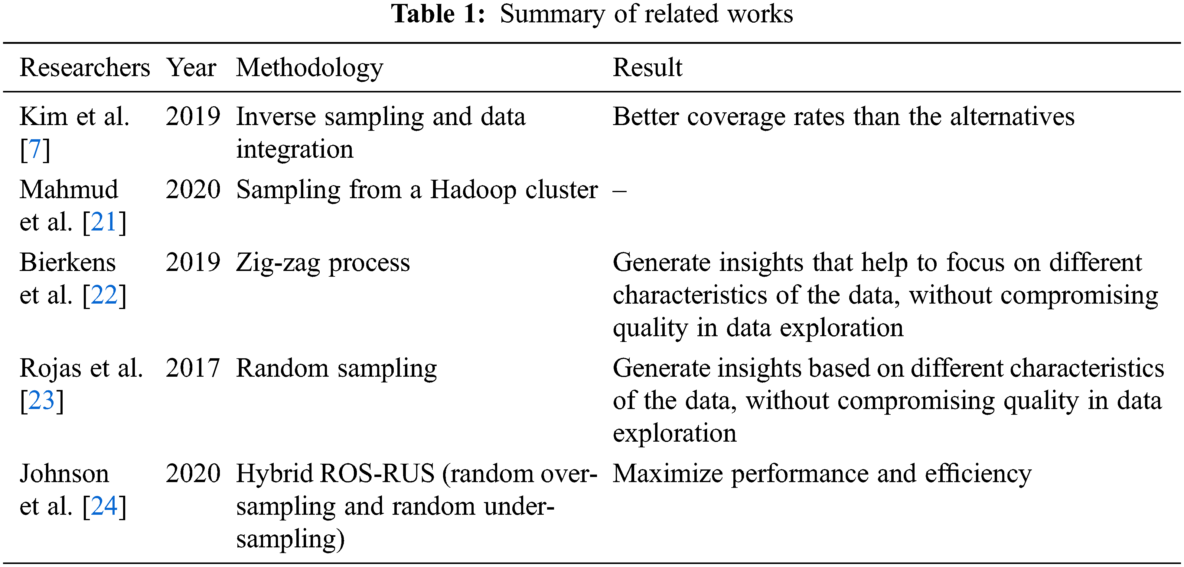
Kim et al. [7] proposed two methods of reducing selection bias associated with big data sampling. The first method uses a version of inverse sampling by incorporating auxiliary information from external sources. The second one integrates data by combining a big data sample with an independent probability sample. Two simulation studies showed that the proposed methods are unbiased and have better coverage rates than their alternatives. In addition, the proposed methods were easy to implement in practice.

Mahmud et al. [21] summarized the available strategies and related work on sampling-based approximations with Hadoop clusters. They suggested that data partitioning and sampling should be considered together to build approximate cluster-computing frameworks that are reliable both computationally and statistically.

Bierkens et al. [22] showed how the zig-zag process can be simulated without discretization errors and give conditions for the process to be ergodic. Most importantly, they introduced a sub-sampling version of the zig-zag process that is an example of an exact approximate scheme. That is, the resulting approximate process still has the posterior as its stationary distribution. Furthermore, if we use a control variate to reduce the variance of our unbiased estimator, then the zig-zag process can be very efficient. After an initial preprocessing step, essentially independent samples from the posterior distribution are obtained at a computational cost that does not depend on the size of the data.

Rojas et al. [23] used a survey to show that random sampling is the only technique commonly used by data scientists to quickly gain insights from a big dataset, despite theoretical and empirical evidence from the active learning community that suggests that there are benefits of using other sampling techniques. Then, to evaluate and demonstrate the benefits of these other sampling techniques, they conducted an online study with 34 data scientists. These scientists performed a data exploration task to support a classification goal using data samples from more than 2 million records of editing data from Wikipedia articles, generated using different sampling techniques. The results demonstrate that, in data exploration, sampling techniques other than random sampling can generate insights based on different characteristics of the data, without compromising quality.

Johnson et al. [24] used three datasets of varying complexity to evaluate data sampling strategies for treating high class imbalance with deep neural networks and big data. The sampling rates were varied to create training distributions with positive class sizes from 0.025% to 90%. The area under the receiver operating characteristics curve was used to compare performance, and thresholding was used to maximize class performance. Random over-sampling (ROS) consistently outperformed under-sampling (RUS) and baseline methods. The majority class was susceptible to misrepresentation when using RUS, and the results suggest that each dataset was uniquely sensitive to imbalance and sample size. The hybrid ROS-RUS maximizes performance and efficiency, and it is our preferred method for treating high imbalance within big data.

These works are summarized in Tab. 1.

Many model methods and techniques have been devised for deep content based prediction. Most perform relatively well but there are still some limitations that hinder the accuracy of the models, so that they are not optimal. Most of these limitations apply to almost all the models, so we will discuss them in general terms. The first limitation is the integrity of the dataset used. Data quality has a very important role in the effectiveness of a model, so if the right dataset is not used then the model’s ability to be trained will be hindered. The second limitation is that in sampling, if there are too many outliers in the sampled data that is to be used for training, then the model will not perform well. Hence, data cleaning and transformation are very important. Finally, the choice of model and the method of adjusting the parameters and hyperparameters also have a role in the effectiveness of the model. If done wrong, the model will not be successful.

2  Categories and Applications of Big Data Analytics

There are four categories of big data analytics. The first category is descriptive analytics, which produces simple descriptions and visualizations that indicate what has transpired in a given period [25]. These are the most recent and sophisticated analytics tools [26]. The second category is diagnostic analytics [27]. Experts can conduct a deep data interrogation to establish why a particular event occurred. The third most common is predictive analytics, which relies on very sophisticated algorithms to predict future events [27]. Finally, prescriptive analytics can identify for an organization the resources it should use or investments it should make to accomplish desired outcomes [28]. To be effective, prescriptive analytics requires very sophisticated machine-learning capacities.

Big data analytics is used for several reasons. First, it can enable business transformation. Generally, managers feel that big data analytics provide significant opportunities for transformation [27]. Additionally, big data analytics can give a company a competitive advantage. It also inspires innovation. Big data analytics can help companies to develop new products that are attractive to its clients. In addition, it can help them discover new possibilities for income generation [27]. Firms using big data analytics are often successful at cutting costs. Moreover, it helps businesses to improve their customer service since they are better able to understand and respond to customers’ views in real time.

Big data analytics can help with national security, as they provide state-of-the-art techniques in the fight against terrorism and crime. There is a wide range of case studies and application scenarios [25]. Big data application is also instrumental in fighting pornography [7,26,27], mainly through “techniques for indexing and retrieval of image and videos by using the extracted text” [28]. Recognizing child pornography is one of the duties of law enforcement agencies, particularly if there has been a crime, allowing child abusers to be quickly apprehended [12]. The NuDetective Forensic Tool helps with the quick identification of child pornography [12]. Images and videos of child pornography are identified using a tactic based on data mining and sampling structures in videotape libraries [29]. Bag-of-visual-features [30] and tag-based image retrieval methods [31] can successfully recognize objects and classify films shared through social media platforms. Filtering social media content can also detect the spread of child pornography [32]. Content filtering is extremely hard, not only because illegal files contain sensitive material, such as pornography, but also because videos are widely spread through social media, inhibiting the application of controlled priori data [33–35].

3  Methodology

To study the influence of sampling techniques on training models, two models were chosen. Since the data consisted of images, models based on a convolutional neural network [36] were considered to be the most suitable [37]. The two models were AlexNet and DenseNet. These with datasets produced by sampling with replacement and reservoir sampling (Fig. 1).

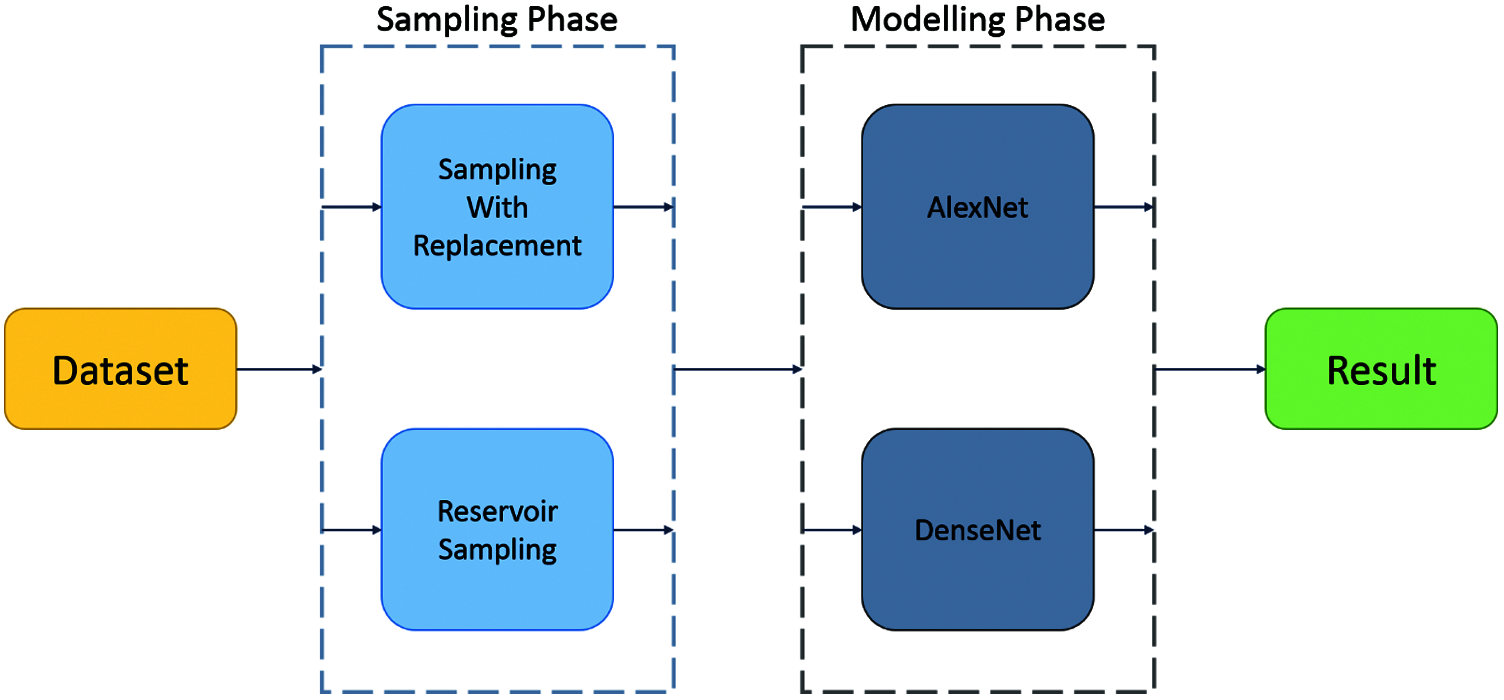
Figure 1: The experimental methodology

3.1 Alexnet

AlexNet was the first convolutional network to used GPUs to boost performance. It was developed by Alex Krizhevsky [36]. As illustrated in Fig. 2, this model has five 2-D convolutional layers, of which three are followed by a max-pooling layer. Each layer is followed by a rectified linear unit (ReLU) [38]. This is followed by an average-pooling layer and a dense layer [39]. There are also two normalization layers, two fully connected layers, and a softmax layer. The pooling layers are used to perform max pooling. The input size is fixed due to the fully connected layers. The input size is 224 × 224 × 3 but with padding it is 227 × 227 × 3. AlexNet overall has 60 million parameters [40]. In this experiment, the AlexNet model used was pre-trained with the ImageNet dataset, and only the parameters of the last linear layer were updated using backpropagation.

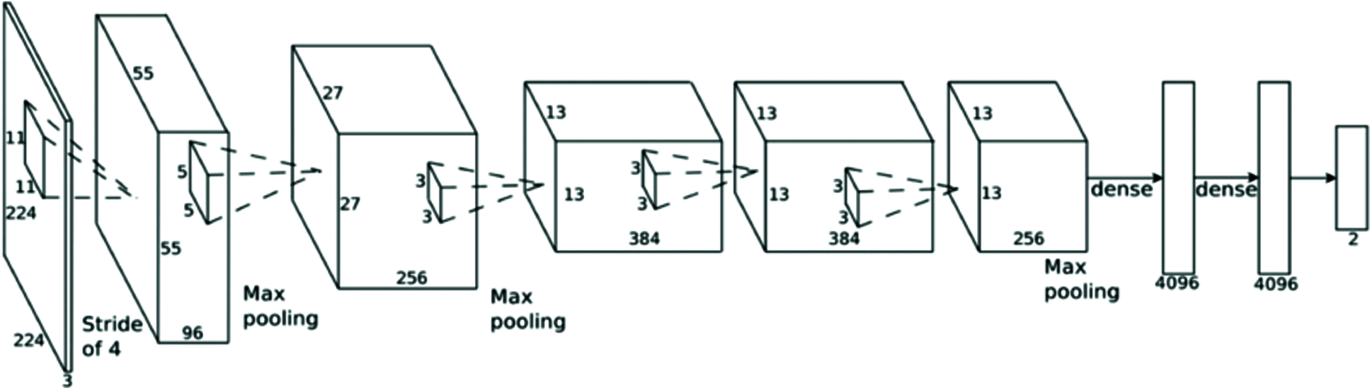
Figure 2: Architecture of AlexNet [40]

AlexNet won the ImageNet Large Scale Visual Recognition Challenge. The model that won the competition was tuned as follows. ReLU was an activation function. Normalization layers were used, which are not common anymore. The batch size was 128. The learning algorithm was SGD Momentum. It used a large amount of data augmentation, such as flipping, jittering, cropping, color normalization, etc. Models were used in ensembles to give the best results.

3.2 Densenet

DenseNet is a type of convolutional neural network that utilizes dense connections between layers through dense blocks (Fig. 3). The DenseNet model was developed by Krizhevsky [41]. A characteristic of this model is the dense blocks, which have multiple layers. Each layer is connected directly to all the subsequent layers in the block. Each layer is basically a composite function of batch normalization [42], followed by a ReLU and a convolution. There are four such dense blocks. Each pair of blocks is separated by a transition layer composed of convolution and pooling functions. The last layer is a linear layer. To preserve the feed-forward nature, each layer has additional inputs from all preceding layers and passes on its feature maps to all subsequent layers [41]. DenseNet was developed specifically to improve the reduced accuracy caused by the vanishing gradient in high-level neural networks. In simpler terms, due to the longer path between the input layer and the output layer, information can vanish before reaching its destination [43–46]. In this experiment, the DenseNet model used was pre-trained with the ImageNet dataset, and only the parameters of the last linear layer were updated using backpropagation.

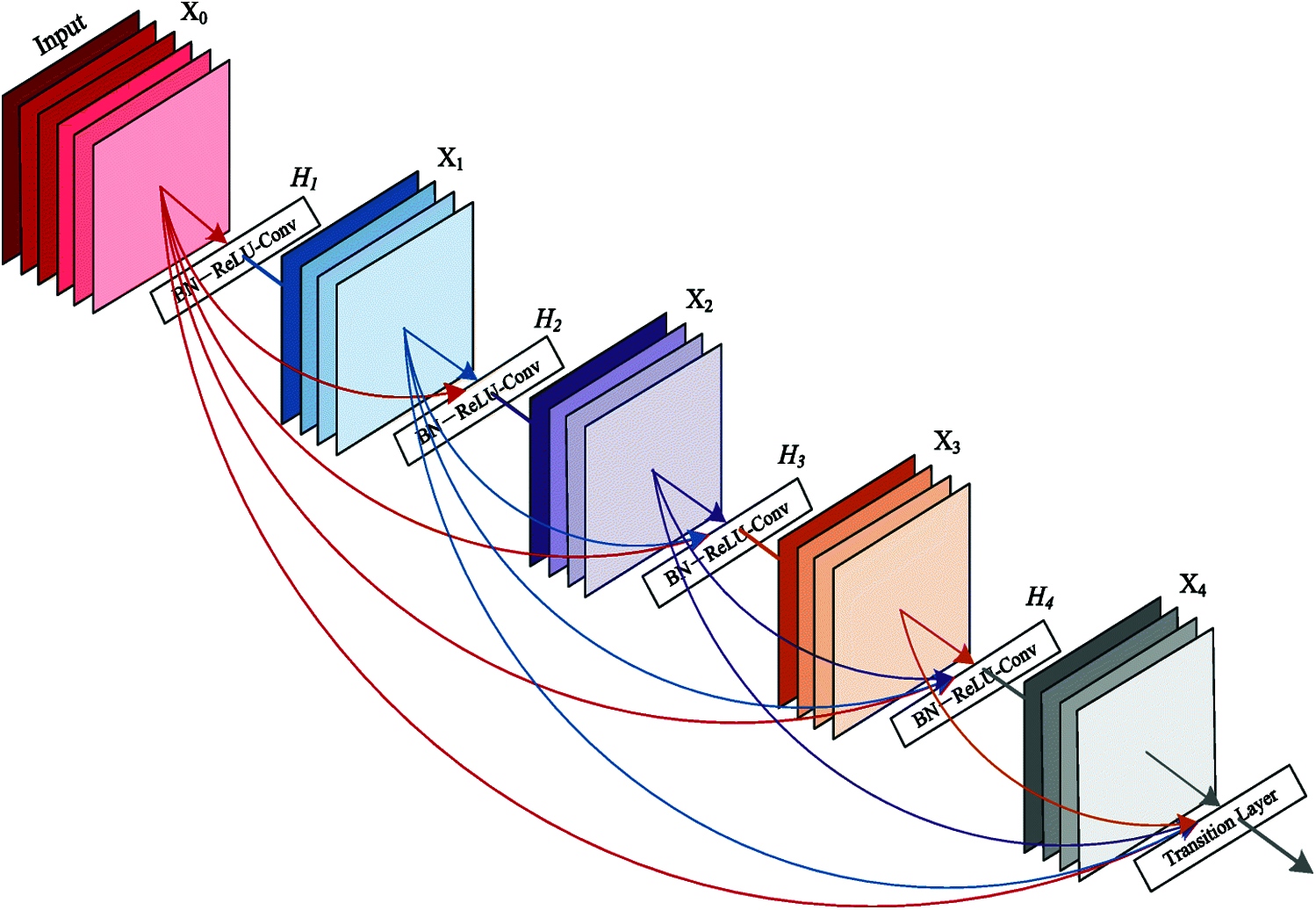
Figure 3: Architecture of DenseNet [41]

4  Experimental Results and Analysis

4.1 Dataset

This paper uses a dataset composed of key images extracted from the NDPI videos [34]. For experimental analysis, the data were divided into three categories: acceptable, flagged as easy, and flagged as hard. The images were then classified. There are two main reasons for choosing these images and image classification. First, in the world of deep learning, image classification is one of the most interesting and researched topics. Second, the dataset is considered to be big, as it has more than 16,000 image frames. Therefore, it is assumed that the data that are processed in this article are big data, and so the results can be extended to other datasets of similar nature.

4.2 Sampling

The experiments done for this study aim to analyze the influence of sampling techniques on the outcome of models. Sampling techniques are important as they could allow deep learning models to achieve comparable results with less data and spend less time on training the model. The two sampling techniques used in this paper are sampling with replacement and reservoir sampling. We reduced the amount of data using random sampling by removing 50% of the instances. The performance and predictability of the trained model were then compared. The sampling was done as follows:

•   In sampling with replacement, an instance is chosen randomly from the dataset. This continues until the number of instances selected is half the number in the complete dataset. However, every time an instance is chosen, it is still available for selection. Thus, the same instance can be sampled multiple times.

•   In reservoir sampling, the samples are chosen without replacement. Thus, each instance can occur at most once in the sampled data. If the complete dataset has n instances and we need k samples, then it can be shown that with the reservoir sampling algorithm [35], each item in the full dataset has the same probability (i.e., k/n) of being chosen for the sampled dataset. We initially select the first k instances of the dataset for our sample. Then we proceed to pick the jth instance (j > k) and decide whether it will be included in the sample (by replacing one of the k selected instances) or rejected, based on a random draw of an integer in the subset 0 to j.

This process of selecting 50% of the data randomly was repeated 10 times. Each sample was then used to develop a deep learning model, using 90% of the data for training and 10% for testing the generated model.

4.3 Evaluation Metric

The models were evaluated using the F-measure, which is mainly used in state-of-the-art applications for similar problems and is good for this type of task too. The F-measure takes into account precision and recall. The F-measure, also known as the F1 score, is calculated as follows:

F1=2⋅Precision×RecallPrecision+Recall (1)

where

Precision=True positiveTrue positive+False positive (2)

and

Recall=True positiveTrue positive+False negative (3)

4.4 Results

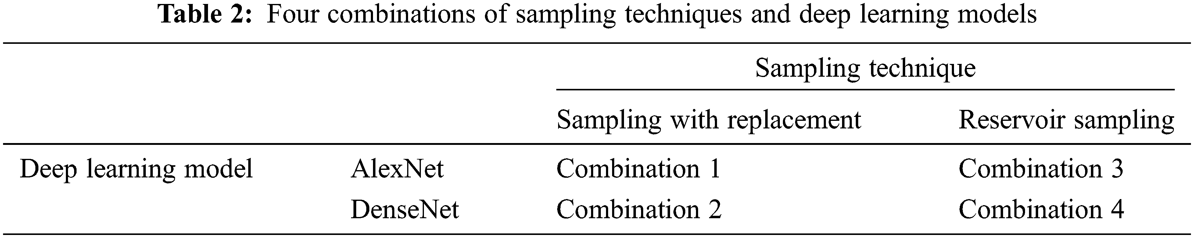
Each model was trained and tested 10 times with each sampling technique. Thus, for each combination of deep learning model and sampling technique, there were 10 experiments. The four combinations are shown in Tab. 2. Thus, 40 experiments were performed for the study. As a baseline, each model was first trained with all the instances from the complete dataset. This is produced a set of base results, which was used to compare the results from experiments performed with 50% of the complete dataset.

As we can see in Fig. 4, the F-measure of the experiments with sampling with replacement is better than that for the base model, although only 50% of the data were used for training the base model. The F-measure of the base model is 0.807, while the very first experiment outperforms this, getting 0.883. The second experiment has an even better score of 0.894. The scores for the 3rd, 4th, 5th, 6th, 7th, 8th, 9th, and 10th experiments are 0.878, 0.884, 0.889, 0.898, 0.884, 0.878, 0.884, and 0.880, respectively. Thus, we can see that in every experiment, the model has a better F-measure than the base model, despite using only half the data for training. The average F-measure of the experiments is 0.885 with a standard deviation of 0.007. Thus, AlexNet models trained with the sampling with replacement technique were better by 7.82% than the model trained with the complete dataset.

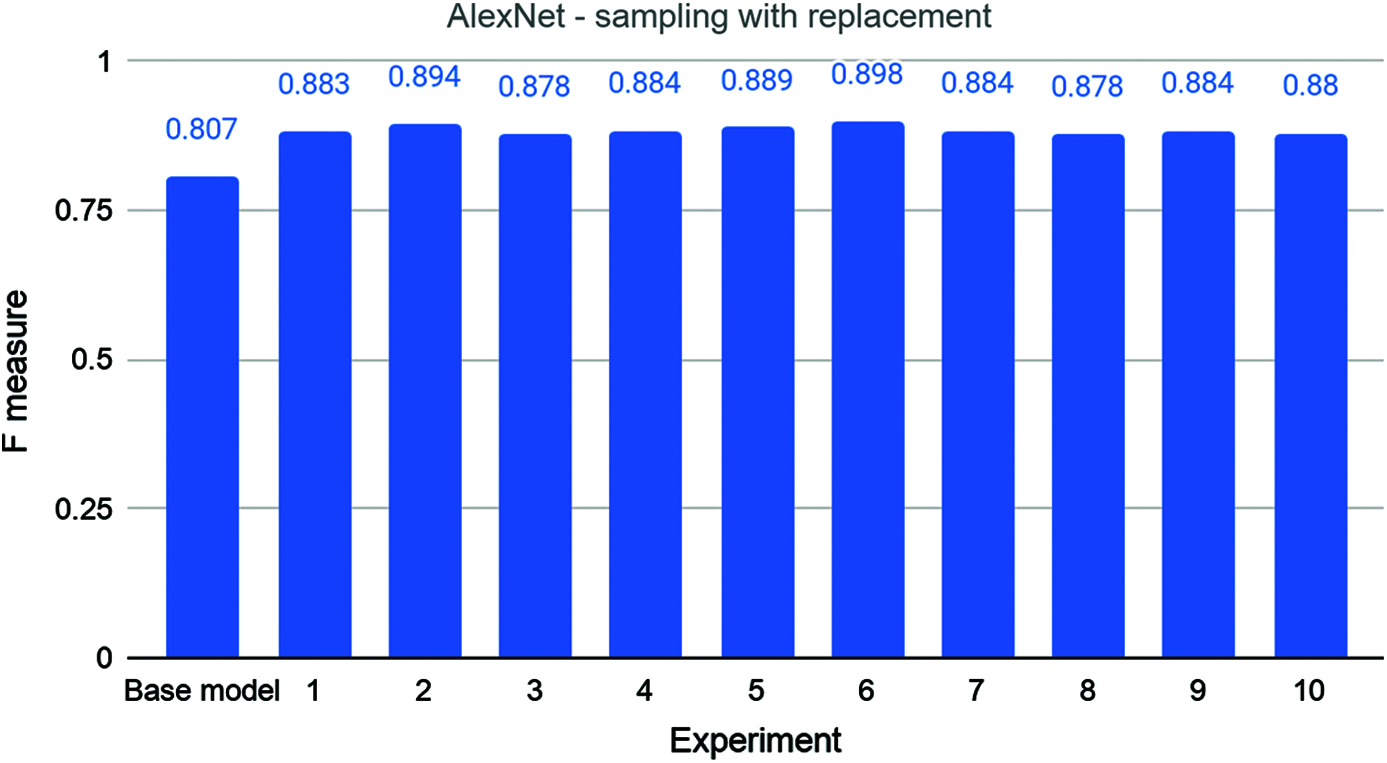
Figure 4: The base and ten rounds of experiments for combination 1

In Fig. 5, we can see the results of experiments conducted with reservoir sampling and the AlexNet model. The base model has an F-measure of 0.807 when trained with the complete dataset, as we saw earlier. The F-measure of the experiments with reservoir sampling is better than that for the base model. The first experiment, with an F-measure of 0.839, outperforms the base model. The second experiment has an even better score of 0.859. The scores of the 3rd, 4th, 5th, 6th, 7th, 8th, 9th, and 10th experiments are 0.853, 0.869, 0.852, 0.866, 0.852, 0.863, 0.842, and 0.850, respectively. Thus, we can see again that in every experiment, the model has a better F-measure than the base model. The average F-measure of the experiments is 0.855 with a standard deviation of 0.010. Thus, AlexNet models trained with reservoir sampling technique were better by 4.75% than the model trained with the complete dataset.

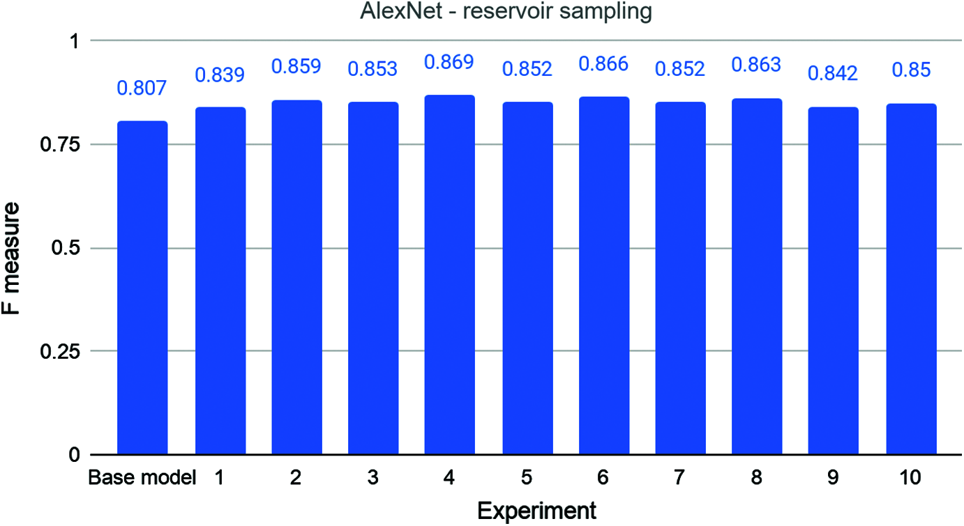
Figure 5: The base and ten rounds of experiments for combination 3

Fig. 6 shows the results of experiments where the DenseNet model was trained using 50% of the data randomly sampled with replacement. The base model has an F-measure of 0.808 when trained with the complete dataset. This graph has a very interesting trend. The first experiment has a lower F-measure of 0.805 than the base model, which is marginally lower. The second and third experiments have even lower scores of 0.782 and 0.780. Although the 4th, 5th, 6th, and 7th experiments did better with F-measures of 0.800, 0.85, 0.805, and 0.801, respectively, these values are still lower than that of the base model. The 8th, 9th, and 10th experiments, however, have an F-measure higher than that of the base model. The scores are 0.812, 0.816, and 0.811. The average F-measure of the experiments is 0.802 with a standard deviation of 0.012. Since the difference between the average score and score of the base model is less than even 1%, it is hard to draw a strong conclusion.

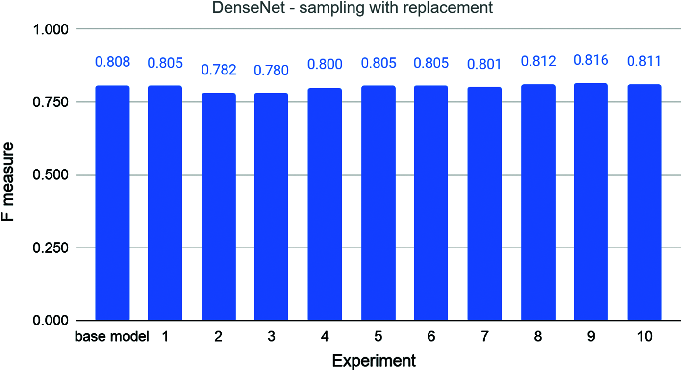
Figure 6: The base and ten rounds of experiments for combination 2

Fig. 7 gives the results of experiments where the DenseNet model was trained using 50% of the data from reservoir sampling. When trained with the complete dataset, the base model has an F-measure of 0.808, as we saw earlier. Again, graph has an interesting trend. The 2nd, 3rd, 4th, 7th, and 10th experiments have F-measures of 0.814, 0.823, 0.811, 0.822, and 0.824, which are all better than that of the base model. The 6th experiment and the base model have the same F-measure. The 1st, 5th, and 9th experiments, in contrast, have scores of 0.802, 0.799, and 0.801, which are all less than that of the base model. The average score is 0.811 with a standard deviation of 0.009. Though this is marginally better than the score of the base model, the difference is less than 1% and strong conclusions cannot be drawn.

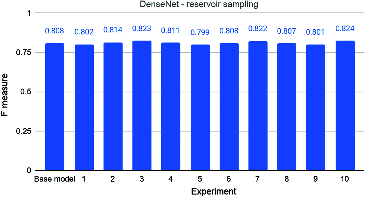
Figure 7: The base and ten rounds of experiments for combination 4

As we can see from the results in Tab. 3, although both sampling techniques give better results on average for the AlexNet model, the same cannot be said for the DenseNet model.

5  Discussion and Conclusions

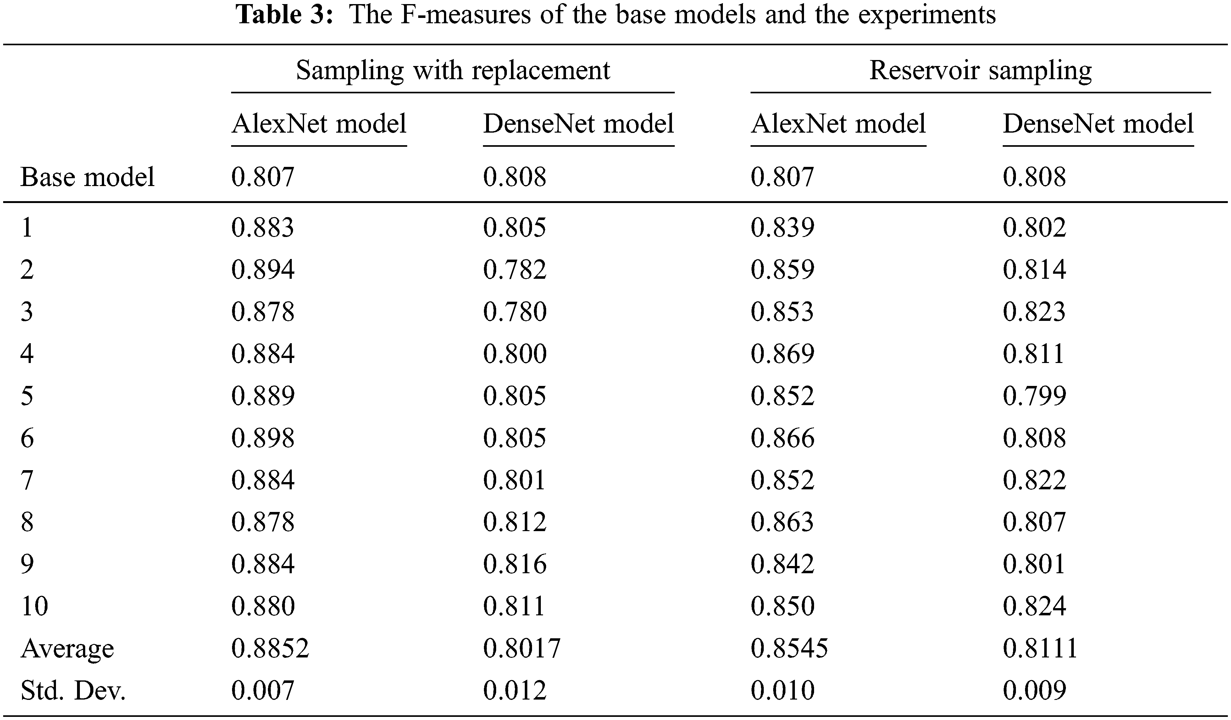
The first experiment conducted was the base case, which used the whole dataset for training and validation, so it was used to compare and test the sampling techniques. AlexNet had an F-measure of 0.807 in the base test. With sampling with replacement, the value was as low as 0.878 and as high as 0.898 with an average of 0.885. These results are excellent compared to the base experiment. With reservoir sampling, the lowest F-measure was 0.839 and the highest was 0.861 with an average of 0.855. These results are also good compared with those for the base experiment. In contrast, with DenseNet, the base experiment has a slightly higher F-measure than the base AlexNet, with a score of 0.808. When sampling with replacement using DenseNet, the lowest score was 0.780 and the highest was 0.816 with an average of 0.802. With reservoir sampling, the lowest score was 0.799 and the highest was 0.824 with an average of 0.811. On average, both techniques with DenseNet are better than the base experiment but not as effective as the AlexNet model.

From the results, it can be seen that the AlexNet model was more accurate by 7.82% and 4.75% for sampling with replacement and reservoir sampling, respectively. However, the DenseNet model did not do as well because its accuracy was very close to that of the base model, with a difference of less than 1% for both sampling with replacement and reservoir sampling. For both models, this research shows that to save the time and cost of analysis and model training, sampling is very useful. Even though not all the data are used, sampling results in the same if not better accuracy than when the original dataset is used.

None of the recent works reported in the literature review used either sampling with replacement or reservoir sampling, both of which gave better results. Some used random sampling, which is less effective compared to other sampling techniques.

There is an endless stream of big data, about 2.5 quintillion bytes every day, from a vast pool of sources such as social media, the internet of things, the cloud, and other databases, just to mention a few. Even though a large amount of data is required for analysis and for deep neural networks to be effectively trained, having too much data is a problem. Although effective results can be obtained with a dataset containing 10,000 items, 10 million is just too many. The time it would take to train a model and analyze this cumbersome amount of data is too long. This research aimed to demonstrate the effectiveness of using only a portion of the data.

The dataset in this research was randomly sampled so that only 50% was used. As there were two deep leaning models (AlexNet and DenseNet) and two sampling techniques (sampling with replacement and reservoir sampling), there were four test combinations. After training, the results were compared to the base models trained on the whole dataset. It was found that the sampled datasets produced the same or higher accuracy during testing. The high accuracy we obtained from the sampled datasets indicates that when analyzing and training deep neural models, it is better to sample the data if there are too much, since it is relatively less time-consuming and achieves effective results.

Acknowledgement: The researchers would like to thank the Deanship of Scientific Research, Qassim University for funding the publication of this project.

Funding Statement: The authors received no specific funding for this study.

Conflicts of Interest: The authors declare that they have no conflicts of interest to report regarding the present study.

References

 1.  S. Madden, “From databases to big data,” IEEE Internet Computing, vol. 16, no. 3, pp. 4–6, 2012. [Google Scholar]

 2.  W. Albattah, R. Khan and K. Khan, “Attributes reduction in big data,” Applied Sciences, vol. 10, no. 14, pp. 4901–4910, 2020. [Google Scholar]

 3.  C. W. Tsai, C. F. Lai, H. C. Chao and A. V. Vasilakos, “Big data analytics: A survey,” Journal of Big Data, vol. 2, no. 1, pp. 1–32, 2015. [Google Scholar]

 4.  J. Zakir, T. Seymour and K. Berg, “Big data analytics,” Issues in Information Systems, vol. 16, no. 2, pp. 81–90, 2015. [Google Scholar]

 5.  G. Bello-Orgaz, J. J. Jung and D. Camacho, “Social big data: Recent achievements and new challenges,” Information Fusion, vol. 28, pp. 45–59, 2016. [Google Scholar]

 6.  R. Clarke, “Big data, big risks,” Information Systems Journal, vol. 26, no. 1, pp. 77–90, 2016. [Google Scholar]

 7.  J. K. Kim and Z. Wang, “Sampling techniques for big data analysis,” International Statistical Review, vol. 87, no. 1, pp. 177–191, 2019. [Google Scholar]

 8.  K. Engemann, B. Enquist, B. Sandel, B. Boyle, P. Jørgensen et al., “Limited sampling hampers ‘big data’ estimation of species richness in a tropical biodiversity hotspot,” Ecology and Evolution, vol. 5, no. 3, pp. 807–820, 2015. [Google Scholar]

 9.  J. Zhao, J. Sun, Y. Zhai, Y. Ding, C. Wu et al., “A novel clustering-based sampling approach for minimum sample set in big data environment,” International Journal of Pattern Recognition and Artificial Intelligence, vol. 32, no. 2, pp. 1850003, 2017. [Google Scholar]

10. S. Liu, R. She and P. Fan, “How many samples required in big data collection: A differential message importance measure,” arXiv preprint, arXiv:1801.04063, 2018. [Google Scholar]

11. A. L’Heureux, K. Grolinger, H. F. Elyamany and M. A. M. Capretz, “Machine learning with big data: Challenges and approaches,” IEEE Access, vol. 5, pp. 7776–7797, 2017. [Google Scholar]

12. P. M. da Silva Eleuterio and M. de Castro Polastro, “An adaptive sampling strategy for automatic detection of child pornographic videos,” in 7th Int. Conf. on Forensic Computer Science, Brasilia, Brazil, pp. 12–19, 2012. [Google Scholar]

13. ACM Digital Library. Proc. of the 5th Annual ACM Workshop on Computational Learning Theory, Pittsburgh, PA, USA, 1992. [Google Scholar]

14. L. Zhou, S. Pan, J. Wang and A. V. Vasilakos, “Machine learning on big data: Opportunities and challenges,” Neurocomputing, vol. 237, no. 1, pp. 350–361, 2017. [Google Scholar]

15. K. Kowsari, D. E. Brown, M. Heidarysafa, K. J. Meimandi, M. S. Gerber et al., “HDLTex: Hierarchical deep learning for text classification,” in 16th IEEE Int. Conf. on Machine Learning and Applications (ICMLA), Cancun, Mexico, pp. 364–371, 2017. [Google Scholar]

16. C. Farabet, C. Couprie, L. Najman and Y. LeCun, “Learning hierarchical features for scene labeling,” IEEE Transactions on Pattern Analysis and Machine Intelligence, vol. 35, no. 8, pp. 1915–1929, 2013. [Google Scholar]

17. M. M. Najafabadi, F. Villanustre, T. M. Khoshgoftaar, N. Seliya, R. Wald et al., “Deep learning applications and challenges in big data analytics,” Journal of Big Data, vol. 2, no. 1, pp. 1–21, 2015. [Google Scholar]

18. S. Tong and D. Koller, “Support vector machine active learning with applications to text classification,” Journal of Machine Learning Research, vol. 2, pp. 45–66, 2001. [Google Scholar]

19. J. F. Torres, A. Galicia, A. Troncoso and F. Martínez-Álvarez, “A scalable approach based on deep learning for big data time series forecasting,” Integrated Computer-Aided Engineering, vol. 25, no. 4, pp. 335–348, 2018. [Google Scholar]

20. C. Jansohn, A. Ulges and T. M. Breuel, “Detecting pornographic video content by combining image features with motion information,” in 17th ACM Int. Conf. on Multimedia (MM ‘09), Beijing, China, pp. 601–604, 2019. [Google Scholar]

21. M. S. Mahmud, J. Huang, S. Salloum, T. Emara and K. Sadatdiynov, “A survey of data partitioning and sampling methods to support big data analysis,” Big Data Mining and Analytics, vol. 3, no. 2, pp. 85–101, 2020. [Google Scholar]

22. J. Bierkens, P. Fearnhead and G. Roberts, “The zig-zag process and super-efficient sampling for Bayesian analysis of big data,” Annals of Statistics, vol. 47, no. 3, pp. 1288–1320, 2019. [Google Scholar]

23. A. J. Rojas, M. B. Kery, S. Rosenthal and A. Day, “Sampling techniques to improve big data exploration,” in 2017 IEEE 7th Symp. on Large Data Analysis and Visualization (LDAV), Phoenix, AZ, USA, pp. 26–35, 2017. [Google Scholar]

24. J. M. Johnson and T. M. Khoshgoftaar, “The effects of data sampling with deep learning and highly imbalanced big data,” Information Systems Frontiers, vol. 22, no. 5, pp. 1113–1131, 2020. [Google Scholar]

25. A. Liaw and M. Wiener, “Classification and regression by randomForest,” R News, vol. 2, no. 3, pp. 18–22, 2012. [Google Scholar]

26. M. Hilbert, “Big data for development: A review of promises and challenges,” Development Policy Review, vol. 34, no. 1, pp. 135–174, 2016. [Google Scholar]

27. D. Sullivan, “Introduction to big data security analytics in the enterprise,” Tech Target, pp. 1–401, 2015. [Google Scholar]

28. J. Bierkens, P. Fearnhead and G. Robert, “The zig-zag process and super-efficient sampling for Bayesian analysis of big data,” The Annals of Statistics, vol. 47, no. 3, pp. 1288–1320, 2019. [Google Scholar]

29. B. Akhgar, G. B. Saathoff, H. R. Arabnia, R. Hill, A. Staniforth et al., “Application of big data for national security: A practitioner’s guide to emerging technologies,” Butterworth-Heinemann, 2015. [Google Scholar]

30. N. Agarwal, “Blocking objectionable web content by leveraging multiple information sources abstract,” ACM SIGKDD Explorations Newsletter, vol. 8, no. 1, pp. 17–26, 2006. [Google Scholar]

31. H. Lee, S. Lee and T. Nam “Implementation of high-performance objectionable video classification system,” in 8th Int. Conf. Advanced Communication Technology, Phoenix Park, South Korea, 2006. [Google Scholar]

32. A. N. Bhute and B. B. Meshram, “Text based approach for indexing and retrieval of image and video: A review,” Advances in Vision Computing, vol. 1, no. 1, pp. 701–712, 2014. [Google Scholar]

33. J. -H. Wang, H. -C. Chang, M. -J. Lee and Y. -M. Shaw, “Classifying peer-to-peer file transfers for objectionable content filtering using a web-based approach,” IEEE Intelligent Systems, vol. 17, pp. 48–57, 2002. [Google Scholar]

34. A. P. B. Lopes, S. E. F. de Avila, A. N. A. Peixoto, R. S. Oliveira, M. d. M. Coelho et al., “Nude detection in video using bag-of-visual-features,” in XXII Brazilian Symp. on Computer Graphics and Image Processing, Rio de Janeiro, Brazil, pp. 224–231, 2009. [Google Scholar]

35. S. Badghaiya and A. Bharve, “Image classification using tag and segmentation based retrieval,” International Journal of Computer Applications, vol. 103, no. 15, pp. 20–23, 2014. [Google Scholar]

36. W. Albattah and S. Albahli, “Content-based prediction: Big data sampling perspective,” International Journal of Engineering & Technology, vol. 8, no. 4, pp. 627–635, 2019. [Google Scholar]

37. E. Valle, S. de Avila, A. de Luz Jr., F. de Souza, M. Coelho et al., “Content-based filtering for video sharing social networks,” arXiv preprint, arXiv:1101.2427, 2015. [Google Scholar]

38. S. Avila, N. Thome, M. Cord, E. Valle and A. d. A. Araújo, “Pooling in image representation: The visual codeword point of view,” Computer Vision and Image Understanding, vol. 117, no. 5, pp. 453–465, 2013. [Google Scholar]

39. N. Alrobah and S. Albahli, “A hybrid deep model for recognizing arabic handwritten characters,” IEEE Access, vol. 9, pp. 87058–87069, 2021. [Google Scholar]

40. J. S. Vitter, “Random sampling with a reservoir,” ACM Transactions on Mathematical Software, vol. 11, no. 1, pp. 37–57, 1985. [Google Scholar]

41. A. Krizhevsky, “One weird trick for parallelizing convolutional neural networks,” arXiv preprint, arXiv:1404.5997, 2014. [Google Scholar]

42. M. M. Krishna, M. Neelima, M. Harshali and M. V. G. Rao, “Image classification using deep learning,” International Journal of Engineering & Technology, vol. 7, no. 2.7, pp. 614–617, 2018. [Google Scholar]

43. X. Glorot, A. Bordes and Y. Bengio, “Deep sparse rectifier neural networks,” in 14th Int. Conf. on Artificial Intelligence and Statistics, Fort Lauderdale, FL, USA, pp. 315–323, 2011. [Google Scholar]

44. S. Albahli, N. Ayub and M. Shiraz, “Coronavirus disease (COVID-19) detection using X-ray images and enhanced denseNet,” Applied Soft Computing, vol. 110, pp. 107645, 2021. [Google Scholar]

45. S. Ioffe and C. Szegedy, “Batch normalization: Accelerating deep network training by reducing internal covariate shift,” arXiv preprint, arXiv:1502.03167, 2015. [Google Scholar]

46. Great Learning Team, “Alexnet: The first CNN to win image Net,” June, 2020. https://www.mygreatlearning.com/blog/alexnet-the-first-cnn-to-win-image-net/. [Google Scholar]