Stable Computer Method for Solving Initial Value Problems with Engineering Applications

1  Introduction

Differential equations include ordinary and partial derivatives. Initial value problems (IVPs) are formed by utilizing ordinary differential equations and initial conditions to provide the value of an unknown function at a specific place in the domain. Differential equations are commonly used in physics, chemistry, biology, and economics, as well as in many physical problems in science and engineering.

Numerous analytical techniques are available to solve differential equations. Analytical techniques [1,2], however, are sometimes unable are very difficult to provide closed form solutions of linear or nonlinear differential equations. Therefore, numerical methods are frequently used to solve highly nonlinear and linear differential equations [3]. Numerical techniques are important tools for quickly solving difficult problems using computer programming. To solve IVPs, engineers and researchers from a variety of disciplines [4–7] needed numerical schemes that were more efficient, stable, and had a larger region of convergence than other techniques that already existed and had the same order of convergence.

Numerous numerical algorithms for solving ordinary differential equations (ODEs) with initial value problems have been developed by many researchers. Many authors have attempted to solve initial value problems with great accuracy and speed up using various methods such as Euler’s method, Heun’s method, and others (see e.g., [8–12]). Euler’s method calculates the slope of the function over the interval by using the line, tangent to the function at the beginning of the interval. In comparison, Heun’s method considers tangent lines to the solution curve at both ends of the interval. Some have attempted to improve these precision approaches, while others have enhanced them for greater accuracy, stability, and consistency [13,14]. Some changes have been made to numerical algorithms from time to time to improve the performance based on our needs.

The main aim of this study was to construct a novel numerical technique for solving both linear and nonlinear initial value problems. Using consistency and stability analyses, we illustrate that the region of stability of our recently proposed numerical techniques is wider than the methods currently available in the literature. Compared with other techniques already in use, our newly developed method is more reliable, consistent, and efficient.

2  Proposed Method’s Methodology Approach

Consider the following first-order differential equation with an initial value problem:

dydx=f(x,y);y(x0)=y0. (1)

The most well-known and simple approach for solving Eq. (1) is the explicit Euler equation’ with step length h, which is given by

yn+1p=yn+hf(xn,yn). (2)

The explicit Euler method [15] approximates the derivative of y0 at x=xn using forward difference. Heun’s method has a slope that is the average of the slope of the tangents to the integral curve at the endpoint of the interval, given by

yn+1c=yn+h2[f(xn,yn)+f(xn+1,yn+1p)]. (3)

In [16], using Euler’s method as a predictor, a second stage of the second-order method (MRK2M) based on the harmonic mean is presented as:

{yn+1=yn+h2(k12+k22k1+k2),k1=f(xn,yn),k2=f(xn+1,ypn+1). (4)

Here, we propose modified version (MMRK2M) of Eq. (4) as:

{yn+1=yn+h(k12+k32k1+k3),k1=f(xn,yn),k2=f(xn+1,yn+1p),k3=f(xn+h,yn+h(k1+k22)). (5)

3  Analysis of the Proposed Method’s Stability

Dahlquist’s test problem [17] can be used to analyze the stability of the proposed scheme.

dydx=λyn;y(x0)=y0,λ∈C. (6)

Eq. (5) can also be written as:

yn+1=yn+h((f(xn,yn))2+(f(xn+h,yn+h(f(xn,yn)+f(xn+1,yn+1p)2)))2f(xn,yn)+f(xn+h,yn+h(f(xn,yn)+f(xn+1,yn+1p)2))). (7)

To test the stability of the suggested approach, substitute Eq. (6) with Eq. (5), and we have

yn+1=yn+h((f(xn,yn))2+(f(xn+h,yn+h(f(xn,yn)+f(xn+1,yn+1p)2)))2f(xn,yn)+f(xn+h,yn+h(f(xn,yn)+f(xn+1,yn+1p)2))), (8)

yn+1=yn+h2λ2yn2+(hλyn+h2λ2yn+12h3λ3yn)2hλyn+hλyn+12h3λ3yn, (9)

yn+1=(1+h2λ2+(hλ+h2λ2+12h3λ3)2hλ+hλ+12h3λ3)yn. (10)

Putting z=hλ in Eq. (10), we have

Q(z)=yn+1yn=1+z2+(z+z2+12z3)2z+z2+12z3, (11)

The stability region of numerical systems is depicted in Figs. 1 and 2. The stability polynomial is given by

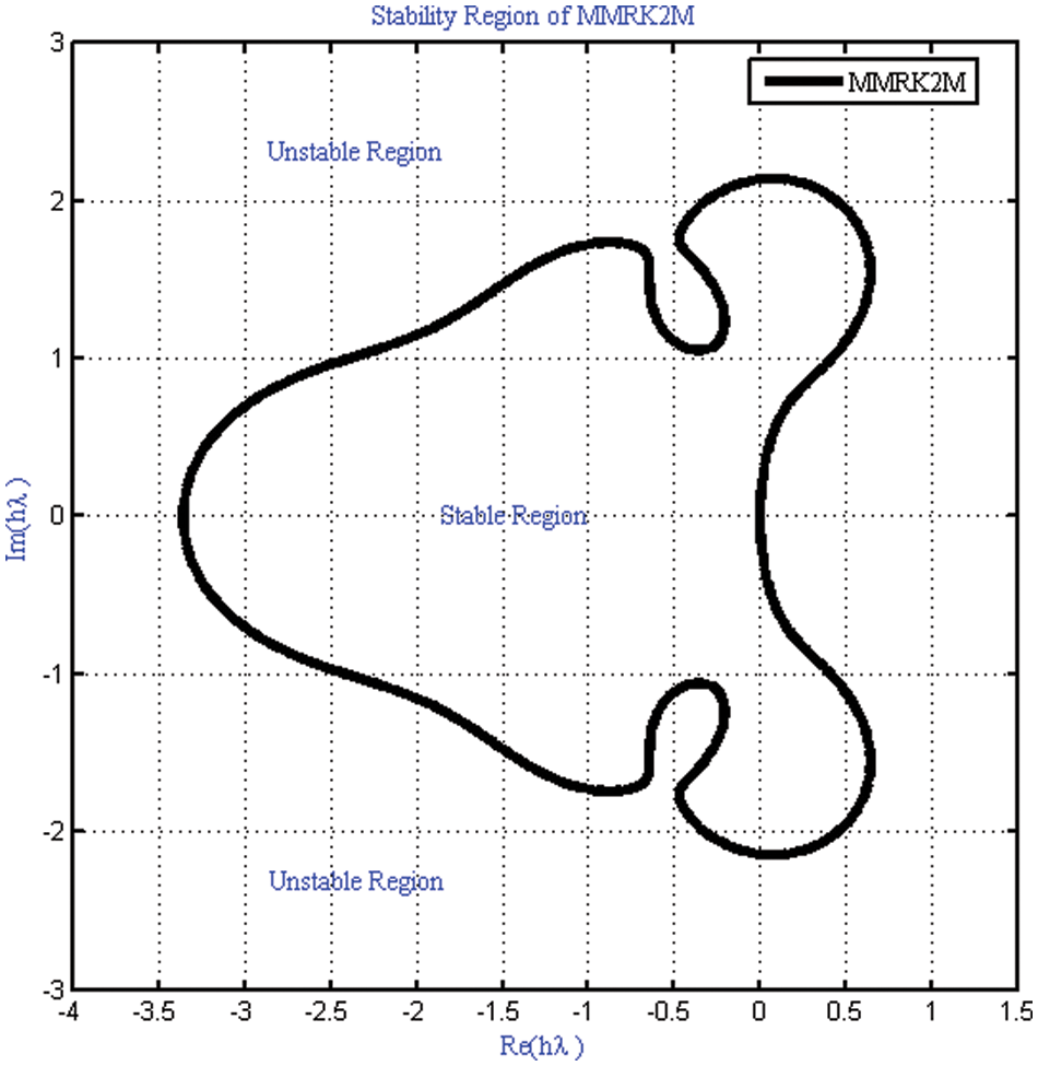
Figure 1: Stability region of MMRK2M is represented by white color where shading region shows instability region of the proposed method

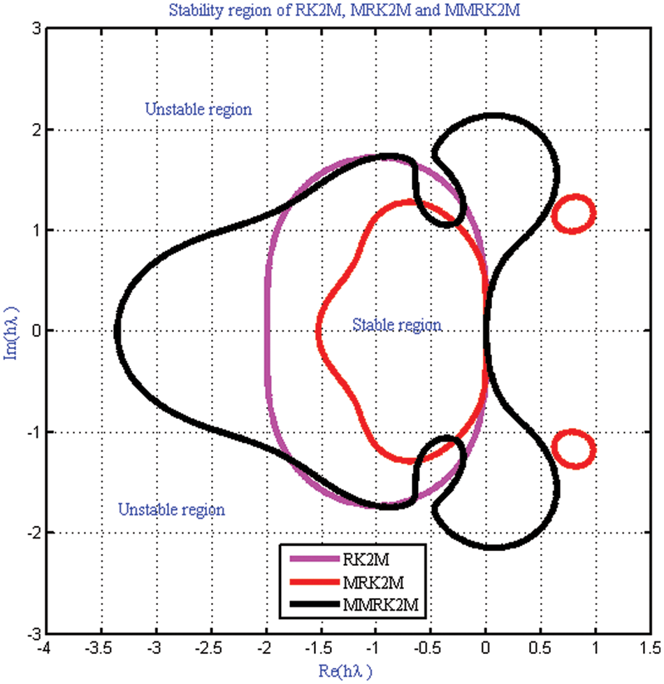
Figure 2: Comparison of the stability region of the proposed method MMRK2M (Black color) with MRK2 (Red color) and MRK2M (Cyan color) respectively

|Q(z)|=|yn+1yn|=|1+z2+(z+z2+12z3)2z+z2+12z3|≤1. (12)

4  Consistency

To verify the consistency [17,18] of the proposed method, Eq. (5) can be written as:

yn+1=yn+hϑ(xn,yn,h), (13)

and numerical scheme will be consistent if

limh→0⁡ϑ(xn,yn,h)=f(xn,yn). (14)

In this case, we used equation Eq. (13) to determine the consistency of the proposed technique as follows:

limh→0⁡ϑ(xn,yn,h)=limh→0⁡((f(xn,yn))2+(f(xn+h,yn+h(f(xn,yn)+f(xn+1,yn+1p)2)))2f(xn,yn)+f(xn+h,yn+h(f(xn,yn)+f(xn+1,yn+1p)2))),=f(xn,yn). (15)

Thus, proposed method is consistent.

5  Local Truncation Error

The local truncation error of a numerical technique is an estimate of the error introduced in a single iteration of the method, assuming that everything provided in the method is exact.

The Taylor series expansion of y(xn+1) is given by:

y(xn+1)=y(xn+h)=y(xn)+hy′(xn)+h22!y′′(xn)+h33!y′′′(xn)+O(h4), (16)

y(xn+1)=y(xn)+hf(xn,yn)+h22!(∂f(xn,yn)∂x+f(xn,yn)∂f(xn,yn)∂y)+... (17)

The Taylor series expansion of

k1=f(xn,yn), (18)

k2=k2=f(xn+h,yn+hf(xn,yn)),=f(xn,yn)+h(∂f(xn,yn)∂x+f(xn,yn)∂f(xn,yn)∂y)+h22!(∂2f(xn,yn)∂x2+2f(xn,yn)∂2f(xn,yn)∂x∂y+(f(xn,yn))2∂2f(xn,yn)∂2y)+O(h3), (19)

k1+k22=f(xn,yn)+h2(∂f(xn,yn)∂x+f(xn,yn)∂f(xn,yn)∂y)+O(h2), (20)

k3=f(xn,yn)+h(∂f(xn,yn)∂x+f(xn,yn)∂f(xn,yn)∂y)+O(h2), (21)

yn+1=yn+h((f(xn,yn))2+(f(xn,yn)+h(∂f(xn,yn)∂x+f(xn,yn)∂f(xn,yn)∂y)+O(h2))2f(xn,yn)+f(xn,yn)+h(∂f(xn,yn)∂x+f(xn,yn)∂f(xn,yn)∂y)+O(h2)), (22)

yn+1=yn+hf(xn,Yn)+h22!(∂f(xn,yn)∂x+f(xn,yn)∂f(xn,yn)∂y)+O(h3). (23)

As a result of subtracting Eq. (23) or Eq. (22) from Eq. (17), the proposed numerical technique has a local truncation error of order O(h3) ; hence, the order of the proposed method is 2.

6  Numerical Outcomes

We execute the following iterative methods

1.    Newly constructed method MMRK2M

2.    Modified Euler method MRK2

3.    Ram et al. method MRK2M

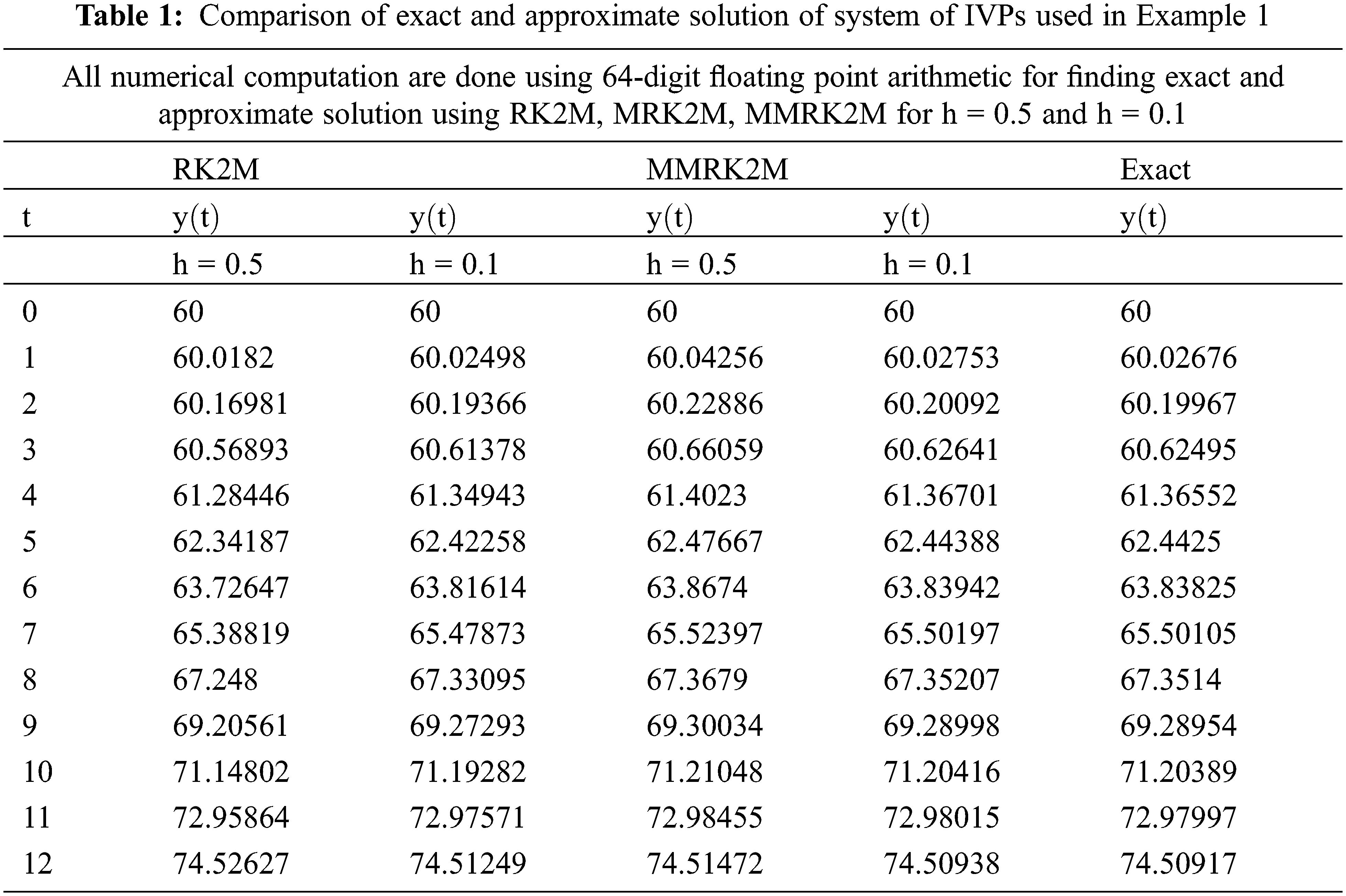
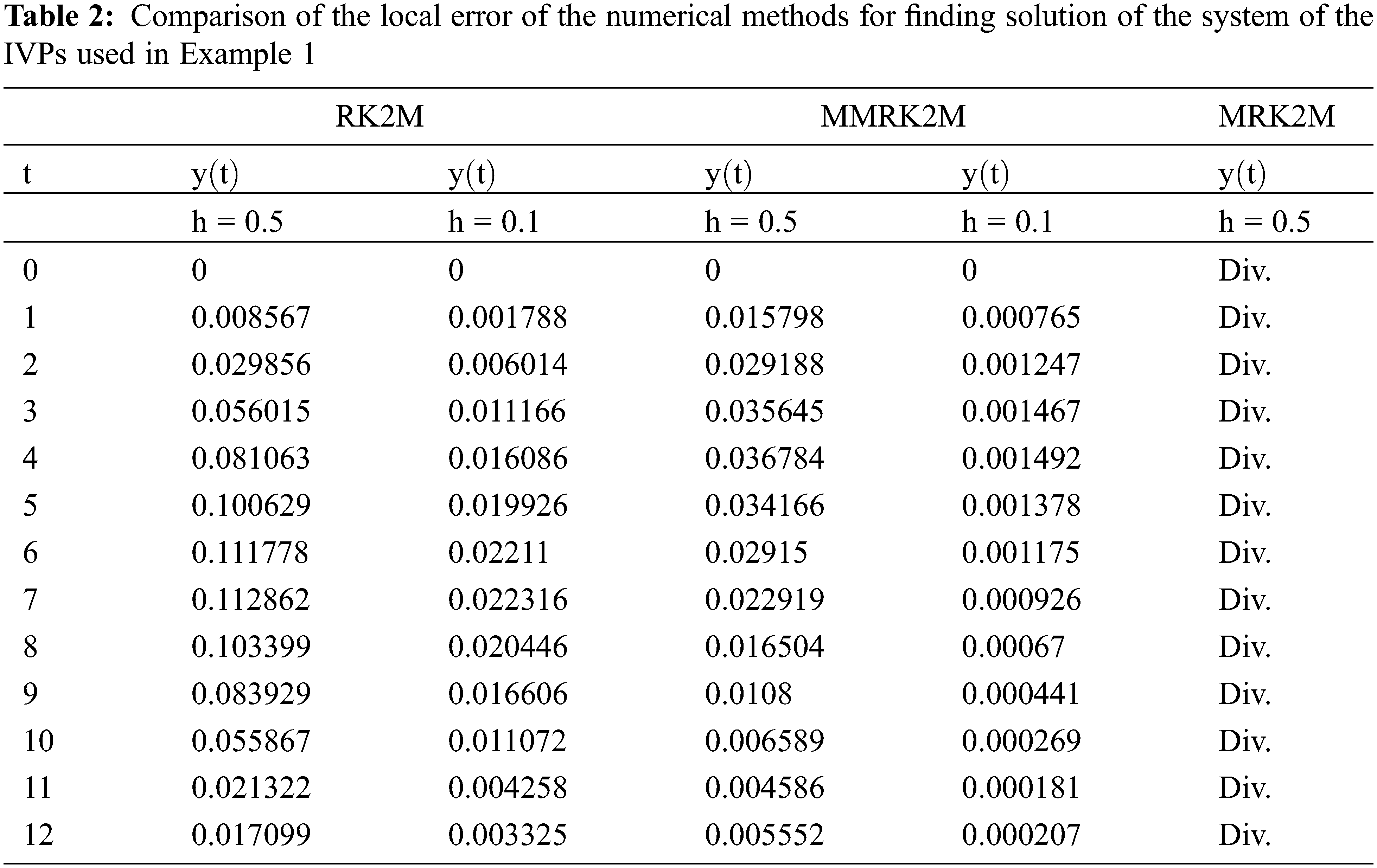
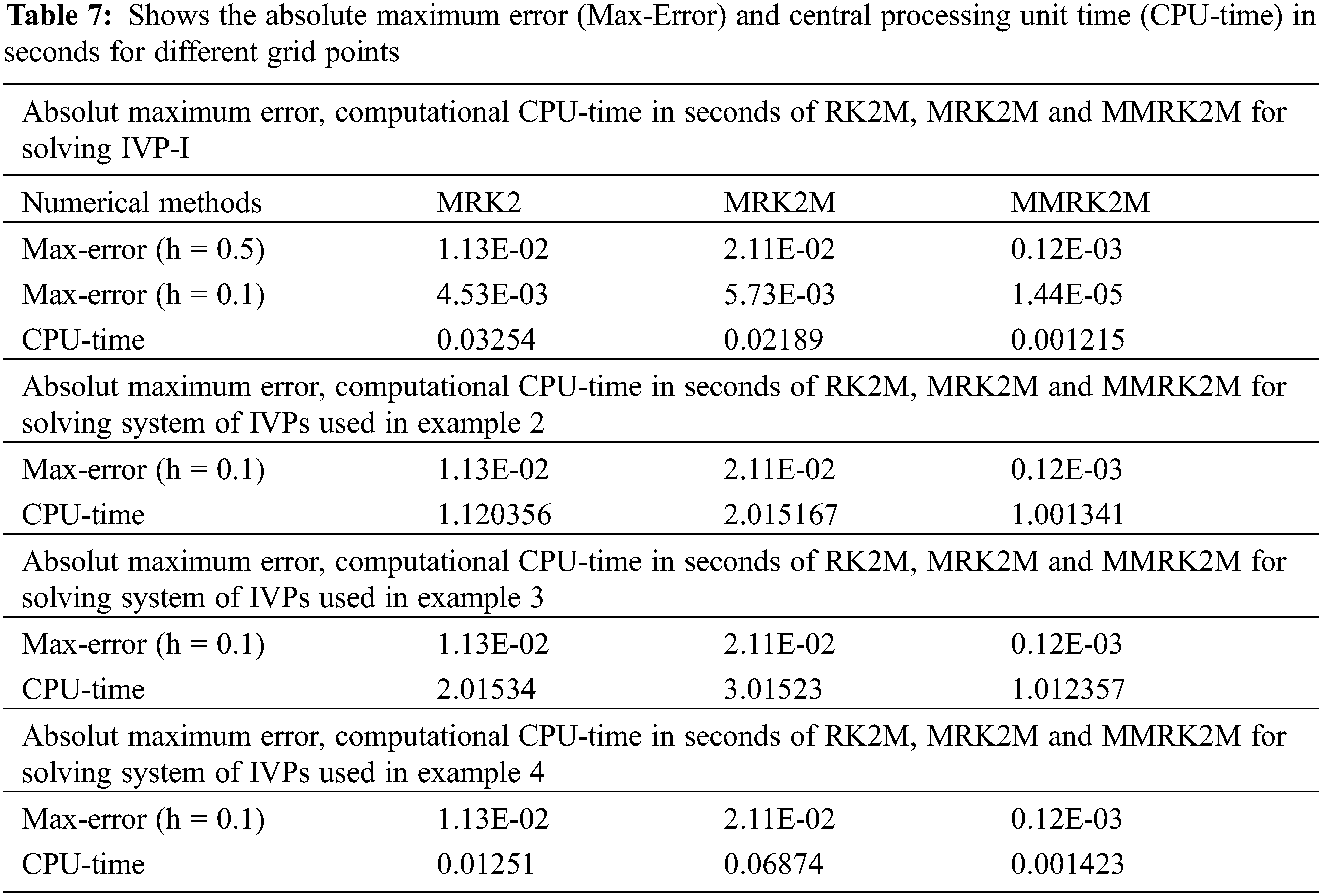
to solve IVPs and the system of IVPs [19], [20]. All numerical computations were performed using a Mat Lab 2011Rb laptop (Processor Intel® Core™ i3-3310m CPU@2.4GHz with 64-bit operating system) on Windows 8. In all Tables 1–7, the maximum absolute and local truncation errors are defined as |yn−y(xn)| .

Example 1:

Consider the IVP-I

{dy(t)dt=14(70−10cos⁡(πt12−y(t)));y(0)=60;0≤t≤12.

Using MMRK2M, MRK2 and MRK2M for different values of step-size h, we find approximate solution of the non-linear IVP-I. The numerical results are presented in Tables 1 and 2 respectively. The exact and numerical approximate solutions are shown in Figs. 3 and 4.

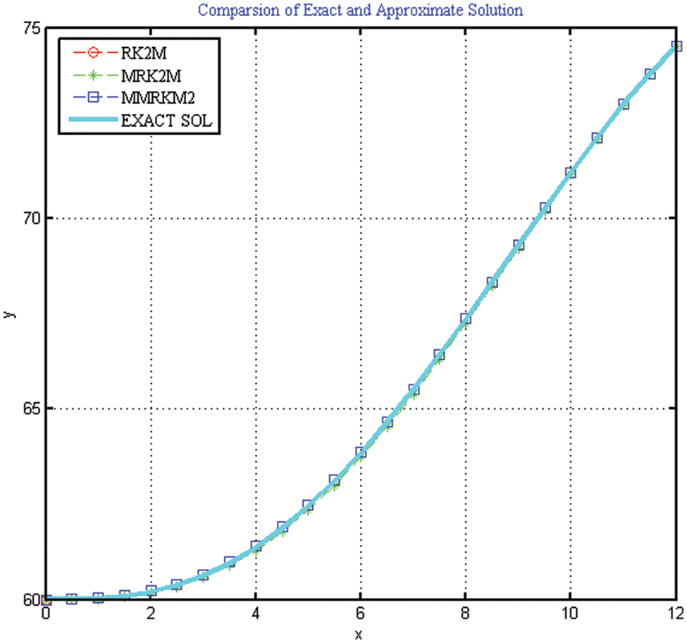
Figure 3: Comparison of exact and approximate solution of IVPs used in Example 1

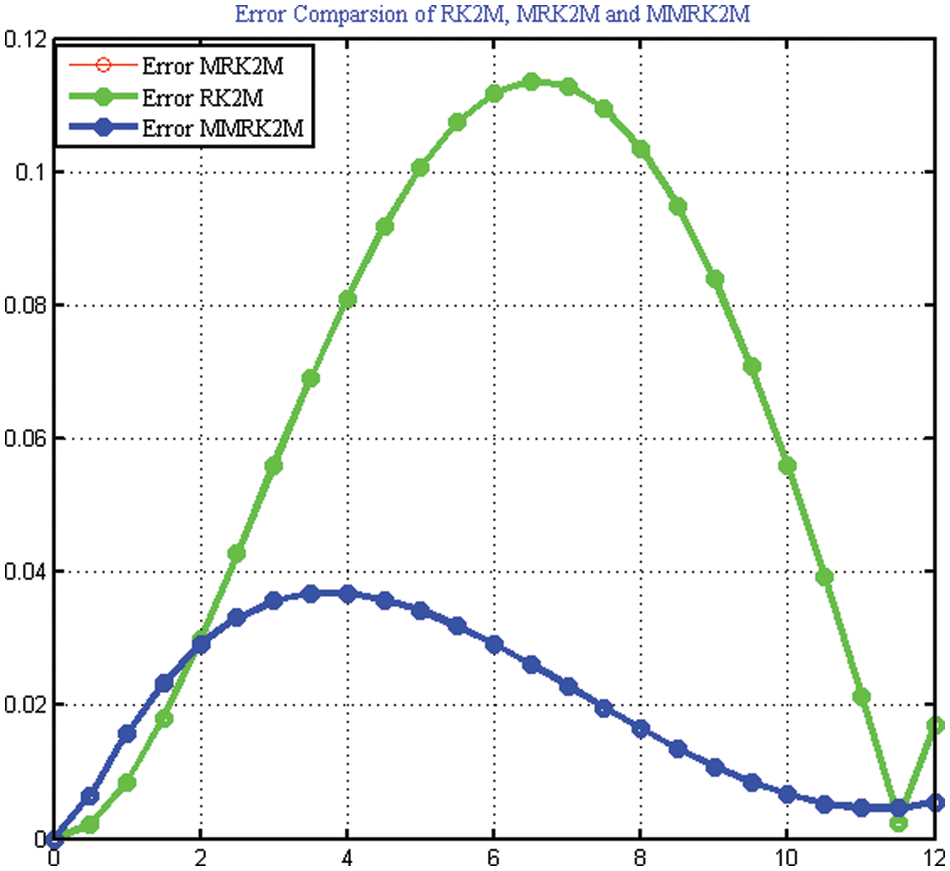
Figure 4: Error comparison of the numerical scheme MMRK2M, MRK2, MRK2M for solving IVPs used in Example 1

6.1 Applications in Engineering

Here, we discuss some engineering applications that contain highly nonlinear differential equations with information provided at the initial points.

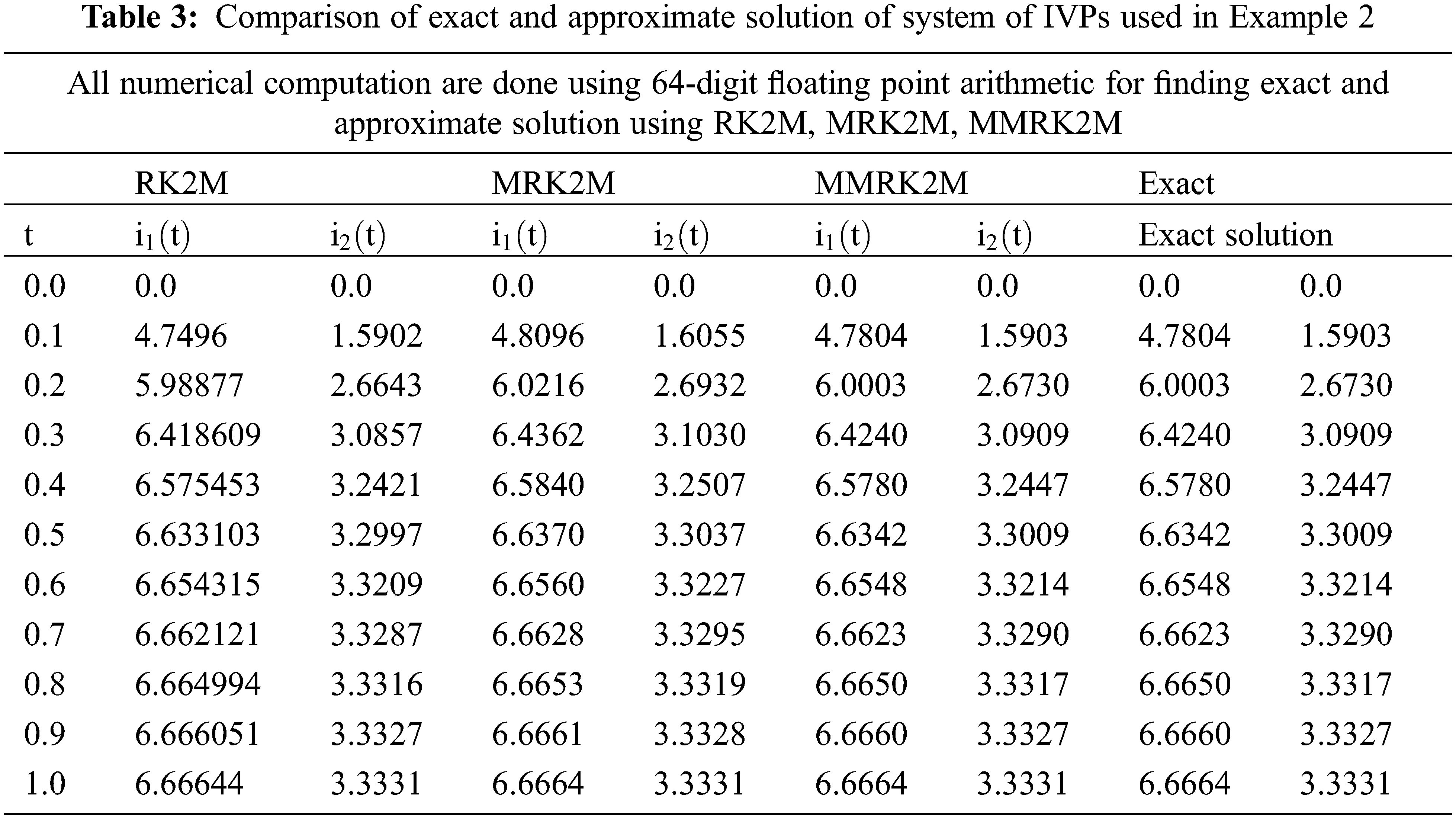
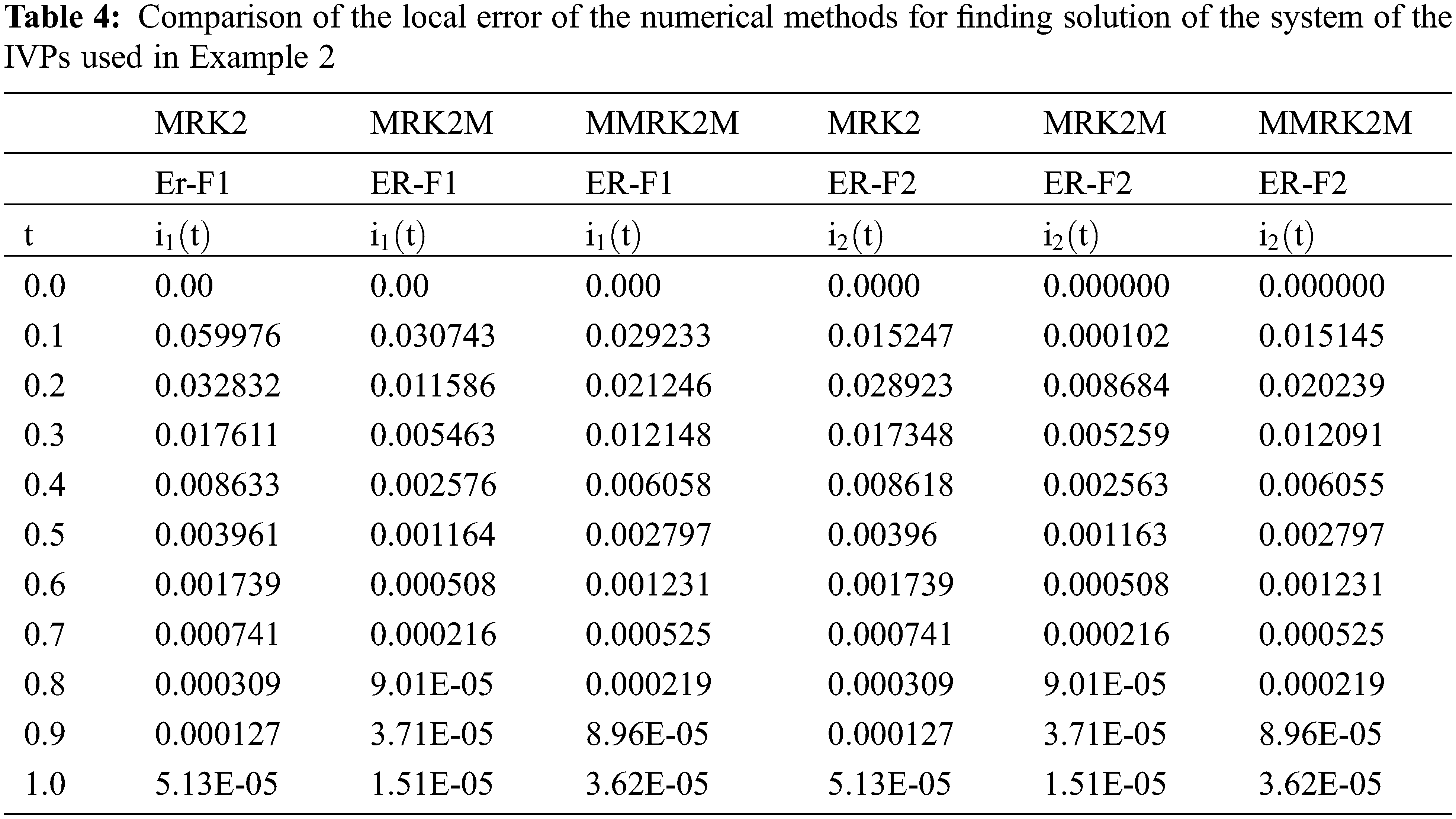
Example 2: Application in Electrical Engineering

The differential equation system for the current i1(t) and i2(t) in the electrical network depicted in Fig. 5 is

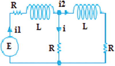
Figure 5: Shows the flow of current i1(t),i2(t) through resistance R and inductance L along with source of voltage E

{di1(t)dt=−(R1+R2)L2i1(t)+R2L2i2(t)+EL2,di2(t)dt=R2L1i1(t)−R2L1i2(t),i1(t0)=0,i2(t0)=0. (24)

The proposed and existing numerical techniques are used to solve the system of differential equations to determine the behavior of the current i1(t) and i2(t) for R1=R2=10Ω,E=100V, L1=L2=L=1h and t0=0 . By substituting the values of the resistance, voltage, and inductance, we obtain the following system of differential equations:

{di1(t)dt=−20i1(t)+10i2(t)+100,di2(t)dt=10i1(t)−20i2(t),i1(0)=0,i2(0)=0. (25)

The numerical results are presented in Tables 3 and 4 respectively. The exact and numerical approximate solutions are shown in Figs. 6 and 7.

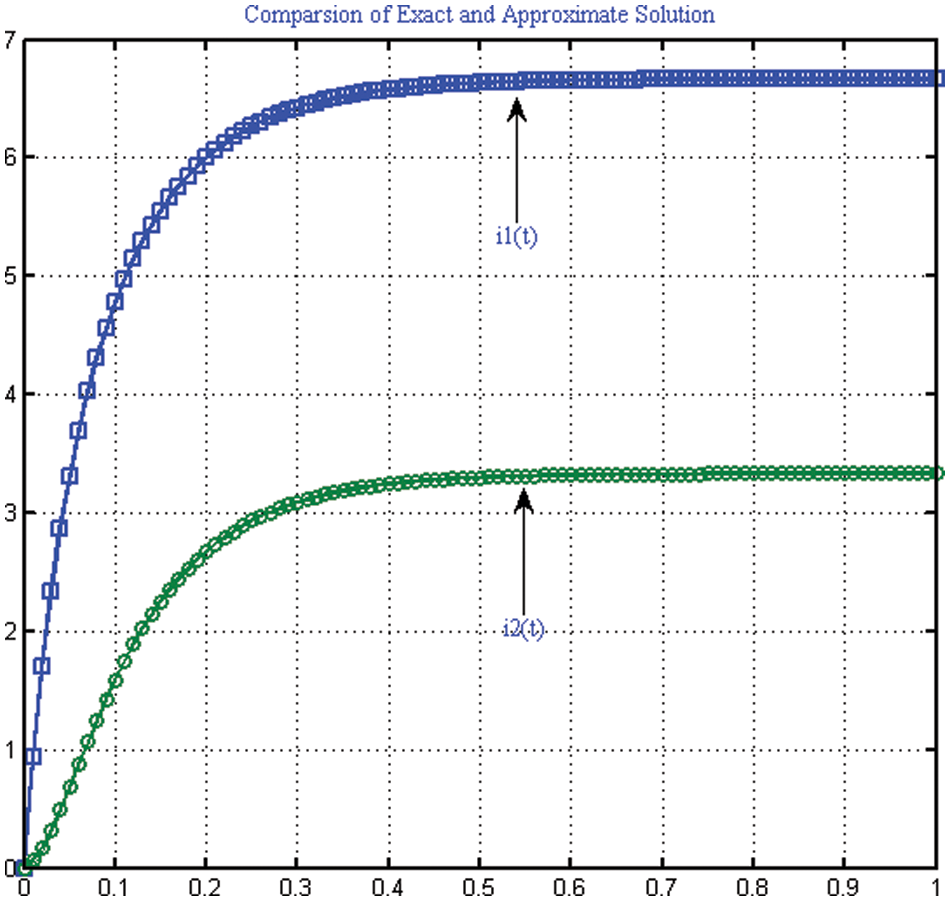
Figure 6: Comparison of exact and approximate solution of IVP used in Example 2

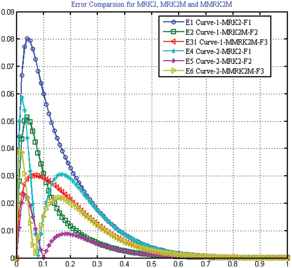
Figure 7: Error comparison of the numerical scheme MMRK2M, MRK2, MRK2M for solving IVP used in Example 2

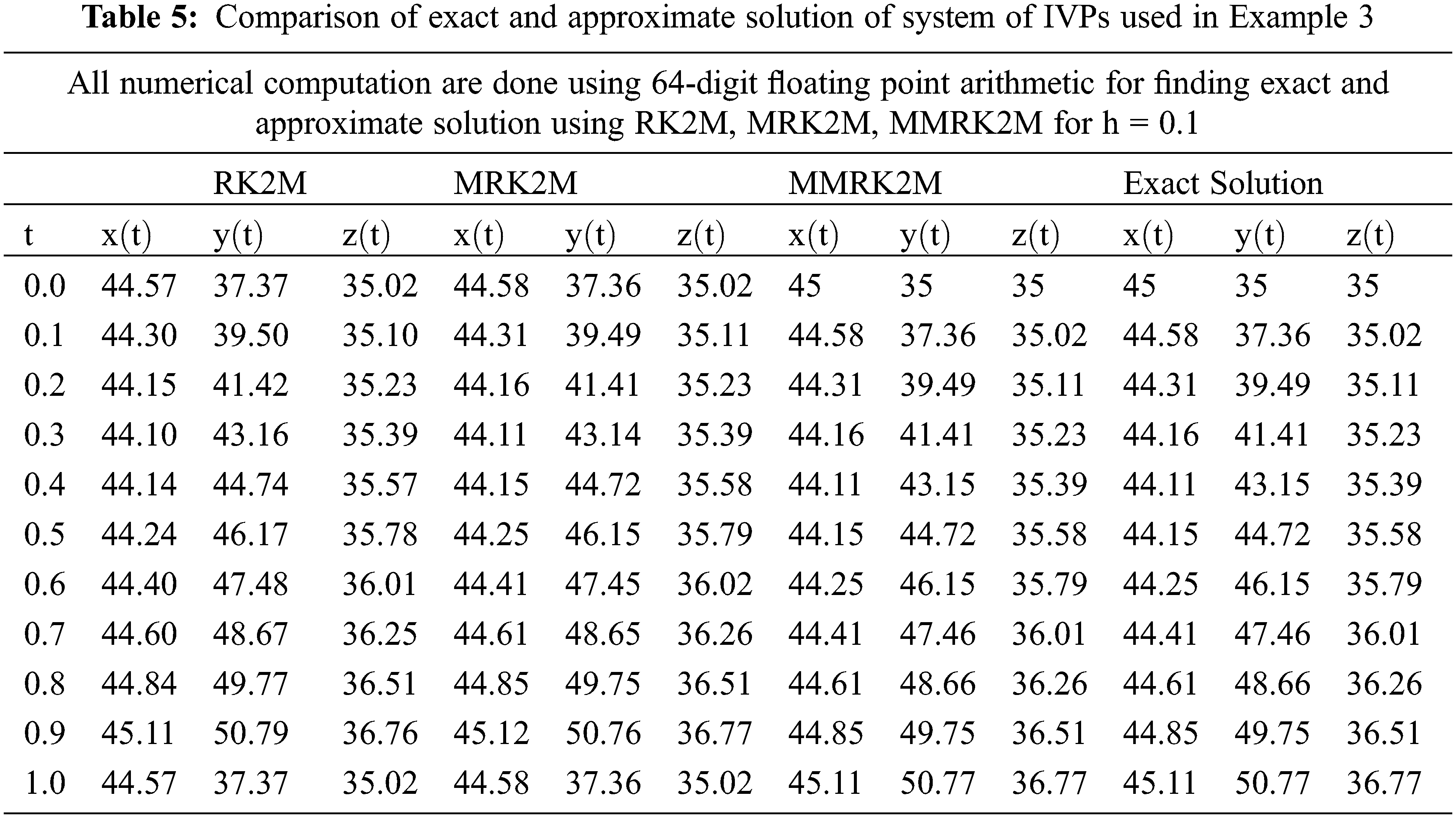
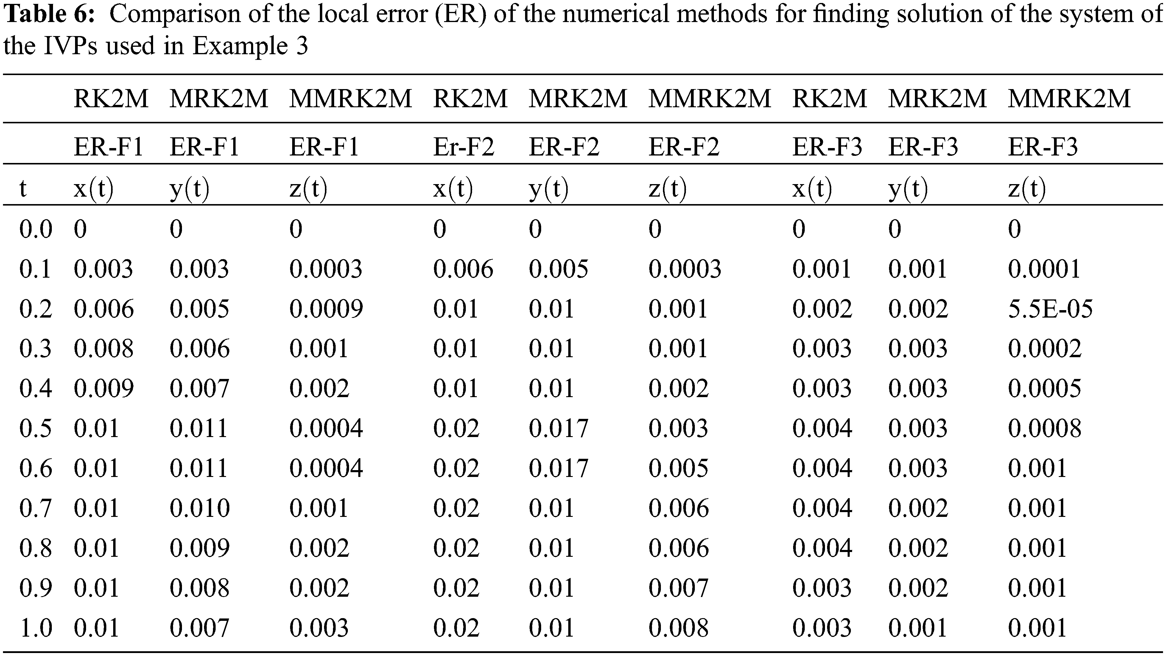
Example 3: House Heating Problem (An Engineering Application)

Consider a conventional house that has an attic, a basement, and an insulated main floor. Insulation is present in the walls and ceilings of ordinary living spaces but not in the attic portion. The floor and walls of the basement were insulated by soil. Air gaps in the joists, a layer of flooring on the main level, and a layer of drywall all serve as insulation for the basement ceiling. Using the variables and Newton’s cooling law [19], we examined how the temperatures in the three levels differ from one another. z(t) = Humidity in the attic

y(t)=Temperature in main living area

x(t)=Basement Temperature

t=Time in hours.

Primary Data: Imagine its winter and the daily high is 35°F. Furthermore, a basement earth temperature of 45°F was predicted. The heating system was then gradually turned off. The initial values at midday (t = 0) are x(t0) = 45, y(t0) = 35, and z(t0) = 35.

Portable heater: At noon, a small electric heater with a thermostat set to 100°F was turned on. When the heater is turned on, it raises the temperature by 20°F per hour, so it will take some time (may never be!) to reach 100°F.

The attic walls and ceiling, main floor walls, basement walls and floor, and basement ceiling were all subjected to temperature rate treatment. Newton’s cooling law gives rise to the positive cooling constants h0,h1,h2,h3 , and h4 , as well as the equations

{dx(t)dt=h0(45−x(t))+h1(y(t)−x(t)),dy(t)dt=h1(x(t)−y(t))+h2(35−y(t))+h3(z(t)−y(t))+20,dz(t)dt=h3(y(t)−z(t))+h4(35−z(t)),x(t0)=α0,y(t0)=α1,z(t0)=α2. (26)

The insulation constants were defined as h0=12 , h1=12 , h2=14 , h3=14 and h4=12 to indicate insulation quality. Reciprocal 1h represents the time required in hours to exchange 63 percent of the temperature differential. The main floor, for example, takes 4h. The model is:

{dx(t)dt=12(45−x(t))+12(y(t)−x(t)),dy(t)dt=12(x(t)−y(t))+14(35−y(t))+14(z(t)−y(t))+20,dz(t)dt=14(y(t)−z(t))+12(35−z(t)),x(t0)=α0,y(t0)=α1,z(t0)=α2. (27)

The homogeneous solution in vector form is provided by the formula in terms of constants a = (7 + 21)/8, b = (7 + 21)/8, c = 1 + 21, and d = 1 + 21 and arbitrary constants c1,c2,c3 .

(x(t)y(t)z(t))=c1e−t2(122)+c2e(7−218)t(4−1+212)+c3e(−1−21)t(4−1−212). (28)

The equilibrium solution is a specific solution. The exact solution to Eq. (27) is shown in Fig. 8.

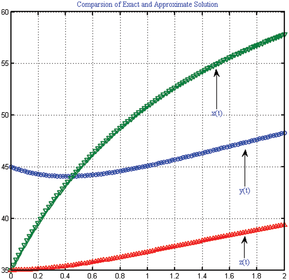
Figure 8: Comparison of exact and approximate solution of IVPs used in Example 3

(xp(t)yp(t)zp(t))=(455827541854). (29)

The temperatures of the three spaces are approximately equal to x=57,y=69 , and z=46 degrees Fahrenheit because the homogeneous solution has a limit of zero at infinity. Solving for c1,c2 , and c3 with the initial values of x(0)=α0=45,y(0)=α1=35, and z(0)=α2=35 yields specific information. c1=−8524 , c2=−2524−11521168 and c3=−2524+11521168 are solutions.

Underpowered heater: Each hour, 20°F is added to the main floor, but the heat escapes quickly, so it is approximately 51°F after one hour. The temperature was approximately 65°F after five hours. In this case, the heater is so poor that the main living space remains cold after several hours. The forced-air furnace worked similarly. The numerical results of the system of IVPs are presented in Tables 5 and 6 respectively.

Example 4: Solution of the Lorentz System

Consider three dimensional chaotic Lorentz system [20] as:

{dx(t)dt=σ1(y(t)−x(t)),dy(t)dt=σ2x(t)−y(t)−x(t);dz(t)dt=−σ3z(t)+x(t)y(t).z(t);x(0)=1;y(0)=1;z(0)=0, (30)

MMRK2M, MRK2, and MRK2M methods are used to solve the Lorentz system for different values of parameter, that is, σ1=−1.9,σ2=120,σ3=44 . The Computational CPU-time in seconds and the maximum error are listed given in Table 7. The exact solution of the Lorentz system is shown in Figs. 9–12.

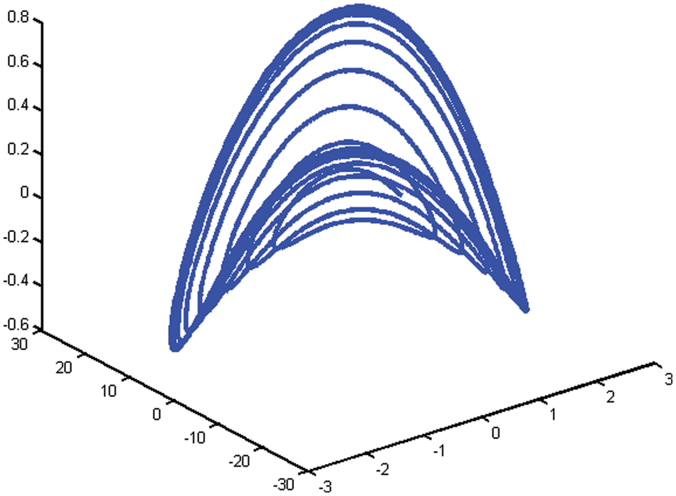
Figure 9: Solution of the Lorentz system in three dimensional space

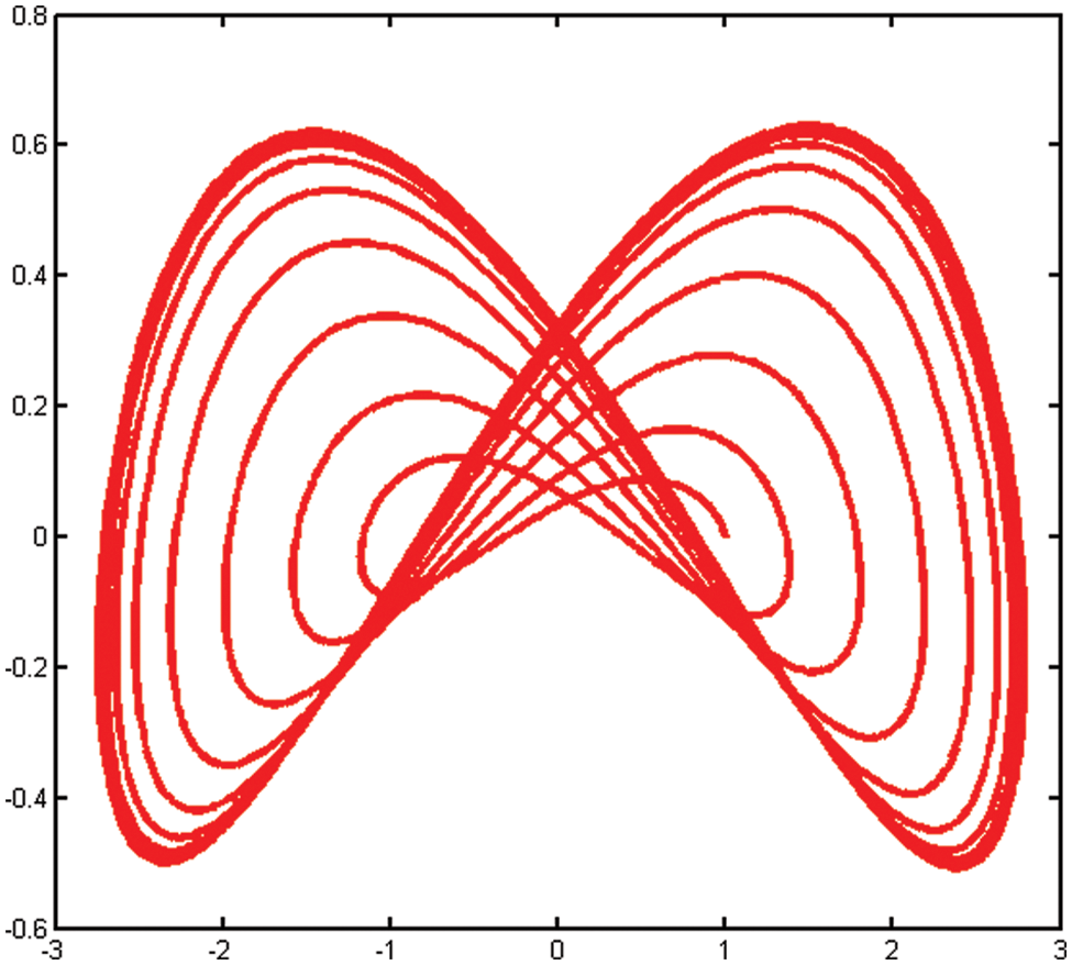
Figure 10: Phase diagram of the Lorentz system in xz-plane

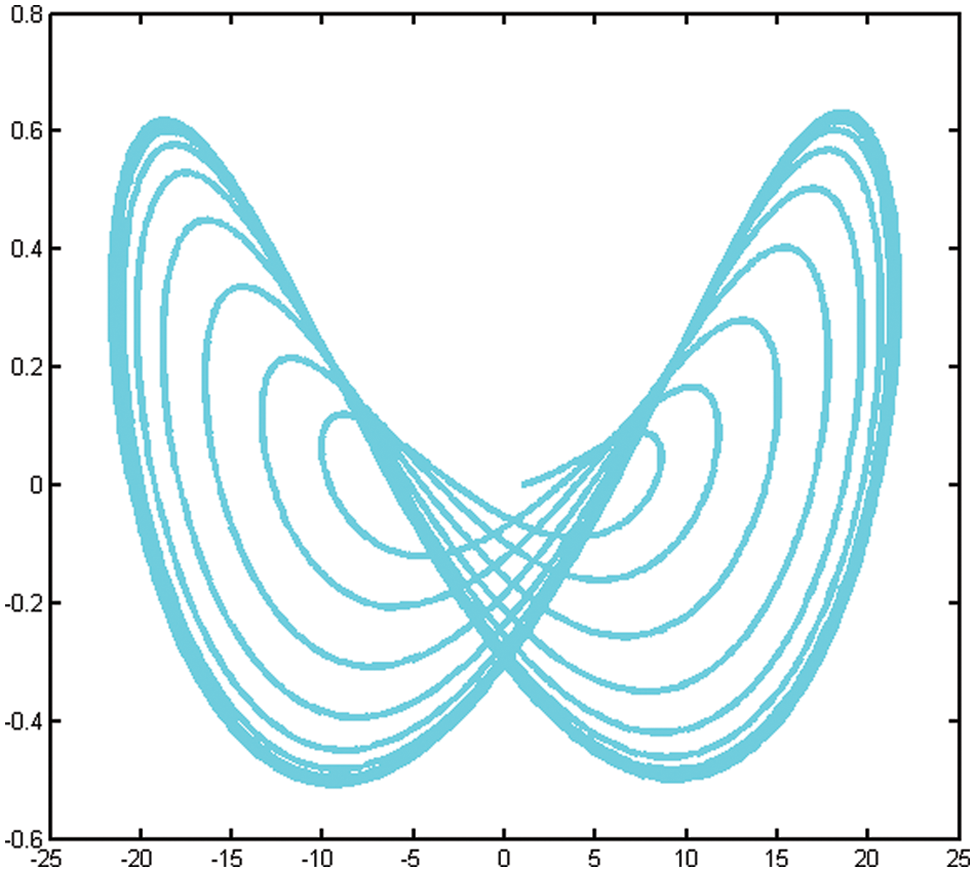
Figure 11: Phase diagram of the Lorentz system in yz-plane

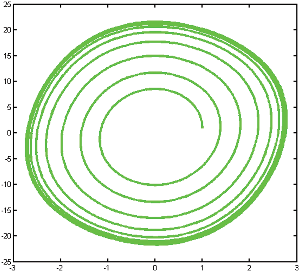
Figure 12: Projection of the Lorentz system in xy-plane

6.2 Results and Discussion

Here, we discuss the superiority of the numerical method MMRK2M over existing methods in the literature in terms of stability, residual errors and computational time. Tables 1–7, show that the newly developed method, MMRK2M, is more stable and consistent than MRK2 and MRK2M. Figs. 1 and 2 shows the larger stability zone of MMRK2M compared to MRK2 and MRK2M. Figs. 3, 6, and 7 shows the exact and approximate solutions of MMRK2M, MRK2M, and MRK2, respectively, of the IVPs used in example 1–3. Figs. 4 and 7 show the maximum residual error computed by the numerical techniques MMRK2M, MRK2M, and MRK2 for solving IVPs. In terms of residual error, MMRK2M exhibited better convergence behavior than MRK2M and MRK2.

7  Conclusion

We developed a numerical approach for solving initial value problems with linear and nonlinear functions that are efficient, stable, reliable, and consistent. The numerical system exhibited consistency, second order local convergence, and absolute stability. The Examples from engineering show that the newly developed MMRK2M theoretical order of convergence matches computational outcomes. MMRK2M computes the maximum error significantly more accurately than MRK2 and MRK2M. In terms of the computation time measured in seconds, local truncation error and absolute maximum error, Tables 1–7 and Figs. 1–12 show that our proposed technique outperforms MRK2 and MRK2M.

Acknowledgement: The authors thank to the American University of the Middle East for their support.

Funding Statement: The authors received no specific funding for this study.

Conflicts of Interest: The authors declare that they have no conflicts of interest to report regarding the present study.

References

 1.  R. L. Burden and J. D. Faires, “Boundary-value problems for ordinary differential equations,” in Numerical Analysis, 9th ed., vol. 1. Boston, MA 02210, USA: Belmont Thomson Brooks/Cole Press, pp. 1–863, 2005. [Google Scholar]

 2.  G. Adomian and R. Rach, “Inversion of nonlinear stochastic operators,” Journal of Mathematical Analysis and Applications, vol. 91, no. 1, pp. 39–46, 1983. [Google Scholar]

 3.  S. D. Kim, X. Piao, D. H. Kim and P. Kim, “Convergence on error correction methods for solving initial value problems,” Journal of Computational and Applied Mathematics, vol. 236, no. 17, pp. 4448–4461, 2012. [Google Scholar]

 4.  P. A. Naik, M. Yavuz, S. Qureshi, J. Zu and S. Townley, “Modeling and analysis of COVID-19 epidemics with treatment in fractional derivatives using real data from Pakistan,” The European Physical Journal Plus, vol. 135, no. 10, pp. 1–42, 2020. [Google Scholar]

 5.  P. A. Naik, J. Zu and K. M. Owolabi, “Modeling the mechanics of viral kinetics under immune control during primary infection of HIV-1 with treatment in fractional order,” Physica A: Statistical Mechanics and its Applications, vol. 545, no. 1, pp. 1–19, 2020. [Google Scholar]

 6.  P. A. Naik, J. Zu and M. B. Ghori, “Modeling the effects of the contaminated environments on COVID-19 transmission in India,” Results in Physics, vol. 29, no. 19, pp. 1–11, 2021. [Google Scholar]

 7.  P. A. Naik, K. M. Owolabi, J. Zu and M. U. D. Naik, “Modeling the transmission dynamics of COVID-19 pandemic in Caputo type fractional derivative,” Journal of Multiscale Modelling, vol. 12, no. 3, pp. 1–19, 2021. [Google Scholar]

 8.  W. Gautschi, “Numerical integration of ODEs, based on trigonometric polynomials,” Computer & Mathematics with Applications, vol. 8, no. 3, pp. 231–239, 1982. [Google Scholar]

 9.  A. Wambeeq, “Nonlinear methods in solving ordinary differential equations,” Journal of Computational and Applied Mathematics, vol. 2, no. 1, pp. 27–33, 1976. [Google Scholar]

10. M. A. Aslam, “Accuracy analysis of numerical solutions of initial value problems (IVP) for ordinary differential equations (ODE),” Applied Mathematics and Nonlinear Science, vol. 3, no. 1, pp. 167–174, 2018. [Google Scholar]

11. A. Ochoche, “Improving the improved modified Euler method for better performance on autonomous initial value problems,” Leonardo Journal of Science, vol. 12, pp. 57–66, 2008. [Google Scholar]

12. H. Ramos, “A non-standard explicit integration scheme for initial value problems,” Computer with Mathematics & Applications, vol. 189, no. 1, pp. 710–718, 2007. [Google Scholar]

13. M. A. Akanbi, “Third order Euler method for numerical solution of ordinary differential equations,” ARPN Journal of Engineering and Applied Sciences, vol. 5, pp. 42–49, 2010. [Google Scholar]

14. N. A. Yahya, “Semi-implicit two-step hybrid method with FSAL property for solving second order differential equations,” International Journal of Advanced and Applied Sciences, vol. 4, no. 6, pp. 169–174, 2017. [Google Scholar]

15. O. Abraham, “Improving the modified Euler method,” Leonardo Journal of Science, vol. 6, no. 10, pp. 1–8, 2007. [Google Scholar]

16. T. Ram, M. A. Solangi and A. A. Sanghah, “A hybrid numerical method with greater efficiency for solving initial value problems,” Mathematical Theory and Modeling, vol. 10, no. 2, pp. 1–7, 2020. [Google Scholar]

17. R. M. Corless, C. Y. Kaya and R. H. C. Moir, “Optimal residual and the Dahlquist test problem,” Numerical Algorithms, vol. 8, no. 4, pp. 1253–1274, 2019. [Google Scholar]

18. Z. Jackiewicz, R. Renaut and A. Feldstein, “Two-step Runge-Kutta methods,” SIAM Journal on Numerical Analysis, vol. 28, no. 4, pp. 1165–1182, 1991. [Google Scholar]

19. S. Tracogna and B. Welfert, “Two-step Runge-Kutta: Theory and practice BIT,” Numerical Mathematics, vol. 40, no. 4, pp. 775–799, 2000. [Google Scholar]

20. J. M. Li, Y. L. Wang and W. Zhang, “Numerical simulation of the Lorentz-Type chaotic system using bay centric Lagrange interpolation collocation method,” Advance in Mathematical Physics, vol. 2019, pp. 1–9, 2019. [Google Scholar]