A Multimodel Transfer-Learning-Based Car Price Prediction Model with an Automatic Fuzzy Logic Parameter Optimizer

1  Introduction

In Taiwan and everywhere else, whether in a developed or a developing country, cars have become an indispensable means of transportation. In several developed countries, such as the USA, Japan, and other European countries, the sales of used cars have surpassed those of new cars. With Taiwan joining the World Trade Organization, expansions in Taiwan’s automobile sales market have been observed. Rapid developments have also been observed in Taiwan’s used car sales market, with several platforms being established for used cars. Most people tend to buy used cars for several reasons such as a limited budget or wishing to find a vehicle for temporary reasons. As many people are unfamiliar with the detailed pricing level when buying a used car, it would be impossible for them to learn about the reasonable purchasing price. For this reason, all kinds of parameters relating to used cars are employed in this research to predict the price of the used car so that consumers will instantly know about the price of the used car to be purchased. Because the optimal algorithm is applied to the models used in this research, they will help the user obtain the data from varied scenarios without needing to manually adjust the model parameters. In the meantime, it can also achieve higher accuracy to provide car purchase information for consumers.

In this study, used car data were used to develop a used car price prediction system. Machine learning (ML) models [1–4] were used to enhance the learning ability. In addition, Fuzzy was also applied to help retrieve the features. By doing so, the fuzzification process was applied to the membership function during the research. The Membership function is to identify which element in a given set will be defined as the intended subset. Its scope ranges from 0 to 1 where “0” means the element not covered by such subset and “1” means that covered by such subset. It is executed by defining an element to several subsets and then each element in the dataset is retrieved for matching with the defined subset. As such, the resulting value is the “degree of truth” of such element in the defined subset.

This price prediction system can allow consumers to determine the price of a car before buying it and also determine whether this car is a suitable choice for them given its price.

With the rapid development of artificial intelligence (AI) technology, this technology has been extensively applied in various fields. Problems that involved a large number of data or required a large amount of time to solve through experiments can now be handled by ML in AI. Supervised learning, a type of ML, can be used to learn or build models by using a large number of training data, and new instances can be inferred depending on the results obtained. This technology has been used by numerous researchers to solve multiple problems. For example, Cao et al. [5] proposed to use of an algorithm based on a convolutional neural network (CNN) to implement smart security monitoring through the green Internet of Things and to detect whether inspection workers are wearing a helmet. Wang et al. [6] introduced a deep residual CNN model to prevent gradient explosion or disappearance and ensure the accuracy of the gradient. This model was a modification of an already existing residual CNN structure. To guarantee its ability to detect unknown attacks, transfer learning (TL) [7] was incorporated, which successfully helped solve the problem of ML of detecting only known network attacks and reduced the excessive training time of deep learning [8,9]. In another study, Pan et al. [10] established a multisource transfer double deep Q network based on actor learning. In this model, TL and deep reinforcement learning were combined to help a deep reinforcement learning agent to collect, summarize, and transfer action knowledge, including the execution of relevant tasks, such as policy simulation, feature regression, and training. Because this deep Q network had an action probability with a nonzero lower limit, corresponding to the maximum Q value, the transfer network was trained using a double deep Q network to eliminate the cumulative error resulting from the overestimation of actions. Takci et al. [11] used eight ML algorithms, including random tree and multinomial logistic regression, with four benchmark datasets to evaluate the performance of these algorithms in diagnosing autism. They further reviewed the performance of each algorithm in terms of precision, sensitivity, specificity, and classification accuracy to select the most suitable one. In another study, Lu et al. [12] proposed a new framework combining a local and a global CNN, both based on residual neural networks (ResNet)−20, to perform text recognition. A large number of patches and segmented images were first obtained depending on the aspect ratio of an image. These patches and images were then placed into a local and global CNN for training. Next, the results were fused with the AdaBoost algorithm, and the final solution was obtained. This allowed the local CNN to fully utilize the local features of the images and effectively reveal the subtle differences between languages and allowed the global CNN to classify the global features of the images to improve the identification accuracy. Shu et al. [13] developed an image-aware inference framework called IF-CNN to realize fast inferences based on computational offloading. In this framework, a model pool composed of CNN models of different complexity levels was first established. Next, the model with the most satisfactory performance among the candidate models was selected to process the corresponding image. During the selection process, a model was designed to predict the reliability of multitask learning. After the model was selected, semisubmersible optimization and feature compression were used to accelerate the distributed inference process between mobile devices and the cloud. Kollias et al. [14] introduced a new approach based on CNNs and recurrent neural networks (RNNs). In this approach, a one-minute OMG-Emotion dataset was employed, and various CNN features were used to perform emotion recognition in the wild. Pretraining was first conducted based on Aff-Wild and Aff-Wild2, large databases used for affect recognition. Next, low-, medium-, and high-level features were extracted from the trained CNN components and utilized by an RNN subnetwork in a multitask framework. The final estimate was the mean or median of the predictions. Overall, the results of this extensive experiment indicated that the arousal estimates improved when low-and high-level features were combined. In another study, Roy et al. [15] established a hybrid spectral CNN (HybridSN) for hyperspectral image classification. HybridSN is a spatial-spectral 3D CNN followed by a spatial 2D CNN. In this model, the 3D CNN is used to facilitate joint spatial-spectral feature representation from spectral bands, whereas the 2D CNN is used to learn more abstract spatial representation. Compared with the 3D CNN, the 2D CNN uses a hybrid CNN and reduces the model complexity. Yan et al. [16] proposed a CNN-based algorithm and integrated it with a hull vector support vector machine (HVSVM) to establish a usage-based insurance (UBI) rate grades. In this model, a CNN was first applied to extract the features of the UBI clients’ driving behavior data. The HVSVM was then used to classify the clients according to their driving behavior and obtain their insurance rate grades. Overall, the results indicated that the discrimination accuracy of the CNN-HVSVM algorithm was higher than that of the CNN, back-propagation neural network, and support vector machine (SVM) algorithms in rating the UBI clients’ risk-driving behavior. The CNN-HVSVM algorithm was also faster than the CNN-SVM algorithm in cases of large training sets. Moreover, the model was easy to implement and had satisfactory robustness, and it was able to adapt to various datasets and yield more satisfactory results during insurance rate determination. These results indicated that the CNN-HVSVM model is highly applicable and flexible, can accurately and effectively predict the ratings of UBI clients, and can yield prediction results that are consistent with the actual situation.

In Chapter 2, we will introduce the source and the distribution status of the dataset used in this research. In Chapter 3, the theory of the model used in this research, the data pre-processing and the “k-fold cross-validation” are described. In Chapter 4, we will demonstrate the training result diagram of each model and will introduce the model efficacy evaluation method, and then list the result in the table for easier comparison. The conclusions are provided in Chapter 5. Among all models being used in this research, the method proposed by us can deliver the most accurate prediction result. In this way, it allows the consumers wishing to buy the used car to learn about the price of the target car beforehand. Finally, in Appendix, a supplementary description is also provided to explain the basic model structure and its theory that are used in this research.

2  System Architecture

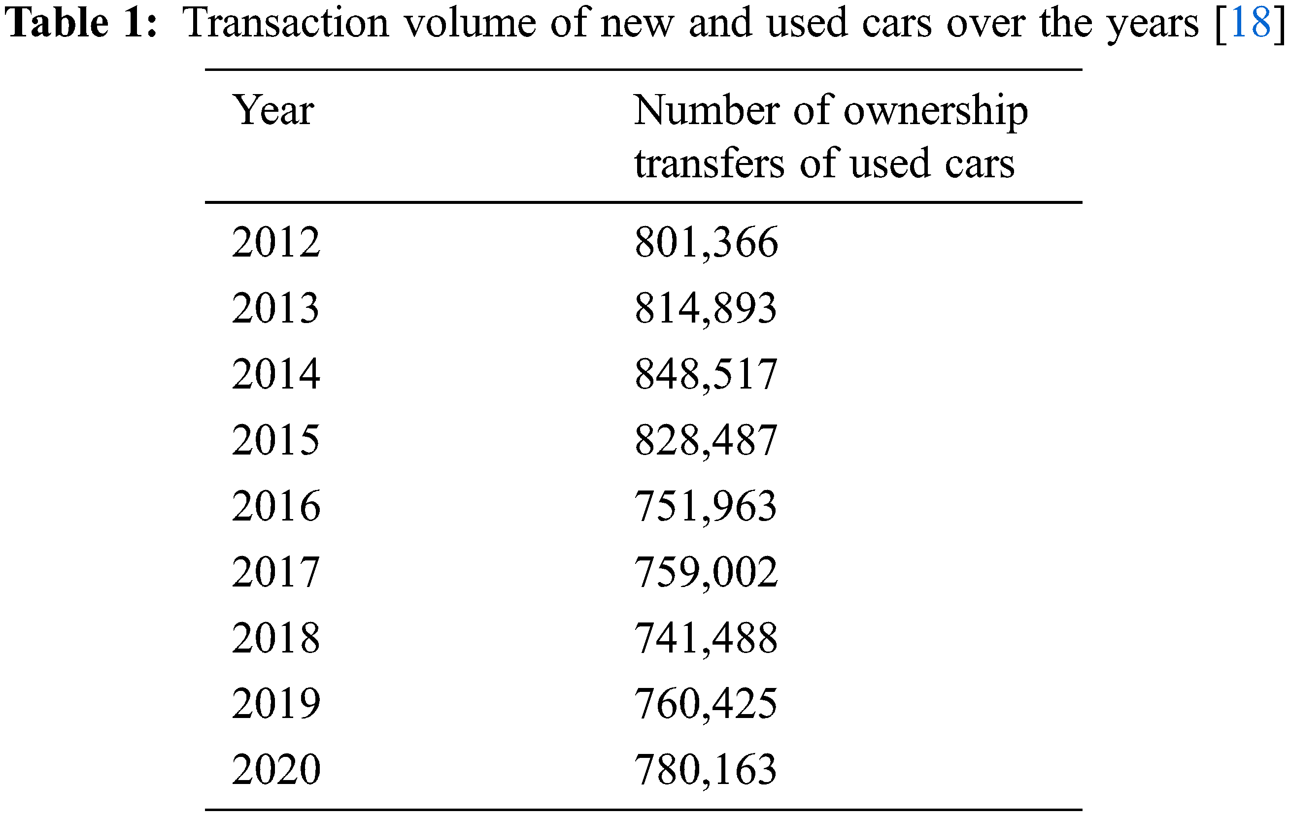
As shown in Table 1, the sales of used cars in Taiwan exceed those of new cars every year. According to used car dealers, the economic downturn has encouraged the sales of used cars. What is more attractive to these dealers is that used cars outsell new cars. For consumers, although buying a used car may be risky, cars remain an irreplaceable means of transportation, which leaves them with no choice but to buy a used car.

The data used in this study were retrieved from [17]. This dataset was collected with a web scraper through exchange and mart, including the model of a used BMW car, registration year, transmission style, mileage, fuel type, and road tax. All of these parameters are described in Table 2. In Fig. 1, we learned that the factors closely connected with the price of the used car are mileage and year. The more the mileage, the lower the price; and the newer the year, the higher and price. By inputting the car-related information in the model used in this research, the consumers will be able to predict the price of such a used car. The correlation between them is presented in Figs. 2–4.

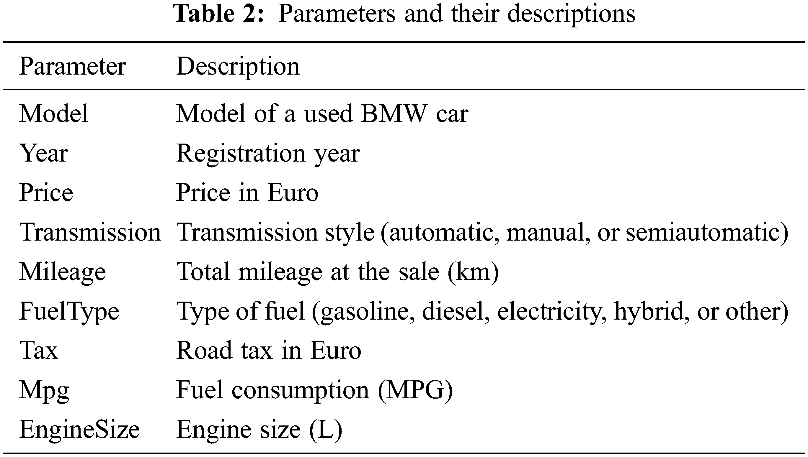
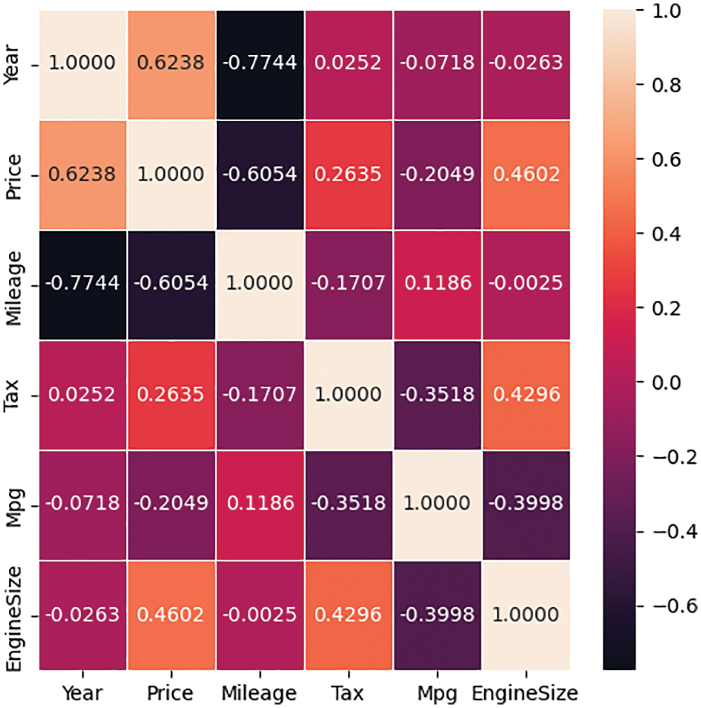
Figure 1: Heat map of the parameters included in the study

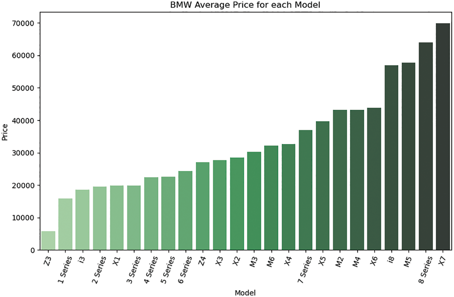
Figure 2: Correlation between the average selling prices of used cars and their model

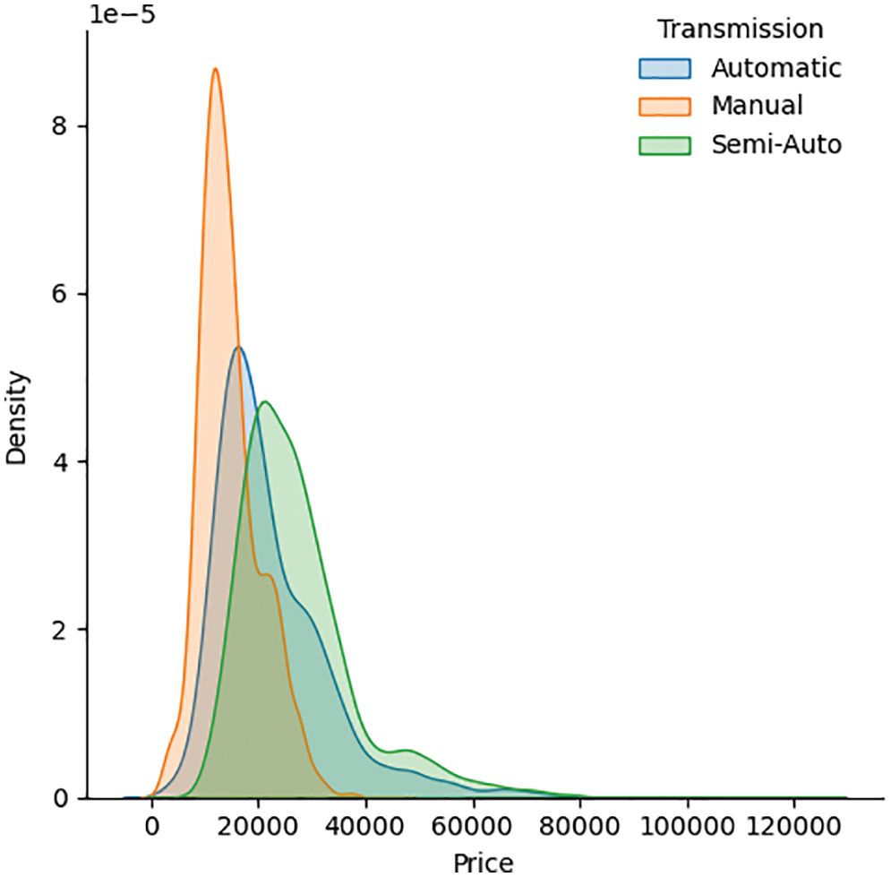
Figure 3: Correlation between the selling prices of used cars and their transmission type

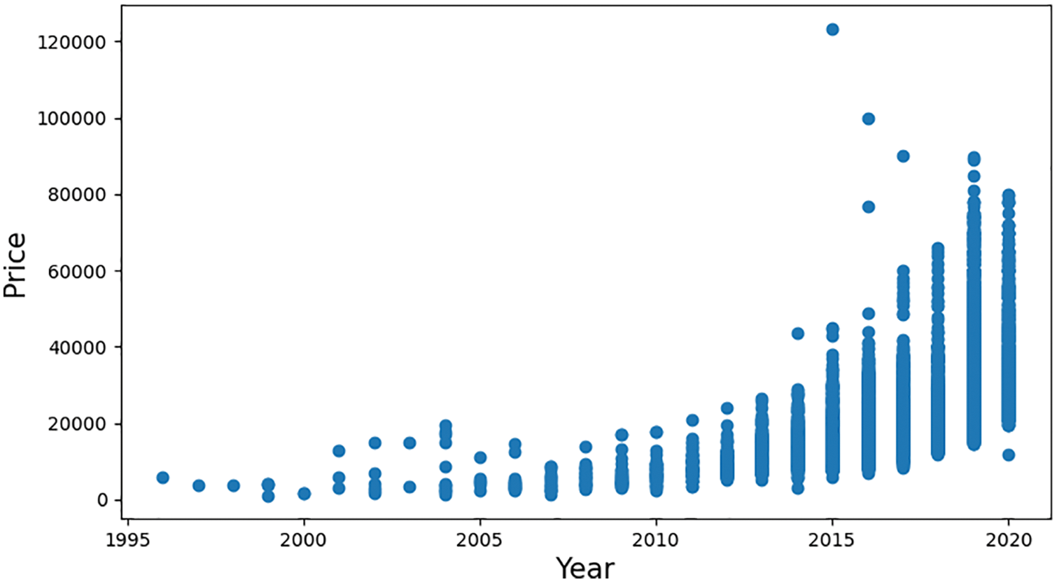
Figure 4: Correlation between the selling prices of used cars and their registration year

Because multiple parameters were character strings rather than numerical values, the models faced some difficulties in identifying them. Therefore, to solve this problem, data normalization was required. Among the common data normalization methods are label encoding and one-hot encoding. Label encoding is the process of mapping each category in the data to each integer, and it does not add any extra columns. In this study, a neural network combining TL, random forest (RF) [19], K-nearest neighbors (KNN) [20], and multilayer perceptron (MLP) [21] algorithms were proposed, and the parameters in the model were adjusted to complete and optimize its structure. The model was also compared to various conventional ML methods.

3  The Proposed Method

In this study, the algorithm of the ML model was developed basis on a neural network. Neural networks are connected by a large number of artificial neurons and are considered a mathematical or computational model that imitates how biological neurons transmit messages to each other. Such a model is used to evaluate or approximate functions to facilitate identification, decision-making, and prediction. It also has several advantages; for example, it has great tolerance to different data types, has superior adaptability, and can fully approximate any nonlinear functions.

Any ML algorithm has two prediction goals: regression and classification. Regression is mainly used to predict continuous data, such as stock and house price prediction. To predict a continuous function, mathematical functions are employed to combine different parameters. The goal of regression is to minimize the error between the prediction result and the actual value. Classification is typically used to predict data with noncontinuous values, such as in handwriting recognition and stamen classification. Several parameters are applied to create a decision boundary for differentiation. The goal of classification is to minimize the error of misclassification. In this study, the prediction was considered a regression problem.

3.1 Data Preprocessing

To facilitate subsequent model building, raw data should first be preprocessed. This can accelerate model convergence, increase prediction accuracy, and avoid result distortion. Therefore, a min-max normalization preprocessing method was used [22]. The minimum and maximum values of the raw data were extracted and transformed into 0 and 1 to scale, respectively. This process not only reduced the scope of the data but also preserved their trend without losing any characteristics. For this purpose, the following equation was used:

A′=A−AminAmax−Amin∈[0, 1] (1)

where A′ is the normalized value and A­min, Amax, and A are the minimum, maximum, and original values, respectively.

Following data preprocessing, cross-validation is performed. Next, after ML is performed, the dataset is typically divided into a training set and a validation set. The training set is used to train the ML model, whereas the validation set is used to verify whether the model has been trained well. When the sample size is small, the data extracted as the validation set are generally unrepresentative. This means that the verification results of some of the extracted data may be satisfactory and those of other data may be unsatisfactory. To avoid this problem and more effectively evaluate the quality of the model, cross-validation is adopted. Among the various cross-validation methods available, a 10-fold cross-validation method was selected in this study.

Generally, the term “K-fold” means dividing data into K equal parts, namely, dividing the training set into K parts. The same model is trained K times, and during each training procedure, K−1 training sets are selected from the K parts to serve as the new training set. The remaining set serves as the validation set. Different rounds of training results are then combined into a verification list and averaged to obtain the final result. This process is demonstrated in Fig. 5. As shown in the figure, the variance was reduced by averaging different rounds of training results. Therefore, the model became less sensitive to the division of data.

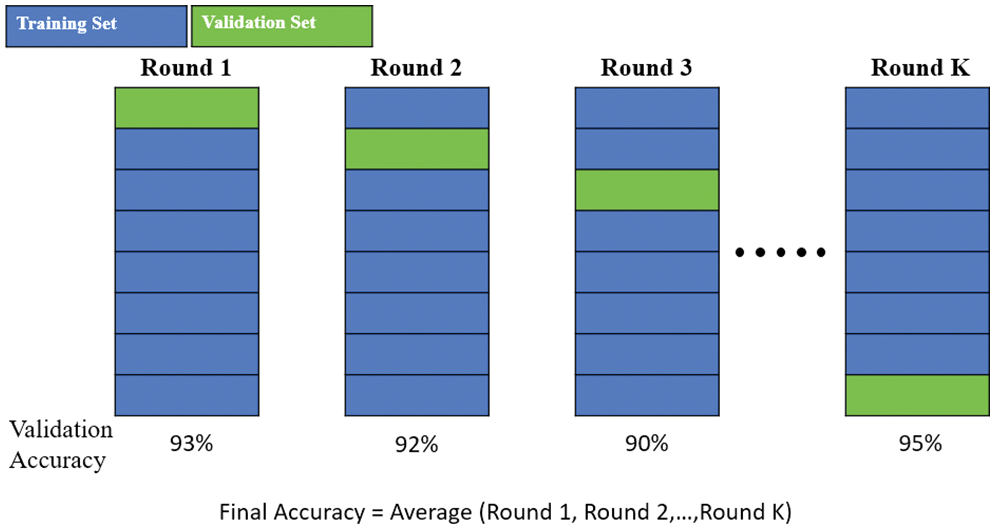
Figure 5: K-fold process

In this study, a composite model combining decision tree (DT) [23], RF, support vector regression (SVR) [24], KNN, MLP, and TL algorithms were employed, and these six algorithms were compared.

3.2 Composite Model Combining Machine Learning Algorithms

Before training, the data were fuzzified by the membership function (MF) of a fuzzy set. The MF is used to transform the input provided into a fuzzy inference system. Several methods can be used to run an MF. The most widely accepted and applied method is the triangular membership function (TMF). The TMF defines the input as a triangle and transforms this input into three levels (i.e., low, medium, and high) with a converted value. A linear representation of TMF is presented in Fig. 6. Points a, b, and c in Fig. 6 are where the maximum values of the low, medium and high levels lie, respectively.

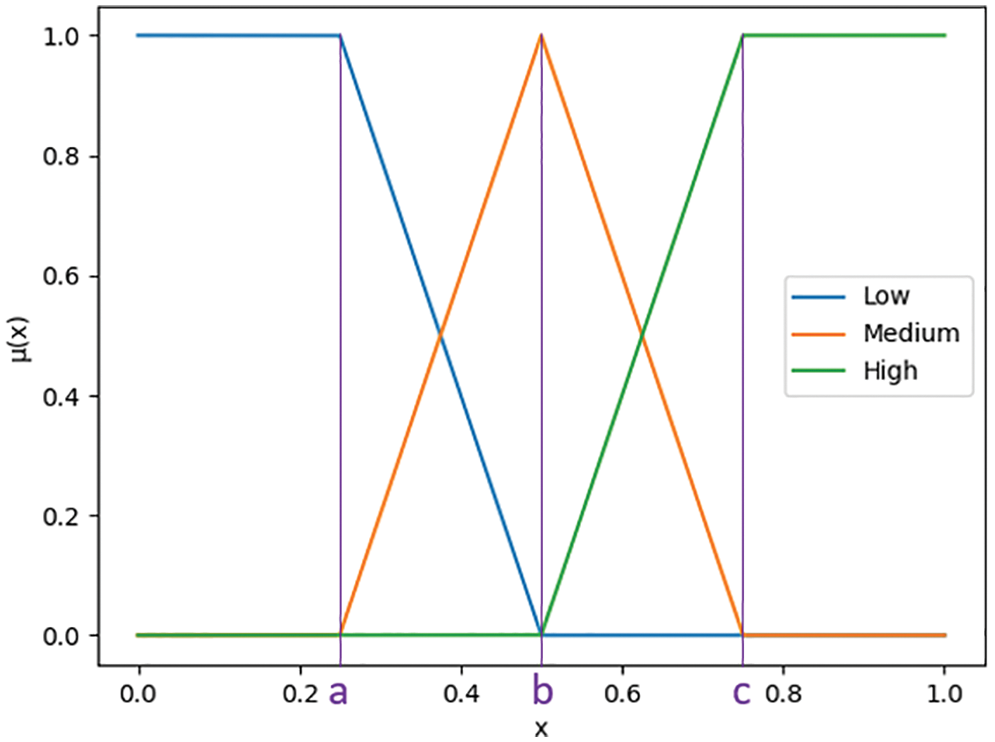
Figure 6: Linear representation of TMF

In this study, these points were optimized using an optimization algorithm, which allowed the users to easily perform predictions with this model without having to thoroughly understand the TMF. Three optimization algorithms were compared: gray wolf optimization (GWO) [25], center particle swarm optimization (CPSO) [26], and cat swarm optimization (CSO) [27].

GWO is an optimization algorithm deduced from the social class and hunting behavior of gray wolves (see Fig. 7). According to the gray wolf hierarchy diagram shown in Fig. 8, the optimal solution, second optimal solution, third optimal solution, and remaining candidate solutions are regarded as α, β, δ, and ω, respectively. In GWO, optimization is led by α, β, and δ, with ω following the three wolves.

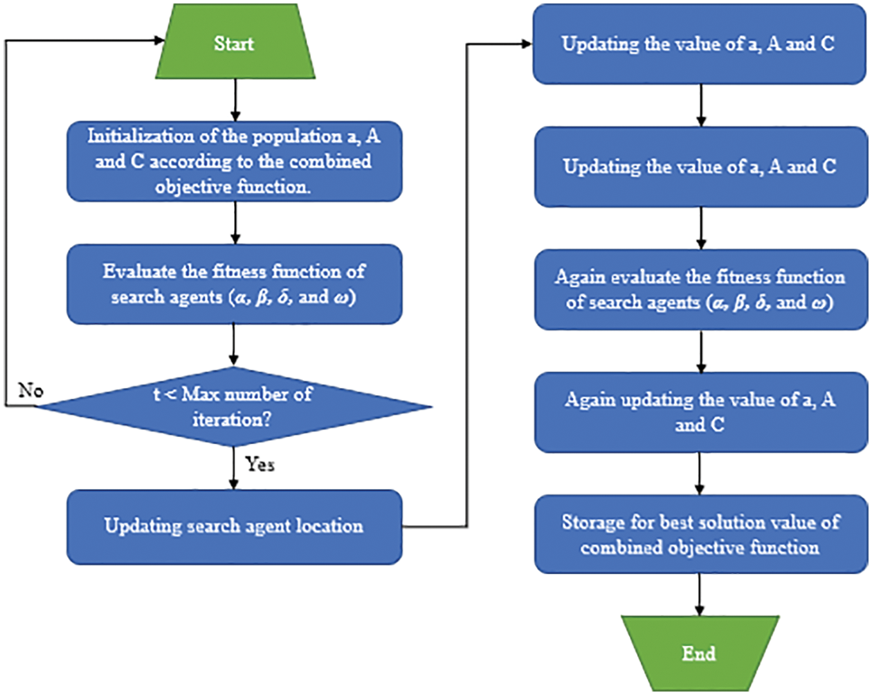
Figure 7: Procedure of GWO

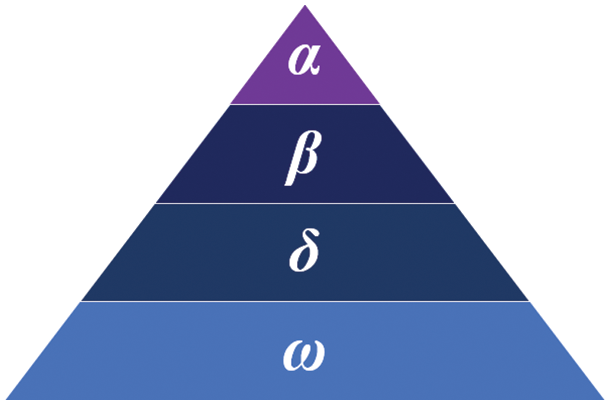
Figure 8: Gray wolf hierarchy diagram, where α is the leader, β is the deputy leader, and ω is the lowest class, which typically plays the role of a scapegoat

The hunting behavior can be divided into the following three steps: (1) stalking, chasing, and approaching the prey; (2) chasing and surrounding the prey until it stops moving; and (3) attacking the prey.

Surrounding the prey: Gray wolves surround their prey during hunting. To mathematically model this surrounding behavior, the following equations were proposed:

D→=|C→⋅x→P(t)−x→(t)| (2)

x→(t+1)=x→P(t)−A→⋅D→ (3)

where t is the current number of iterations, A→ and C→ are coefficient vectors, x→P is the location of the prey, and x→ is the location of the gray wolves.

Both A→ and C→ were calculated using the following equations:

A→=2a→⋅r→1−a→ (4)

C→=2⋅r2→ (5)

where the component of a→ decreases linearly from 2 to 0 during the iterations and r→1 and r2→ are random vectors in [0, 1].

Hunting: Gray wolves first identify their prey and surround it. Hunting is generally led by α, with β and δ occasionally participating in the process. However, in an abstract search space, the location of the prey is unknown. To mathematically simulate the hunting behavior of gray wolves and further understand the potential locations of α, β, and δ, the first three optimal solutions obtained are preserved, and the other search agents (including ω) are forced to update their locations depending on the location of the optimal search agent. The Schematic for the Location update of GWO is presented in Fig. 9. For this purpose, the following equations are used:

Dα→=|C→1⋅xα→−x→| (6)

D→β=|C2→⋅x→β−x→| (7)

D→δ=|C3→⋅xδ→−x→| (8)

x1→=xα→−A→1⋅D→α (9)

x→2=x→β−A2→⋅Dβ→ (10)

x3→=xδ→−A→3⋅Dδ→ (11)

x→(t+1)=x→1+x→2+x3→3 (12)

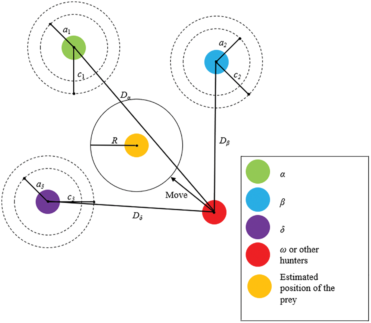
Figure 9: Schematic for Location update of GWO [25]

Attacking the prey: Gray wolves complete their hunting by attacking their prey after it stops moving. As a mathematical model of their approach to their prey, the value of a→ first decreases. The fluctuation range of A→ also decreases a→ . In other words, A→ becomes a random value in [2 a→ , 2 a→ ], where a→ decreases from 2 to 0 during the iterations. When A→ becomes within [1, 1], the expansion of the search agent can be anywhere between its current location and the prey’s location.

Searching for the prey: Gray wolves typically search depending on the locations of α, β, and δ. They diverge to search for their prey and gather to attack it. To mathematically model this divergence, A→ , a random value greater than 1 or smaller than −1, is used to represent the divergence of the search agent from the prey. This emphasizes the search process and allows GWO to perform a global search.

In CPSO, which is based on swarm search behavior, the center of the swarm is regarded as an extra particle. If the original population size contains N particles, then CPSO adds a central particle to the swarm. Although this central particle has no velocity, its location is simultaneously updated, and it participates in the competition for global best. After standard particle swarm optimization (PSO) [28] completes an iteration and updates the locations of N particles, the central particle is considered as the (N + 1)th particle. For this purpose, the following equation is used:

xc=xN+1=∑i=1N⁡xiN (13)

where x­c is the location of the central particle calculated by the original swarm. Compared with standard PSO, the population size of CPSO becomes N + 1. In this scenario, the central particle is introduced into the swarm because the center of the swarm is a critical location, which represents the location at which the entire swarm shrinks during the iterations.

CSO is an optimization algorithm deduced by imitating the natural behavior of cats. Generally, the behavior of cats of staying still and moving slowly corresponds to a seeking mode, whereas their behavior of quickly chasing their prey corresponds to a tracing mode. Those seeking and tracing modes are included in each iteration. The number of agents is fixed at a predefined ratio called MR. In this scenario, the cats move in a solution space, and their locations represent the solution set. Each cat has a fitness value and a location and velocity in each dimension. Each cat also has a flag that identifies whether this cat is in the seeking or tracing mode. The process of CSO is presented in Fig. 10.

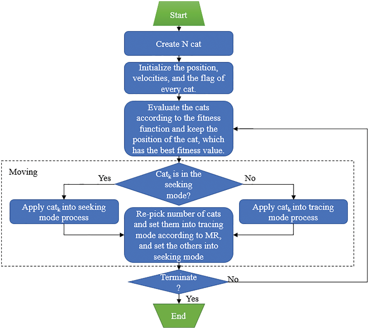
Figure 10: Process of CSO [29]

MLP is a forward-propagation neural network that consists of at least three layers: an input layer, a hidden layer, and an output layer. Back-propagation technology is applied to achieve ML in supervised learning. The structure of MLP is presented in Fig. 11.

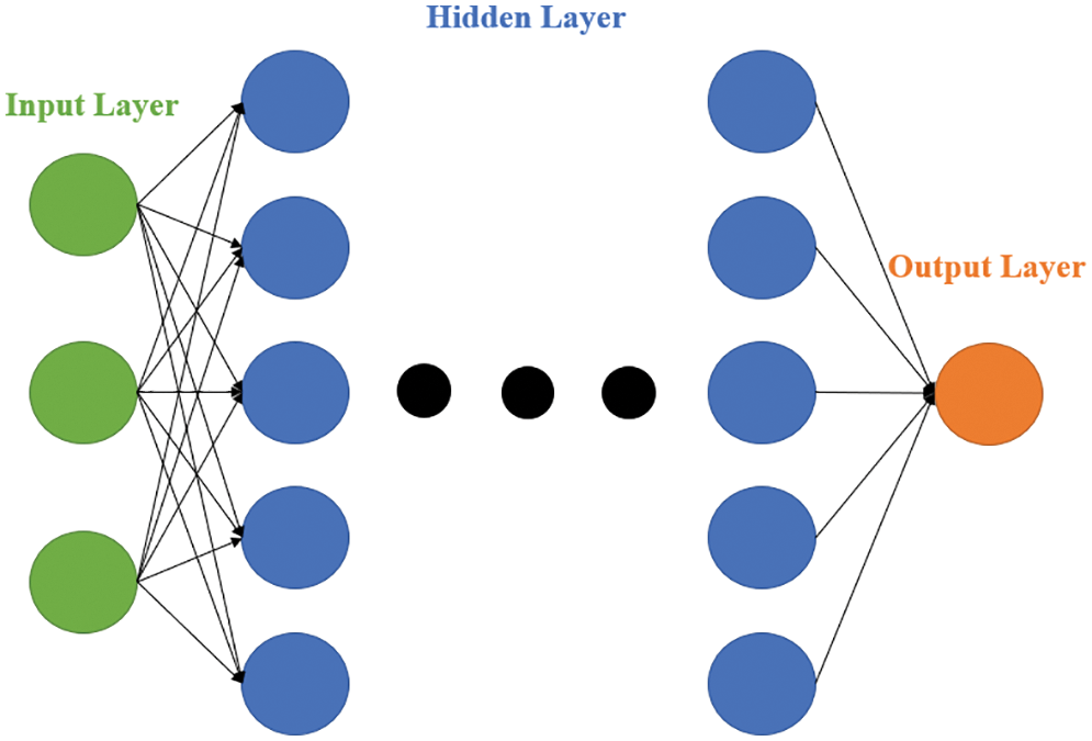
Figure 11: Structure of MLP

In TL, the trained model is transferred to another new model to avoid retraining the new model from scratch. TL is mainly used to solve difficult data labeling and acquisition problems. Several methods can be used to construct a TL model. In this study, multi-task learning was used as the model framework. In general, multitask learning increases the generalization error by using the information in the training signals of relevant tasks as inductive bias. The framework of the model proposed in this study is presented in Fig. 12.

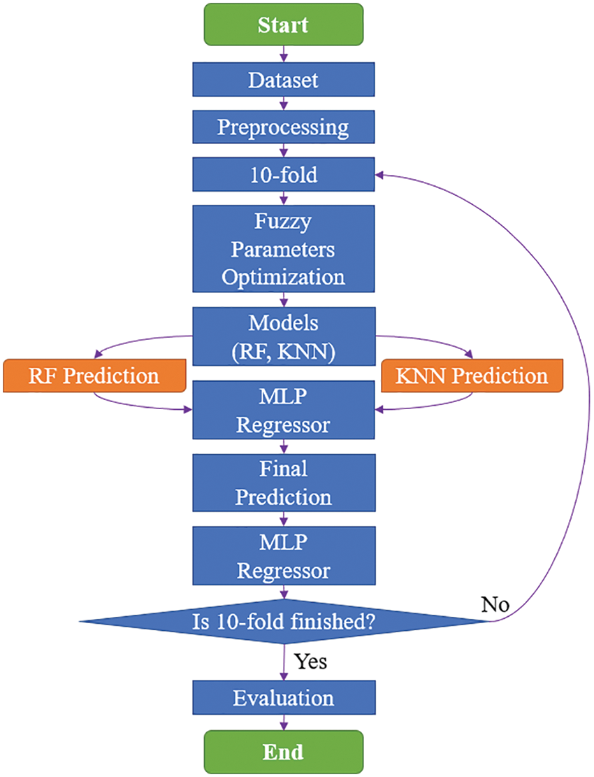
Figure 12: Process of TL

4  The Experimental Results

In this study, various optimization algorithms were compared. As shown in Fig. 13, GWO was selected as the most suitable optimization algorithm and used as the optimization algorithm for TL. The results of GWO and those of the remaining algorithms were then compared to select the most suitable ML model for this study.

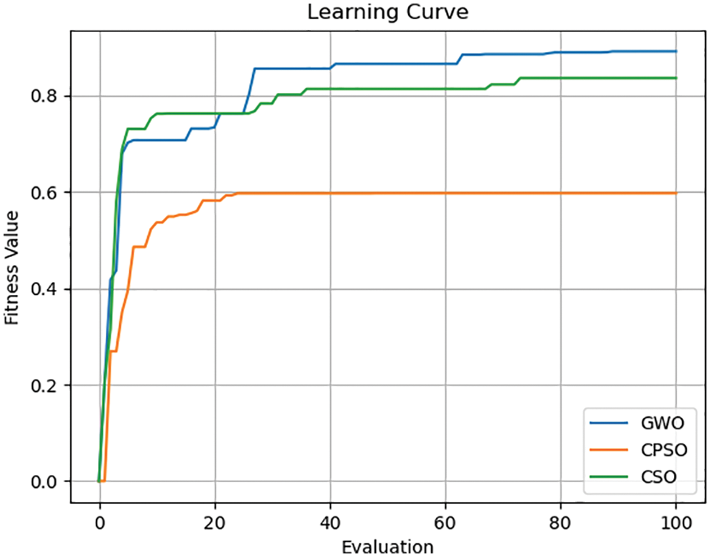
Figure 13: Comparison between the learning curves of GWO, CPSO, and CSO

To estimate the accuracy of the data predicted by the algorithms, several statistical measures, such as the mean square error (MSE), root-mean-square error (RMSE), mean absolute error (MAE), and coefficient of determination (R2), were used. In addition, the performances of the algorithms were compared.

MSE, also referred to as L2 loss in mathematics, is the most commonly used regression evaluation indicator. It is obtained by calculating the sum of the squares of the distance between the predicted value and the true value. Because of this squaring, MSE penalizes deviations from the true value, making it suitable for gradient calculation. A smaller MSE value indicates that the prediction model describes the experimental data with greater accuracy. MSE is calculated as follows:

MSE=∑i=1N⁡(yi−y^i)2N (14)

RMSE is the square root of the square of the deviation of the predicted value from the true value and the ratio of the total data (i.e., the square root of MSE). Because of this square rooting, RMSE is suitable for evaluating data with high values, such as house prices. A larger RMSE value implies a less accurate prediction, whereas a smaller RMSE value implies a more accurate prediction. RMSE is calculated as follows:

RMSE=MSE=1N∑i=1N⁡(yi−y^i)2 (15)

MAE, also referred to as L1 loss in mathematics, is a loss function of regression. MAE is the mean of the absolute values of the errors in each measure and is used to estimate the accuracy of an algorithm. A smaller MAE value suggests that the predicted value is more accurate. MAE is calculated as follows:

MAE=∑i=1N⁡|yi−y^i|N (16)

R2 is a statistical measure commonly used as an indicator to measure the performance of a regression model. The value of R2 typically lies within the range [0, 1]. This value indicates the degree of fitness of the true and predicted values. A value closer to 1 implies greater accuracy. The following equation is used to calculate R2:

R2 ≡1−∑i=1n⁡(yi−yi^)2∑i=1n⁡(yi−y¯)2 (17)

In this section, the algorithms introduced in Section 3 were individually trained. As shown in Figs. 14–18, for errors exceeding 0.005 between the predicted and true values, the data points are shown in orange; for errors ranging between 0.005 and 0.025, the data points are shown in green; and for errors smaller than 0.025, the data points are shown in blue. These results indicate that the performances of the models can be initially determined depending on the color of the data points. However, the values of MSE, RMSE, MAE, and R2 offer more precise model accuracy results (Table 3).

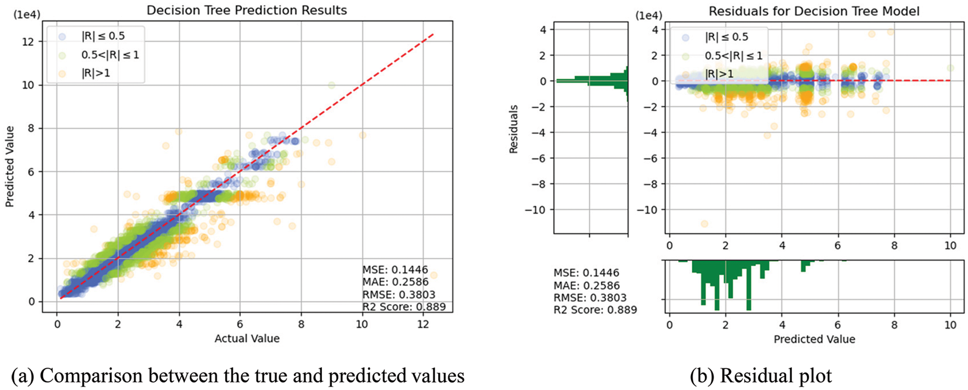
Figure 14: Prediction results of DTs

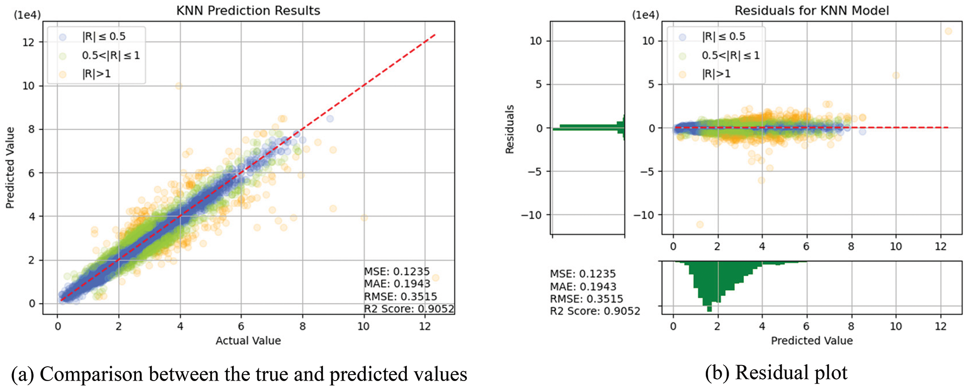
Figure 15: Prediction results of KNN

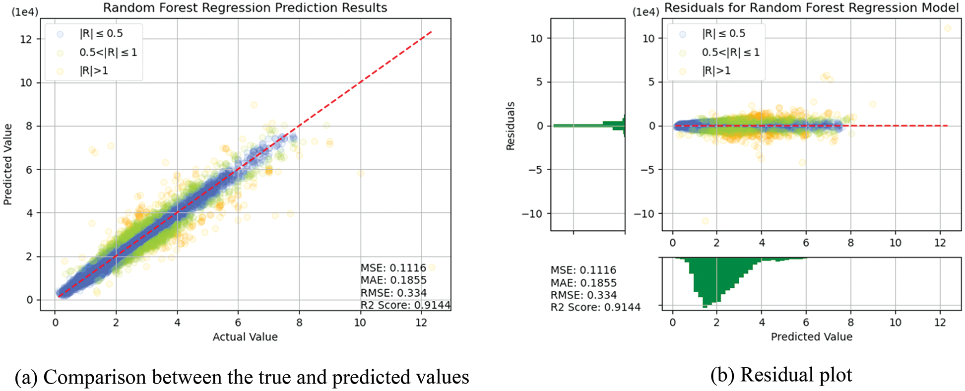
Figure 16: Prediction results of RF

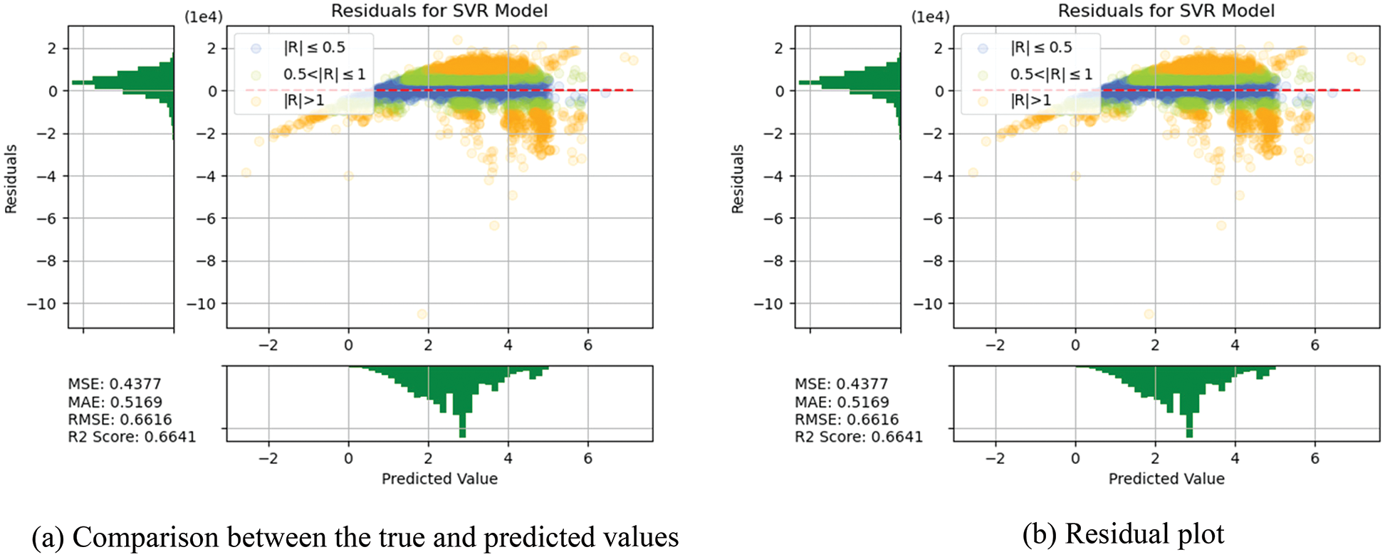
Figure 17: Prediction results of SVR

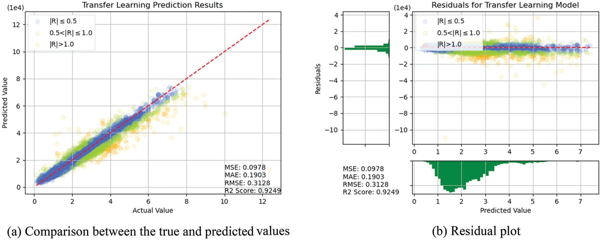
Figure 18: Prediction results of TL

5  Conclusion

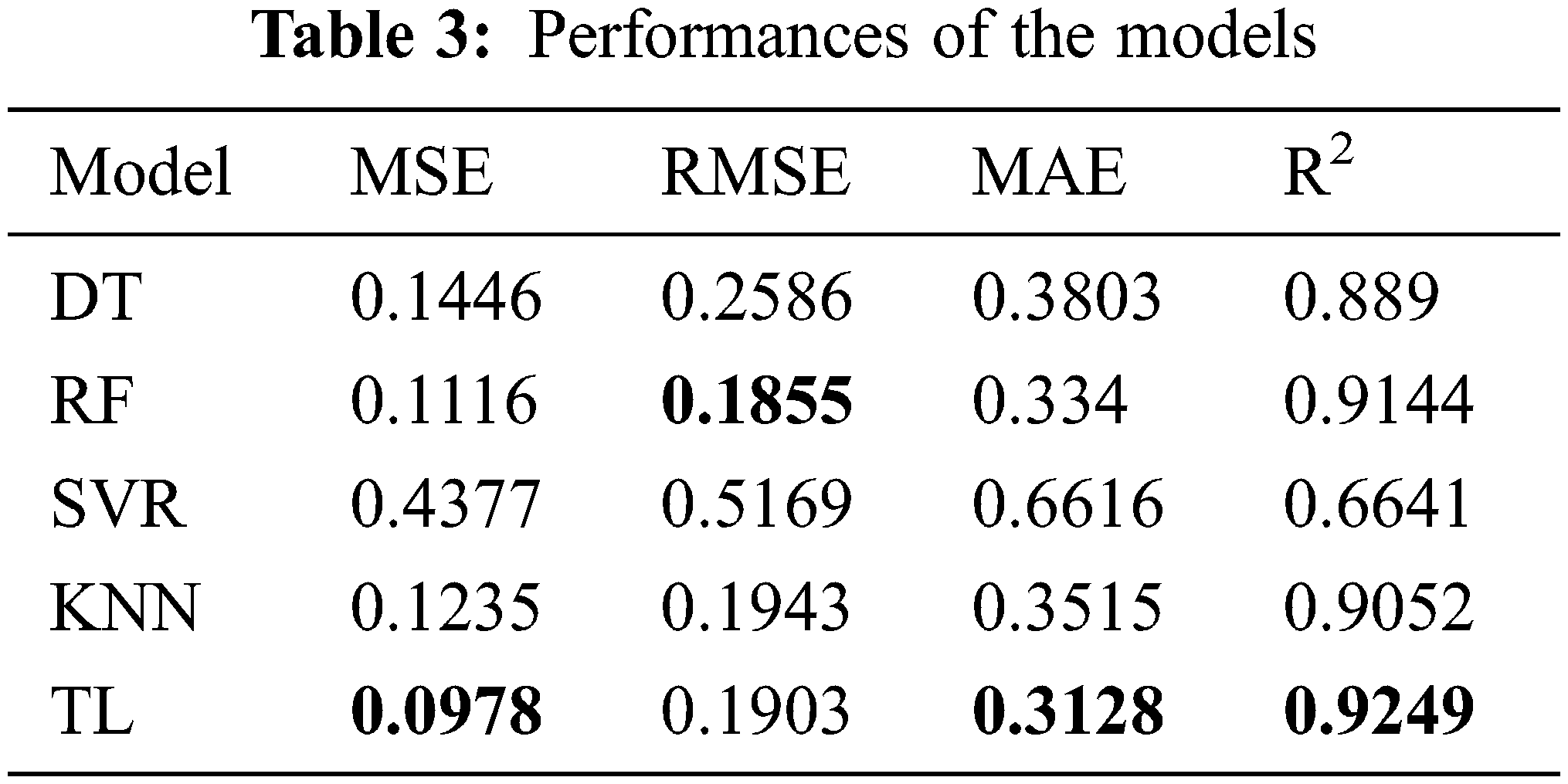
Overall, the model constructed in this study can be used to predict the selling prices of used BMW cars and is expected to be applicable in the valuation and price prediction of used cars of other brands. The model is also expected to adapt to other methods through iterations and improvements. Several parameters were used for cross-validation to facilitate training and prediction and select the most optimal model. From SVR, KNN, RF and DT basic models, we see that RF and KNN are two basic models that can provide the highest accuracy. Therefore, both models were combined with MLP in which, the fuzzy and the optical algorithms were added to carry out the TL training. The model obtained was more satisfactory than other models in terms of MSE, RMSE, and R2. Compared with a single model, TL can more effectively improve the levels of accuracy and achieve the desired training results. In the future, it is hoped that the models used in this research can help the consumers wishing to buy used cars predict the price of the used car quickly and accurately. Before using the models developed for this experiment, therefore, the data of the used cars in the respective market should be retrieved for conducting the training beforehand. The larger the data, the higher the model accuracy.

Funding Statement: This work was supported by the Ministry of Science and Technology, Taiwan, under Grants MOST 111-2218-E-194-007.

Conflicts of Interest: The authors declare that they have no conflicts of interest to report regarding the present study.

References

    1. P. Nousi, A. Tsantekidis, N. Passalis, A. Ntakaris, J. Kanniainen et al., “Machine learning for forecasting Mid-price movements using limit order book data,” IEEE Access, vol. 7, pp. 64722–64736, 2019. [Google Scholar]

    2. F. Alrowais, S. Althahabi, S. S. Alotaibi, A. Mohamed, M. Ahmed Hamza et al., “Automated machine learning enabled cybersecurity threat detection in internet of things environment,” Comput. Syst. Sci. Eng., vol. 45, no. 1, pp. 687–700, 2023. [Google Scholar]

    3. M. Valavan and S. Rita, “Predictive-analysis-based machine learning model for fraud detection with boosting classifiers,” Comput. Syst. Sci. Eng., vol. 45, no. 1, pp. 231–245, 2023. [Google Scholar]

    4. R. Punithavathi, S. Thenmozhi, R. Jothilakshmi, V. Ellappan and I. Md Tahzib Ul, “Suicide ideation detection of covid patients using machine learning algorithm,” Comput. Syst. Sci. Eng., vol. 45, no. 1, pp. 247–261, 2023. [Google Scholar]

    5. W. Cao, J. Zhang, C. Cai, Q. Chen, Y. Zhao et al., “CNN-based intelligent safety surveillance in green IoT applications,” China Commun., vol. 18, no. 1, pp. 108–119, 2021. [Google Scholar]

    6. W. Wang, Z. Wang, Z. Zhou, H. Deng, W. Zhao et al., “Anomaly detection of industrial control systems based on transfer learning,” Tsinghua Sci. Technol., vol. 26, no. 6, pp. 821–832, 2021. [Google Scholar]

    7. F. Zhuang, Z. Qi, K. Duan, D. Xi, Y. Zhu et al., “A comprehensive survey on transfer learning,” arXiv preprint, arXiv:1911.02685, 2020. [Google Scholar]

    8. M. AlDuhayyim, A. A. Malibari, S. Dhahbi, M. K. Nour, I. Al-Turaiki et al., “Sailfish optimization with deep learning based oral cancer classification model,” Comput. Syst. Sci. Eng., vol. 45, no. 1, pp. 753–767, 2023. [Google Scholar]

    9. E. Alabdulkreem, S. S. Alotaibi, M. Alamgeer, R. Marzouk, A. Mustafa Hila et al., “Intelligent cybersecurity classification using chaos game optimization with deep learning model,” Comput. Syst. Sci. Eng., vol. 45, no. 1, pp. 971–983, 2023. [Google Scholar]

  10. J. Pan, X. Wang, Y. Cheng and Q. Yu, “Multisource transfer double DQN based on actor learning,” IEEE Trans. Neural Networks Learn. Syst., vol. 29, no. 6, pp. 2227–2238, 2018. [Google Scholar]

  11. H. Takci and S. Yesilyurt, “Diagnosing autism spectrum disorder using machine learning techniques,” in 2021 6th Int. Conf. on Computer Science and Engineering (UBMK), Ankara, Turkey, pp. 276–280, 2021. [Google Scholar]

  12. L. Lu, Y. Yi, F. Huang, K. Wang and Q. Wang, “Integrating local CNN and global CNN for script identification in natural scene images,” IEEE Access, vol. 7, pp. 52669–52679, 2019. [Google Scholar]

  13. G. Shu, W. Liu, X. Zheng and J. Li, “IF-CNN: Image-aware inference framework for CNN with the collaboration of mobile devices and cloud,” IEEE Access, vol. 6, pp. 68621–68633, 2018. [Google Scholar]

  14. D. Kollias and S. Zafeiriou, “Exploiting multi-CNN features in CNN-RNN based dimensional emotion recognition on the OMG in-the-wild dataset,” IEEE Trans. Affect. Comput., vol. 12, no. 3, pp. 595–606, 2021. [Google Scholar]

  15. S. K. Roy, G. Krishna, S. R. Dubey and B. B. Chaudhuri, “HybridSN: Exploring 3-D–2-D CNN feature hierarchy for hyperspectral image classification,” IEEE Geosci. Remote Sens. Lett., vol. 17, no. 2, pp. 277–281, 2020. [Google Scholar]

  16. C. Yan, X. Wang, X. Liu, W. Liu and J. Liu, “Research on the UBI Car insurance rate determination model based on the CNN-HVSVM algorithm,” IEEE Access, vol. 8, pp. 160762–160773, 2020. [Google Scholar]

  17. 100,000 UK Used Car Data set, 2020. [Online]. Available: https://www.kaggle.com/datasets/adityadesai13/used-car-dataset-ford-and-mercedes?select = bmw.csv. [Google Scholar]

  18. Directorate General of Highways. 2021. [Online]. Available: https://www.thb.gov.tw/. [Google Scholar]

  19. M. Jeong, J. Nam and B. C. Ko, “Lightweight multilayer random forests for monitoring driver emotional status,” IEEE Access, vol. 8, pp. 60344–60354, 2020. [Google Scholar]

  20. S. Zhang, X. Li, M. Zong, X. Zhu and R. Wang, “Efficient kNN classification with different numbers of nearest neighbors,” IEEE Trans. Neural Networks Learn. Syst., vol. 29, no. 5, pp. 1774–1785, 2018. [Google Scholar]

  21. Y. Xi and H. Peng, “MLP training in a self-organizing state space model using unscented kalman particle filter,” J. Syst. Eng. Electron, vol. 24, no. 1, pp. 141–146, 2013. [Google Scholar]

  22. S. G. K. Patro and K. K. Sahu, “Normalization: A preprocessing stage,” arXiv Preprint, arXiv:1503.06462, 2015. [Google Scholar]

  23. Y. Li, M. Dong and R. Kothari, “Classifiability-based omnivariate decision trees,” IEEE Trans. Neural Networks, vol. 16, no. 6, pp. 1547–1560, 2005. [Google Scholar]

  24. A. G. Abo-Khalil and D. -C. Lee, “MPPT control of wind generation systems based on estimated wind speed using SVR,” IEEE Trans. Ind. Electron, vol. 55, no. 3, pp. 1489–1490, 2008. [Google Scholar]

  25. S. Mirjalili, S. M. Mirjalili and A. Lewis, “Grey wolf optimizer,” Adv. Eng. Softw., vol. 69, pp. 46–61, 2014. [Google Scholar]

  26. H. -C. Tsai, “Predicting strengths of concrete-type specimens using hybrid multilayer perceptrons with center-unified particle swarm optimization,” Expert Syst. Appl., vol. 37, no. 2, pp. 1104–1112, 2010. [Google Scholar]

  27. C. Luo, Y. Guo, Y. Ma, C. Lv and Y. Zhang, “A non-random multi-objective cat swarm optimization algorithm based on CAT MAP,” in 2016 Int. Conf. on Machine Learning and Cybernetics (ICMLC), Jeju Island, South Korea, pp. 29–35, 2016. [Google Scholar]

  28. J. L. Fernandez-Martinez and E. Garcia-Gonzalo, “Stochastic stability analysis of the linear continuous and discrete PSO models,” IEEE Trans. Evol. Comput., vol. 15, no. 3, pp. 405–423, 2011. [Google Scholar]

  29. S. C. Chu and P. Tsai, “Computational intelligence based on the behavior of cats,” International Journal of Innovative Computing, Information & Control, vol. 3, pp. 163–173, 2007. [Google Scholar]

Appendix

Decision Tree

As shown in Fig. 19, a DT consists of a decision diagram and a possible result. It is a type of supervised learning that can be used for classification and regression problems because it can make decisions based on data characteristics and classification categories. This means that DTs exhibit superior performance in classification tasks. However, this study focused on a regression problem, and the data exhibited no clear attribute of classification. Here, n features were assumed to exist, and each feature was assumed to represent a value. All features were then used during training until the minimum loss function was obtained. The decision-making model was as follows:

fm(x):xj+bm>0 (18)

where bm is a constant. This equation defines a hyperplane xj = bm ­orthogonal to the xj axis and divides the input space into two parts.

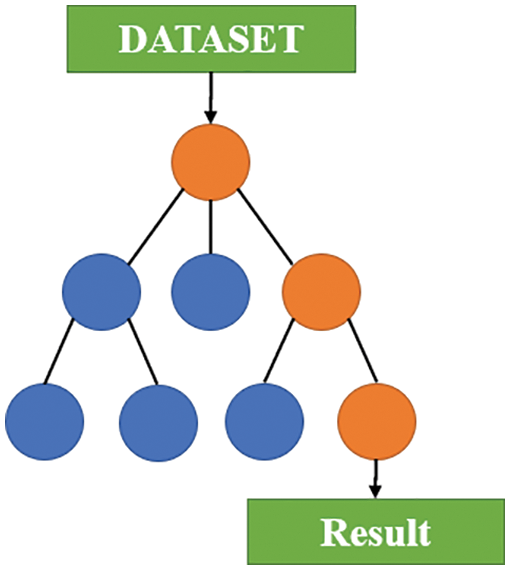
Figure 19: Structure of a DT

Random Forest

RF is a type of combination algorithm based on DTs, as shown in Fig. 20. It is composed of multiple DTs and is an overall learning algorithm created using bagging and random feature sampling. Compared with DTs, RF is less prone to overfitting and can more effectively deal with classification and regression problems. For most types of data, the fitting results of RF are highly accurate. However, RF requires a large memory during operation to store the data of each DT. In addition, because RF is a learning algorithm of a combination of DTs, it cannot provide an explain for an individual DT.

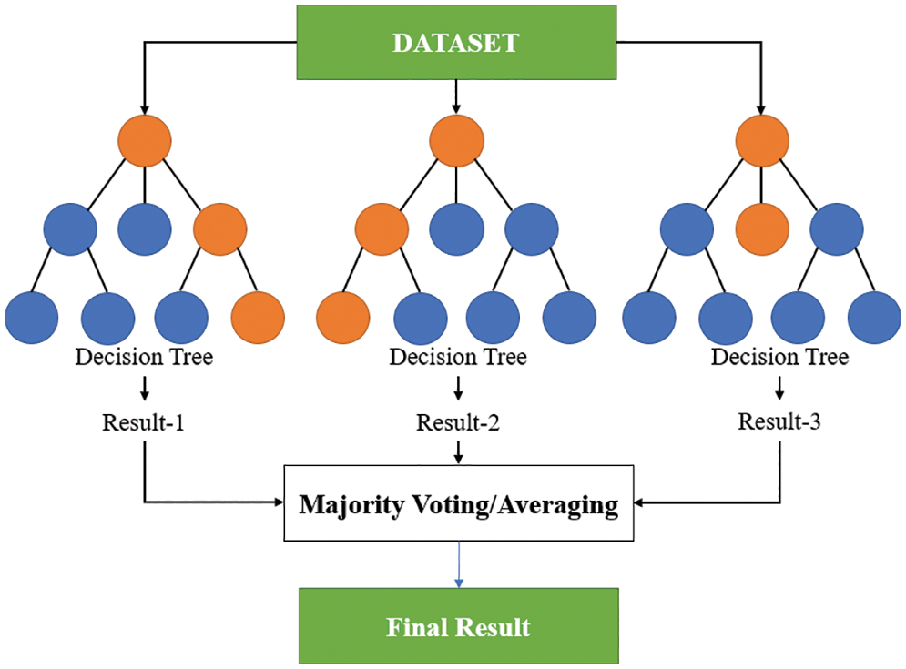
Figure 20: Schematic of RF

Support Vector Regression

SVR is an algorithm based on SVMs and is used to solve regression problems. An SVM simply adds an extra dimension to the original one to find a straight line that divides the data for classification, as shown in Fig. 21.

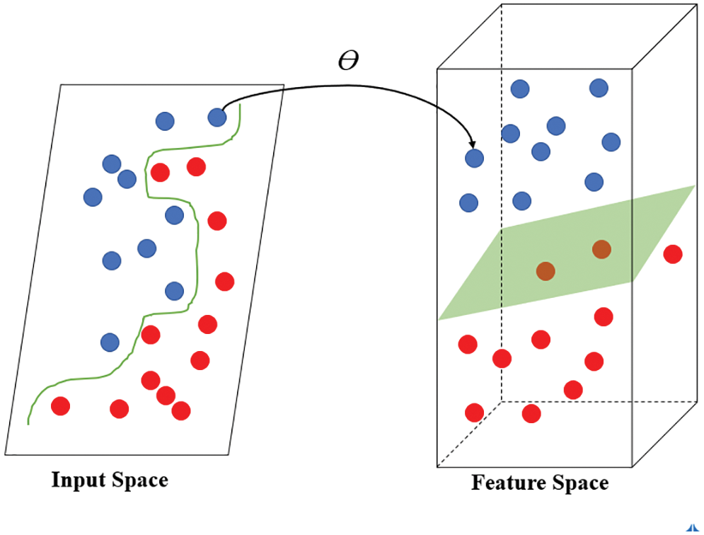
Figure 21: Schematic of an SVM

The SVM contains three essential parameters: a kernel, a hyperplane, and a decision boundary. The kernel is used to identify the hyperplane among high-level dimensions. The hyperplane is the dividing line between two data points in the SVM and is used to predict continuous output in SVR. The decision boundary is the boundary between decisions.

SVR first considers the sample points in the decision boundary and then fully utilizes these points. A schematic of SVR is presented in Fig. 22 and its relevant questions are as follows:

f(x)=(ω⋅Φ(x))+b (19)

Rreg(f)=12||ω||2+C∑i=1n⁡Γ(f(xi)−yi) (20)

|yi−ω⋅Φ(xi)−b|≤ϵ+ξi,  i=1, 2, ⋯, n  (21)

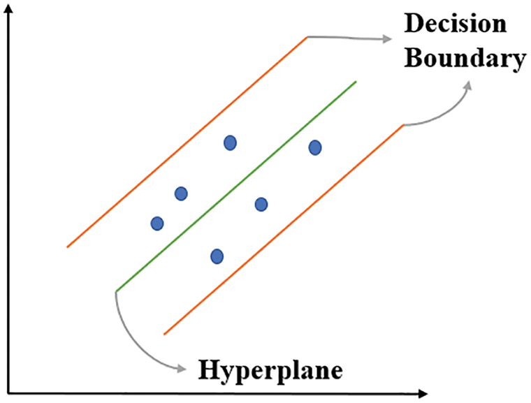
Figure 22: Schematic of SVR

where ω is the weight matrix, b is the bias term, Ф is the nonlinear transformation from an n-dimensional space to a higher-dimensional feature space, Γ is the cost function, ε is the allowable error, and C is a constant that determines the tradeoff between the minimal training error and minimal model complexity ||ω||­­2. The vectors outside the ε-tube can be obtained by using the slack variables ξi.

K-Nearest Neighbors

KNN is a simple and easy-to-use supervised algorithm. It can be used to solve classification and regression problems. However, although KNN is easy to use and understand, it has a major disadvantage: it considerably slows down when the size of the data increases. As shown in Fig. 23, KNN assumes that similar events are nearby and classifies these events accordingly.

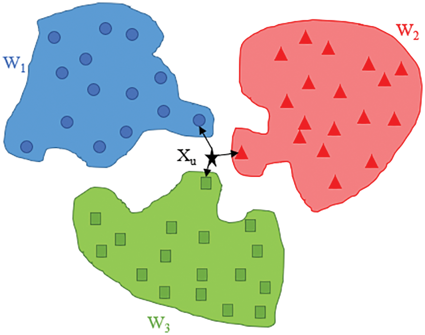
Figure 23: Schematic of KNN

The working principle of KNN is to estimate the distance between a query and all samples in the data, select the specified number of classification K that is closest to the query, and vote for the most frequent result. In regression scenarios, all results are averaged.

As shown in Fig. 23, the Xu value is closer to the members of the W3 group than to the members of the other groups. Therefore, Xu is classified as a member of the W3 group.