Harris Hawks Optimizer with Graph Convolutional Network Based Weed Detection in Precision Agriculture

1  Introduction

Weeds are unwanted plants that grow in fields and compete with crops for light, water, space, and nutrients. If uncontrollable, they might have many adverse impacts like loss of crop yields, contamination of grain during harvesting, and production of a considerable amount of seeds, thus forming a weed seed bank in the fields [1]. Conventionally, weed management program involves the control of weeds via mechanical or chemical resources, namely the uniform application of herbicides all over the fields [2]. But, the spatial density of weeds isn’t uniform throughout the fields, thus resulting in the overuse of chemicals that lead to the evolution of herbicide-resistant weeds and environmental concerns. A site-specific weed management (SSWM) concept that represents detecting weed patches and removal or spot spraying by mechanical resources was introduced to resolve these shortcomings in the early 90s [3]. Earlier control of Weeds in the season is crucial because the weed will compete with the crop yields for the resource in the development phase of the crops, which leads to potential yield loss [4–6]. A considerable study has developed specific variable spraying methods to prevent waste and herbicide residual difficulties caused by conventional full-coverage spraying [7]. To accomplish accurate variable spraying, a major problem must be resolved in real-time accurate identification and detection of weeds and crops. Approaches to realizing the weed detection field through the computer vision (CV) technique primarily involve deep learning (DL) and conventional image processing [8]. While the detection of weeds is carried out with conventional image-processing techniques, extracting features, like shape, color, and texture, of the image and combining with conventional machine learning (ML) approaches like Support Vector Machine (SVM) or random forest (RF) approach, for the detection of weeds are needed [9]. Such techniques should have high dependence and design features manually on the quality of feature extraction, pre-processing methods, and image acquisition methods. With the increase in data volume and the advancement in computing power, the DL algorithm could extract multi-dimensional and multi-scale spatial semantic features of weed via Convolution Neural Network (CNN) because of their improved data expression abilities for images, which avoids the disadvantage of conventional extraction method [10]. Consequently, they have gained considerable interest among the researcher workers.

Ukaegbu et al. [11] define the advancement of a modular unmanned aerial vehicle (UAV) to eradicate and detect weeds on farmland. Precision agriculture involves resolving the issue of poor agricultural yield because of competition for nutrients by weeds and offers a rapid method to eliminate the difficult weeds utilizing developing technologies. This work has solved the mentioned problem. A quadcopter has been built, and lightweight resources accumulate elements. The system has a lithium polymer (li-po) battery, electric motor, propellers, receiver, flight controller, electronic speed controller, GPS, and frame. In [12], a DL mechanism can be advanced to find crops and weeds in croplands. The advanced system has been enforced and assessed by high-resolution UAV images captured on 2 different target fields: strawberry and pea; the advanced system can find weeds. In [13], a method can be advanced for accelerating the manual labelling of pixels utilizing a 2-step process. Firstly, the foreground and background were divided by maximum likelihood classification; secondly, the weed pixels were labelled manually. These labelled data were utilized for training semantic segmentation techniques that classify crop and background pixels into one class and other vegetation into the second class.

Osorio et al. [14] devise 3 techniques for weed estimation related to DL image processing in lettuce crops and a comparison made to visual assessments by professionals. One technique depended on SVM utilizing histograms of oriented gradients (HOG) as feature descriptors. The second one depends on YOLOV3 (you only look once at V3), using its robust structure for object detection. The last method relies upon Mask R-CNN (region-oriented CNN) to receive an instance segmentation for every individual. Such techniques are supplemented with a normalized difference vegetation index (NDVI) index (normal difference vegetation indexes) as a background sub-tractor to remove non-photosynthetic objects. In [15], a novel technique that integrates high-resolution RGB and low-resolution MS imageries is presented for detecting Gramineae weed in rice fields with plants 50 days afterwards emergence. The images were taken from a UAV. The presented technique will combine the texture data offered by high-resolution RGB imagery and the reflectance data presented by low-resolution MS imagery to obtain an integrated RGB-MS image with superior weed-discriminating features. After scrutinizing the normalized green-red difference index (NGRDI) and NDVI for detecting weeds, it is noted that NGRDI provides superior features.

This study presents a Harris Hawks Optimizer with Graph Convolutional Network based Weed Detection (HHOGCN-WD) technique for Precision Agriculture. The presented HHOGCN-WD technique mainly focuses on identifying and classifying weeds for precision agriculture. For image pre-processing, the HHOGCN-WD model utilizes a normal bilateral filter (BNF) for noise removal. In addition, coupled convolutional neural network (CCNet) model is utilized to derive a set of feature vectors. To detect and classify weed, the GCN model is utilized with the HHO algorithm as a hyperparameter optimizer to improve the detection performance. The experimental results of the HHOGCN-WD technique are investigated under the benchmark dataset.

2  The Proposed Model

This study developed a new HHOGCN-WD technique for weed detection and classification for Precision Agriculture. The presented HHOGCN-WD technique mainly focuses on identifying and classifying weeds for precision agriculture. Fig. 1 depicts the overall block diagram of the HHOGCN-WD approach.

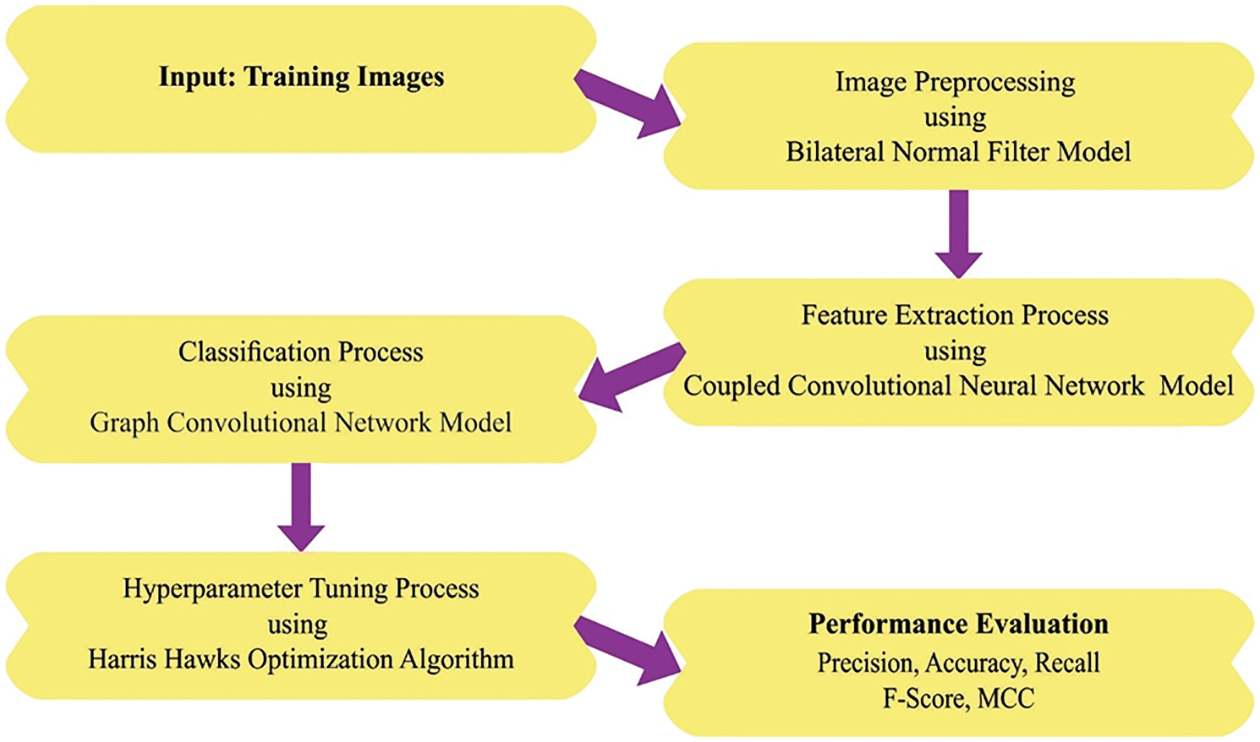
Figure 1: Overall block diagram of HHOGCN-WD approach

2.1 Image Pre-Processing

For image pre-processing, the HHOGCN-WD model utilizes BNF for noise removal. The BNF technique is a two-stage process that upgrades normal Niter time and later upgrades vertices Viter times [16]. The procedure of denoising process with the BNF is denoted by (update normal)  Niter + (update vertices)  Viter . The BNF upgrades the normal vector through the weighted average of the noisy neighbourhood normal vector in the following [16]:

n~i=1Ki×∑fjϵϕi ⁡AjWC(‖c(fi) −c(fj)‖,  σc)WS(‖ni−nj‖,  σs)nj (1)

In Eq. (1), Ki denotes the normalization factor. σc and σs control the kernel width of Gaussian function WC and WS , correspondingly [16],

WC(‖c(fi)−c(fj)‖,  σc)= exp (−‖c(fi)−c(fj)‖22σc2),  (2)

WS(‖ni−nj‖,  σs)= exp (−‖ni−nj‖22σs2). (3)

Function WC provides a smaller weight while the distance between the geometric center (the centroids) of  fi and the adjacent face is larger. Function WS provides additional weight as a similarity between neighbouring normal and ni rises.

2.2 Feature Extraction: CCNet Model

The CCNet model is utilized at this stage to derive a set of feature vectors. It is well-known that CNN has established impressive abilities in image processing. Likewise, numerous CNN and derivative has been proposed for capturing the neighbourhood spatial feature from the image in weed classification [17]. The discriminatory feature allows discrimination against targeted regions in complicated scenes.

It is noted that the input dataset ( XH or XL) is initially transported to the adjacency patch sampler that samples and produces a sequence of adjacency patches (3D spectral cubes PH∈Rp×p×D or 2D elevation path PL∈Rp×p) from the novel dataset based on the provided neighborhood size (p×p) . Then, they are fed into the respective CNN module for representation learning or feature extraction. Especially the model primarily comprises two nearly similar CNN architectures for LiDAR and HS datasets, correspondingly. The input to the CNN at the top of the figure is PH extracted from the hyperspectral images, whereas the input to the CNN at the bottom is PL extracted from the LiDAR images. It should be noticeable that the two used CNN network contains 4 convolution blocks. Those blocks have the same architecture comprising nonlinear activation, convolution, batch normalization (BN), and MaxPooling layers. For all the CNN networks, the amount of convolution kernels in four convolution layers is 32, 64, 128, and 128, correspondingly. The initial 3 convolution layer uses a size of 3×3  convolution kernel, and the final layer is 1×1 . CH∈RN×128 and CL∈RN×128 represent the short-range spatial feature extracted from the CNN on LiDAR and HS dataset, correspondingly.

Because of the weight-sharing module, the two CNN networks share the parameter and setting of the additional 3 convolution layers, excluding the initial convolution layer. It has the apparent advantage of a larger reduction in several major variables. Then, the convolutional operation rule of the two CNN models is shown below:

Hjl+1=f(∑m ⁡HmlWj,ml+1+bj,ml+1). (4)

In Eq. (4), Hml indicates the mth feature maps at the lth layers. Wj,ml+1 signifies the jth convolutional kernel interconnected with the mth feature map at (l+1)th layers, and bj,ml+1 indicates the corresponding bias. Now, H0=PH or PL.f(.) represents the nonlinear activation functions such as ReLU. The size of the sampled neighborhood could considerably affect the concluding classifier outcome.

2.3 Weed Detection Using GCN Model

This study utilises the GCN model to detect and classify weeds. Assume an input image I, the objective of multilabel image classifier is to evaluate a f function which forecasts the occurrence or not of label belonging to a set ℒ={1,  N} , and it is formulated in the following [18],

f:Rw×h→[0, 1]N

I↦y=(yi)i∈ℒ, 

where w and h correspondingly represent the pixel-wise width and height of the image. Noted that yi=1 when the label i exists in I or yi=0 . As deliberated in Section 1, graph-based multi-label models, namely IML-GCN and ML-GCN, comprise two subdivisions. The initial one depends on the out-off-shelf CNN models, which allow the extraction of discriminatory image representation. Especially, IML-GCN and ML-GCN integrate a TResNet-M and ResNet-101. The latter comprises an effective form of ResNet-50. The next branch depends on a specific GCN aim is to generate N inter-dependent binary classifications. Consider the input graph = {V,  E,  F} , with V = [v1,  v2, …,  vN] the subset of vertices so that vi corresponding to the vertex related to the label, E=[e1,  e2,  …,  eM] the subset generated using M edges interconnecting the vertices and F=[f1,  f2,  fN] the vertex features so that fi∈Rd characterizes the feature of vertex i. Consider A∈RN×N as the neighborhood matrix defining the topology of the graph. A is evaluated by assuming the co -occurrence possibility of the label. Additionally, a threshold τ is fixed and is utilized for ignoring rare co -occurrence that is regarded as noisy. For i, j∈ℒ,

Aij={0,  if Pij<T, 1,  if Pij≥T ′ (5)

In Eq. (5), Pij=P(j|i) indicates the co -occurrence probability that the label j seems provided that i is previously presented.

Next, assume that Fl∈Rn×dl encoded the input vertex feature of lth layer, the GCN calculates the node feature of (l+1)th layer Fl+1∈Rn×dl+1 ,

Fl+1=h(AFlWl). (6)

where h refers to the nonlinear activation function frequently selected as a Leaky Rectified Linear Unit (Leaky ReLU), Wl∈Rdl×dl+1 the learned weight matrixes of layer l. Noted that A is standardized beforehand employing the above equation. Lastly, the vertex feature is generated using the final layer from the N inter-dependent classifier.

2.4 Hyperparameter Tuning

This study applies the HHO algorithm as a hyperparameter optimizer to improve detection performance. The HHO technique utilized 2 distinct approaches to searching functions from the exploration stage [19]. Each of the approaches is chosen dependent upon q; If q≥0.5 , a direct approach has been utilized for searching nearby most other hawks arbitrarily. However, if q<0.5 , the second approach has been utilized for the searching function formulated in Eq. (7) [19].

X(t+1)={Xrand(t)−r1|Xrand(t)−2r2X(t)|q≥0.5(Xrabbit(t)−Xm(t))−r3(LB+r4(UB−LB))q<0.5.  (7)

whereas Xm(t) is computed dependent upon Eq. (8).

Xm(t)=1N∑i=1N⁡Xi(t).  (8)

A distinct process was utilized for moving from the exploration to the exploitation stages. In optimized functions, the exploration function was carried out first, then the exploitation function, by improving the iterations, defining an optimum solution, and creating a promising solution. Eq. (9) has been utilized for mathematical modeling.

E=2E0(1−tT).  (9)

If |E|≥1 , this technique enters the exploration stage. However, if |E|<1 , it enters the exploitation stage. The value of E is a reducing movement in the maximum of iterations. The HHO technique utilizes 4 distinct approaches for carrying out optimized functions from the exploitation stage. If E≥ 0.5 , 2 approaches were employed, such as besiege and soft besiege with advanced rapid dives. On the contrary, if E<0.5 , 2 approaches like besiege and hard besiege with advanced rapid dives were utilized. All of these approaches are described under.

Soft besiege

If r≥0.5 and |E|≥0.5 , the HHO technique employs a soft besiege technique to optimize functions. During this case, hawks could not simply hunt rabbits as has a lot of energy for escaping, as determined in Eqs. (10) and (11).

X(t+1)=ΔX(t)−E|JXrabbit(t)−X(t)|.  (10)

ΔX(t)=Xrabbit(t)−X(t).  (11)

In Eq. (10), ΔX , achieved utilizing in Eq. (11), signifies the distance of chosen hawk to a rabbit, and E has been attained utilizing in Eq. (14). J is also escaping the energy of rabbits, which is achieved by utilizing Eq. J=2(1−r5) .

Hard besiege

If r≥0.5 and |E|<0.5 , the HHO approach utilizes a hard besiege method to optimize functions. During this work, the hawks hunt rabbits with a rapid attack as it no longer has sufficient energy to escape. The mathematical process of this motion was formulated utilizing Eq. (12).

X(t+1)=Xrabbit(t)−E|ΔX(t)|.  (12)

If |E|≥0.5 but r <0.5 , the soft besiege technique with progressive rapid dives has been utilized. Then, the rabbit is sufficient energy to escape, and there is until a soft besiege. This process was comparatively more advanced than the earlier process.

Y=Xrabbit(t)−E|JXrabbit(t)−X(t)|.  (13)

This method utilizes a Lévy flight (LF) to improve efficiency. In addition, the 2 states of Eq. (18) were related to the present solution. The LF could not be utilized as an outcome of Y but is employed in Z, provided in Eq. (8).

Z=Y+S×LF(D).  (14)

In Eq. (14), S refers to the arbitrary number from the dimension of problems from the range of zero and one, and LF(D) refers to the LF from the dimensional of problems demonstrated in Eq. (15).

LF(x)=0.01×u×σ|v|1β, σ=(r(1+β2)×β×2(β−12)Γ(1+β)×sin⁡(πβ2))1β.  (15)

In Eq. (15), u and v represent the 2 arbitrary numbers between zero and one, and β has a set and default number, that is, 1.5.

X(t+1)={Y if F(Y)<F(X(t))Z if F(Z)<F(X(t)).  (16)

Based on Eq. (16), the outcome of Eq. (13) is superior to the present solutions and, therefore, changes it; else, the solution achieved in Eq. (14) is related to the present solutions. Assume that |E|<0.5 and r<0.5 , the hard besiege approach with advanced rapid dives has been utilized to optimize functions. Then, the rabbit could not have sufficient energy to escape and was besieged hard before the surprise pounced to catch the rabbit. Eqs. (18) and (19) execute dependent upon Eq. (17).

X(t+1)={Y if F(Y)<F(X(t))Z if F(Z)<F(X(t)).  (17)

In Eq. (17), Y and Z are attained utilizing Eqs. (18) and (19).

Y=Xrabbit(t)−E|JXrabbit(t)−Xm(t)|.  (18)

Z=Y+S×LF(D).  (19)

During this approach, the solution achieved in Eq. (18) changes the present solution when it can be more effective than others; else, the solution achieved in Eq. (19) is exchanged when it can be more effective than the present solution. Fig. 2 showcases the flowchart of the HHO technique.

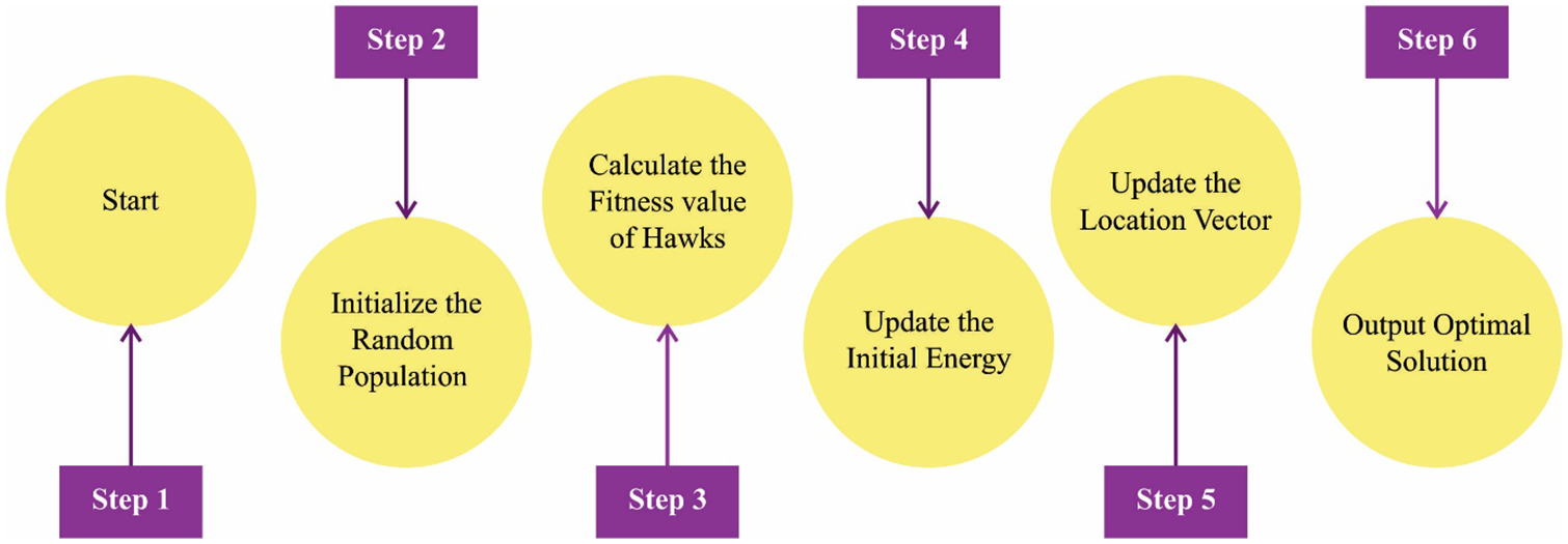
Figure 2: Flowchart of HHO technique

3  Results and Discussion

The weed detection performance of the HHOGCN-WD model is tested using a benchmark weed dataset [20]. The dataset holds 3000 samples with two classes, as in Table 1. A few sample images are demonstrated in Fig. 3.

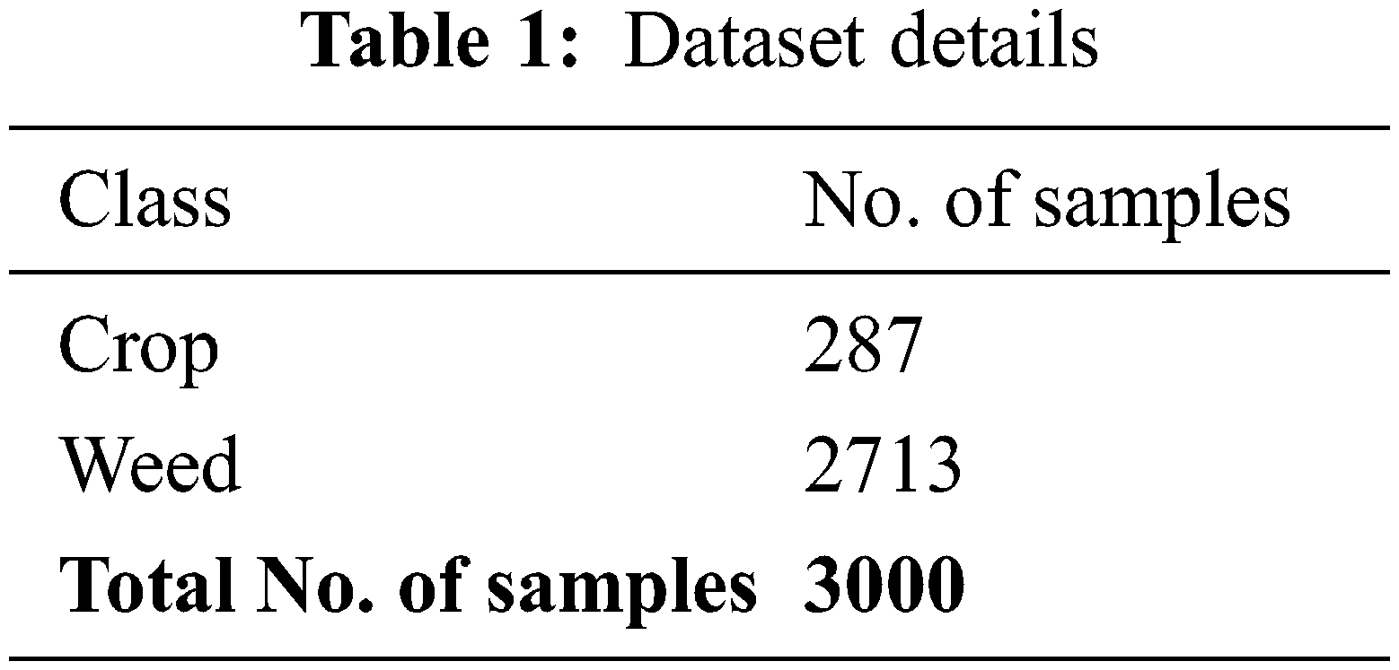
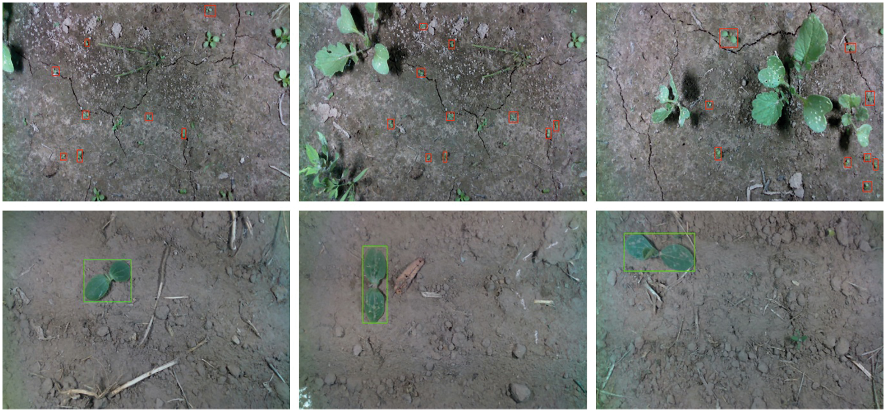
Figure 3: Sample images

Fig. 4 depicts the confusion matrices offered by the HHOGCN-WD model under five distinct runs. The figure implied that the HHOGCN-WD model had identified the weeds proficiently under each class. For instance, on run-1, the HHOGCN-WD model detected 274 samples under crop and 2693 samples under weed class. Moreover, on run-2, the HHOGCN-WD technique detected 278 samples under crop and 2692 samples under weed class. Further, on run-3, the HHOGCN-WD approach detected 274 samples under crop and 2693 samples under weed class. Then, on run-4, the HHOGCN-WD technique detected 270 samples under crop and 2695 samples under weed class. Next, on run-5, the HHOGCN-WD method detected 282 samples under crop and 2692 samples under weed class.

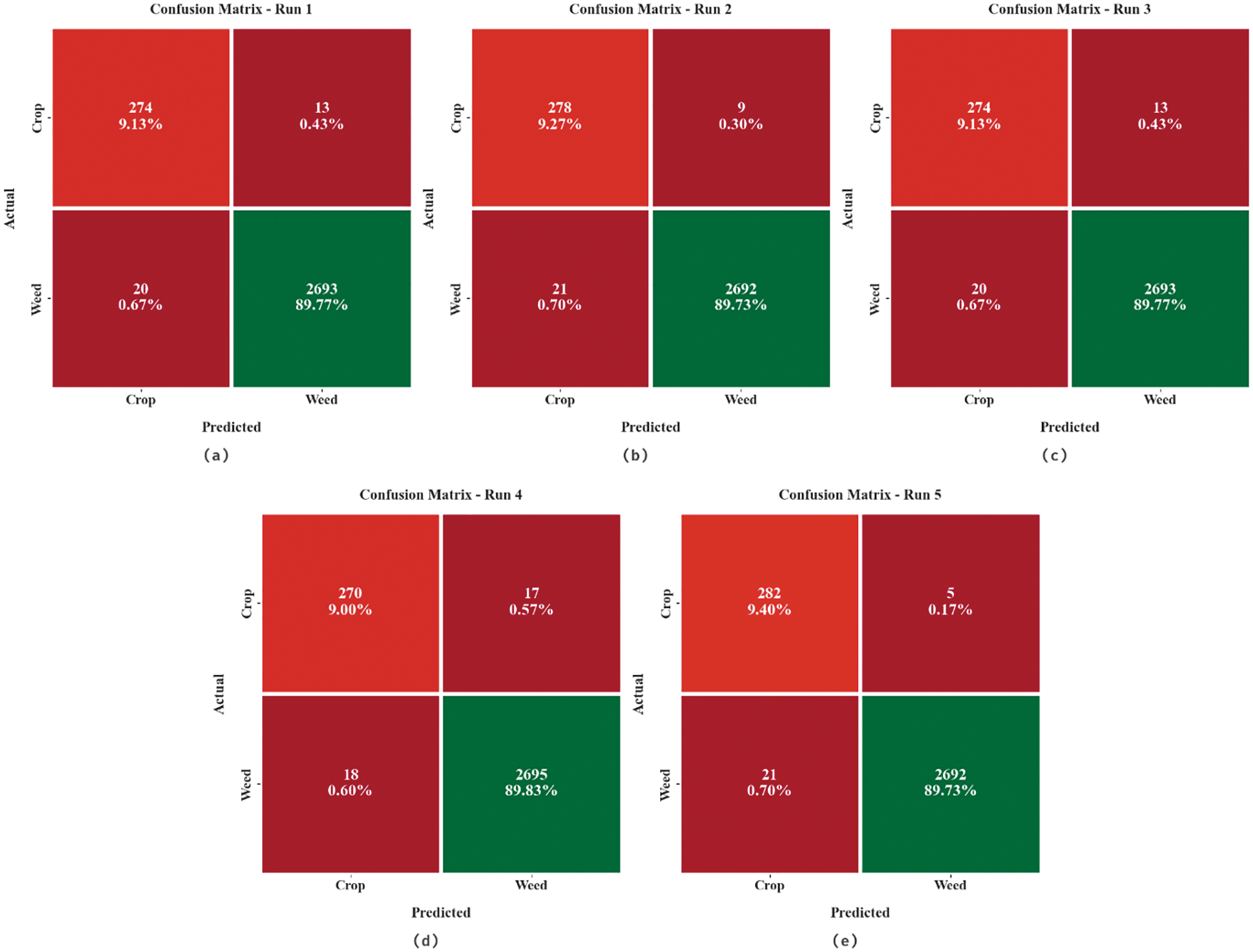
Figure 4: Confusion matrices of HHOGCN-WD approach (a) Run1, (b) Run2, (c) Run3, (d) Run4, and (e) Run5

Table 2 and Fig. 5 demonstrate the overall weed detection outcomes of the HHOGCN-WD model under five distinct runs. The results indicated that the HHOGCN-WD model had shown enhanced weed detection outcomes. For instance, on run-1, the HHOGCN-WD model has offered average accuy , precn , recal , Fscore , and MCC of 98.90%, 96.36%, 97.37%, Fscore of 96.86%, and MCC of 93.72%. In the meantime, on run-2, the HHOGCN-WD technique has rendered average accuy , precn , recal , Fscore , and MCC of 99%, 96.32%, 98.05%, Fscore of 97.16%, and MCC of 94.35%. Similarly, on run-3, the HHOGCN-WD method has presented average accuy , precn , recal , Fscore , and MCC of 98.90%, 96.36%, 97.37%, Fscore of 96.86%, and MCC of 93.72%. Additionally, on run-4, the HHOGCN-WD methodology has rendered average accuy , precn , recal , Fscore , and MCC of 98.90%, 96.56%, 96.71%, Fscore of 96.63%, and MCC of 93.27%. Finally, on run-5, the HHOGCN-WD algorithm has provided average accuy , precn , recal , Fscore , and MCC of 99.13%, 96.44%, 98.74%, Fscore of 97.56%, and MCC of 95.16%.

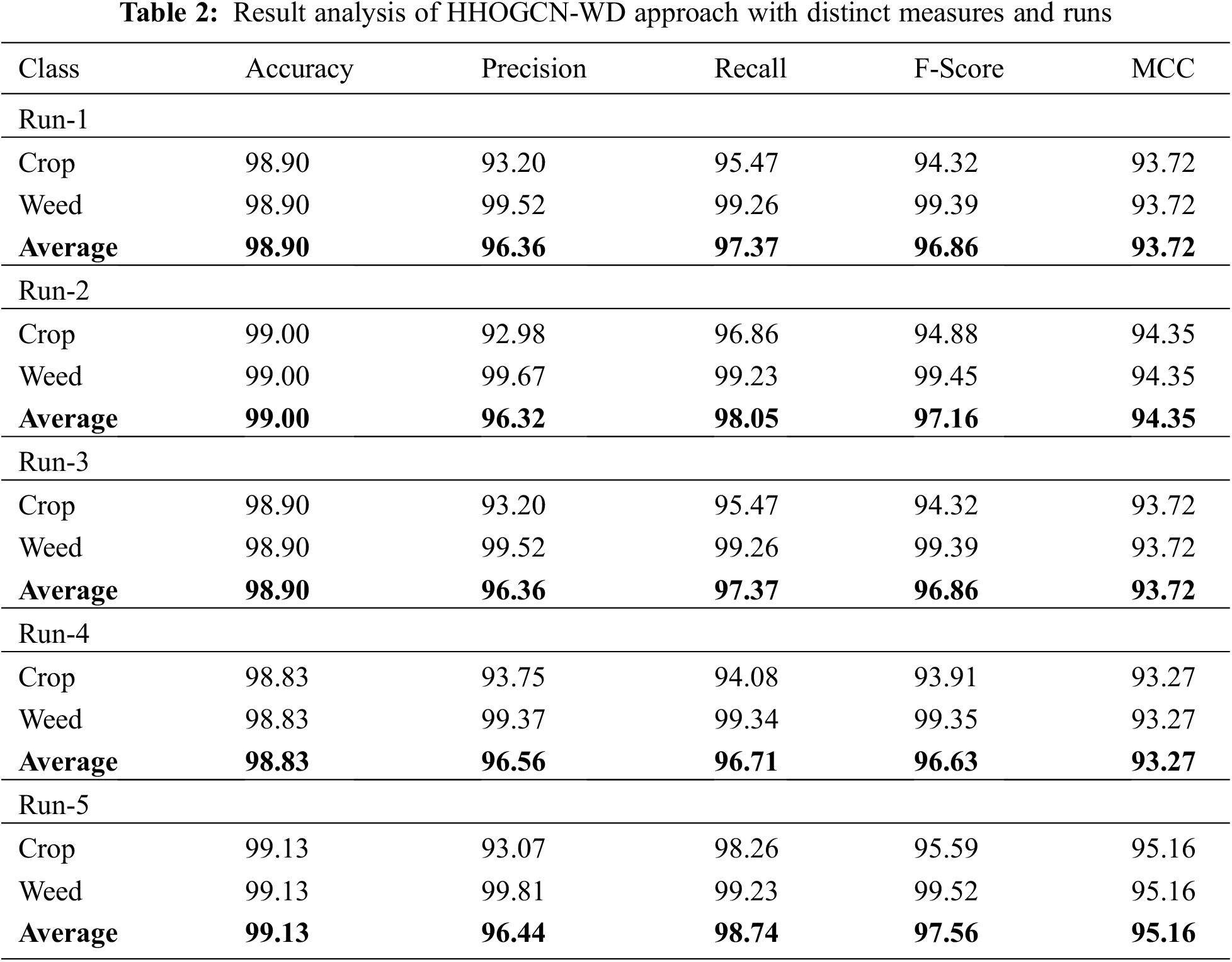
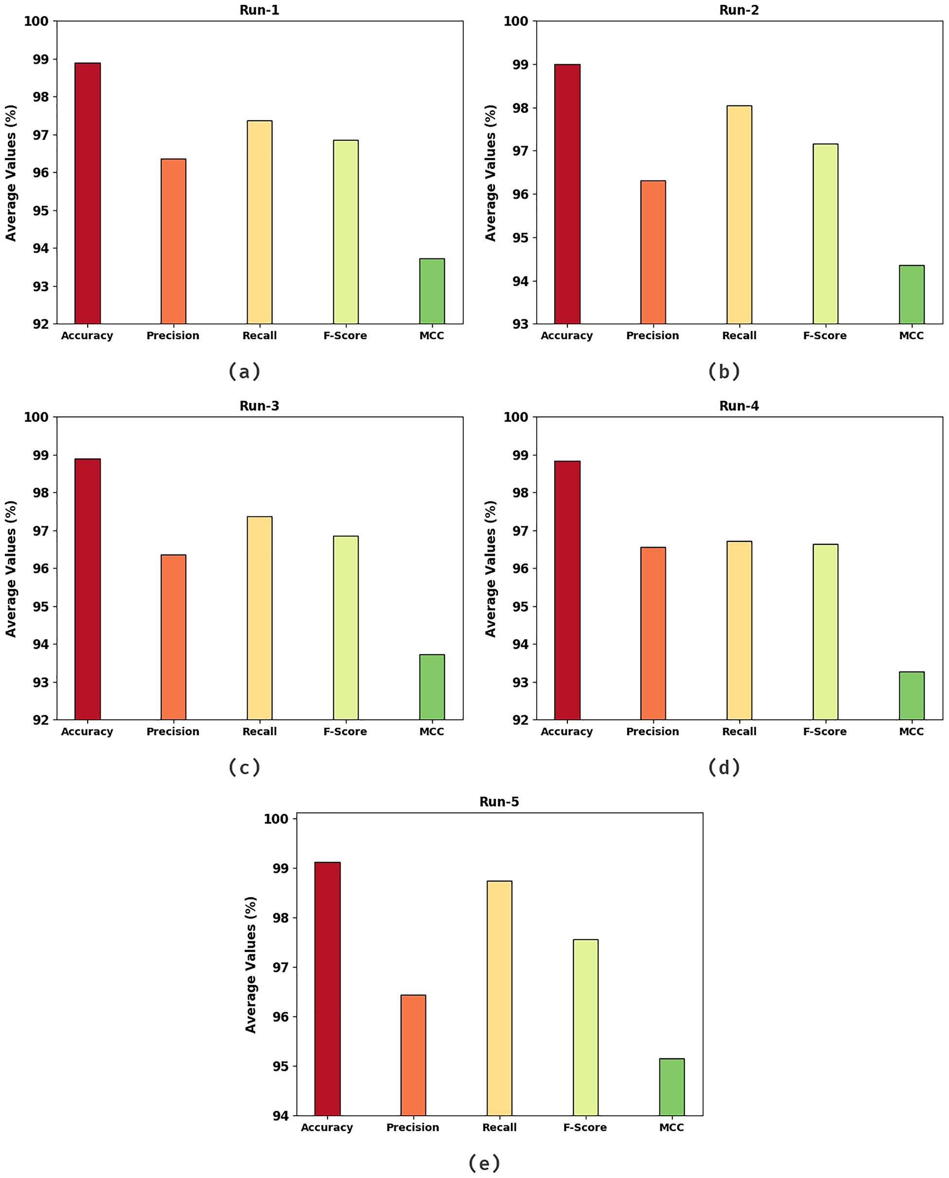
Figure 5: Average analysis of HHOGCN-WD approach (a) Run1, (b) Run2, (c) Run3, (d) Run4, and (e) Run5

The training accuracy (TRA) and validation accuracy (VLA) acquired by the HHOGCN-WD approach in the test dataset is shown in Fig. 6. The experimental outcome implicit in the HHOGCN-WD method has attained maximal values of TRA and VLA. Seemingly the VLA is greater than TRA.

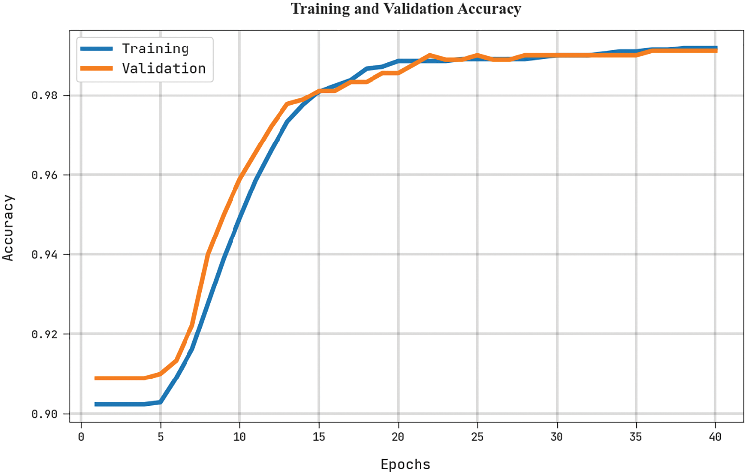
Figure 6: TRA and VLA analysis of HHOGCN-WD approach

The training loss (TRL) and validation loss (VLL) obtained by the HHOGCN-WD method in the test dataset are accomplished in Fig. 7. The experimental outcome denotes the HHOGCN-WD approach has exhibited the least values of TRL and VLL. Particularly, the VLL is lesser than TRL.

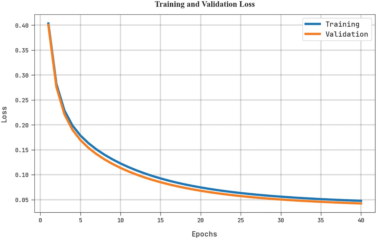
Figure 7: TRL and VLL analysis of the HHOGCN-WD approach

A clear precision-recall inspection of the HHOGCN-WD algorithm in the test dataset is given in Fig. 8. The figure representing the HHOGCN-WD approach has resulted in enhanced precision-recall values in all classes.

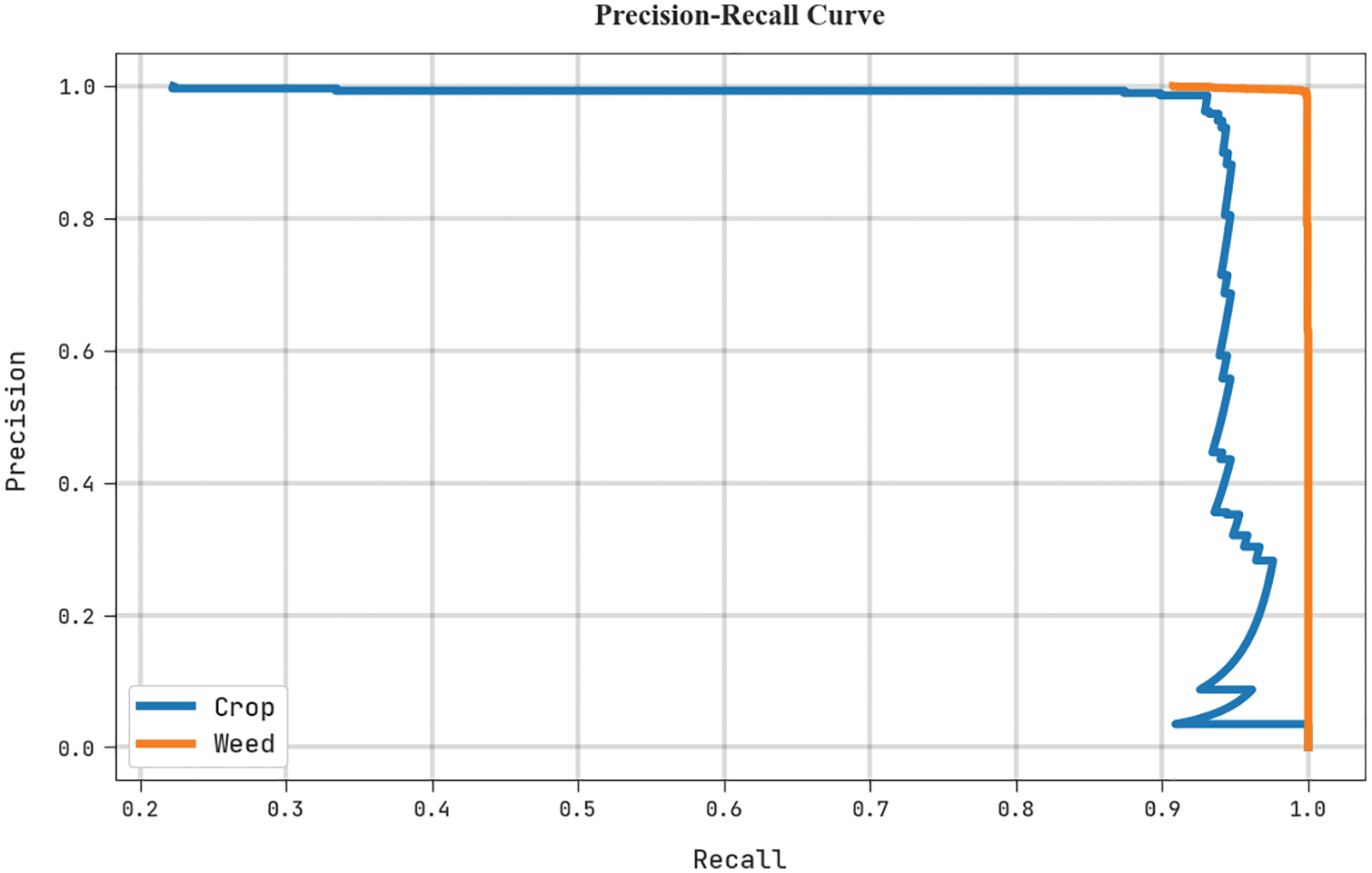
Figure 8: Precision-recall analysis of the HHOGCN-WD approach

A brief ROC investigation of the HHOGCN-WD technique under the test dataset is portrayed in Fig. 9. The results implicit the HHOGCN-WD method has displayed its ability in classifying distinct class labels in the test dataset.

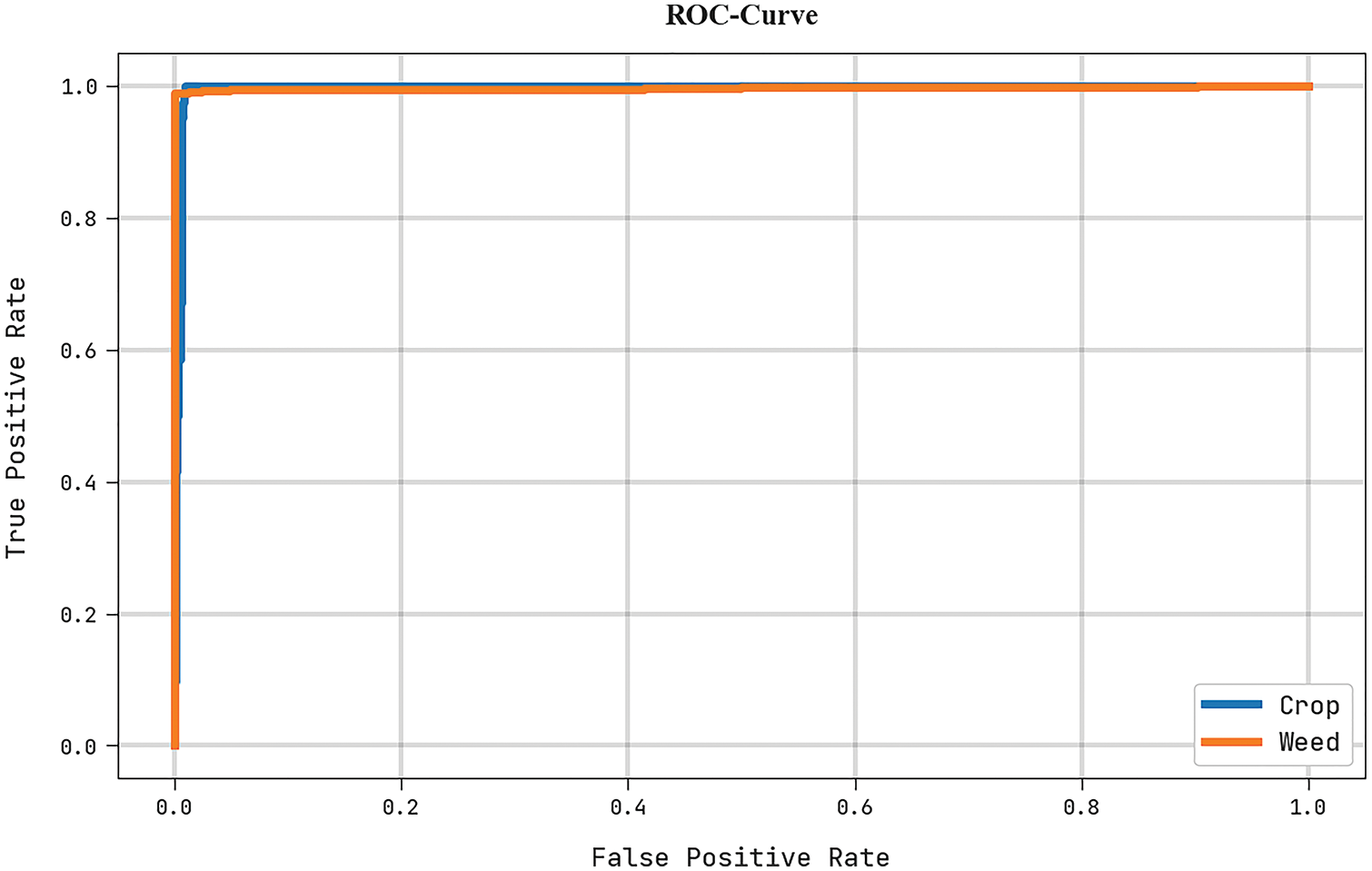
Figure 9: ROC analysis of HHOGCN-WD approach

Table 3 and Fig. 10 depict the comparison weed detection results of the HHOGCN-WD model with other existing models [21,22]. The results implied that the HHOGCN-WD model has obtained enhanced results in terms of different measures. For instance, concerning accuy , the HHOGCN-WD model has offered an increased accuy of 99.13%, whereas the AlexNet, GoogleNet, Inception v3, Mask RCNN, and CNN-WIS model have reached a reduced accuy of 96.33%, 95.38%, 97.57%, 97.49%, and 97.38% respectively. Temporarily, concerning prenc , the HHOGCN-WD algorithm has presented an increased prenc of 96.44% whereas the AlexNet, GoogleNet, Inception v3, Mask RCNN, and CNN-WIS technique have attained a reduced prenc of 95.60%, 94.50%, 95.56%, 95.86%, and 95.69% correspondingly.

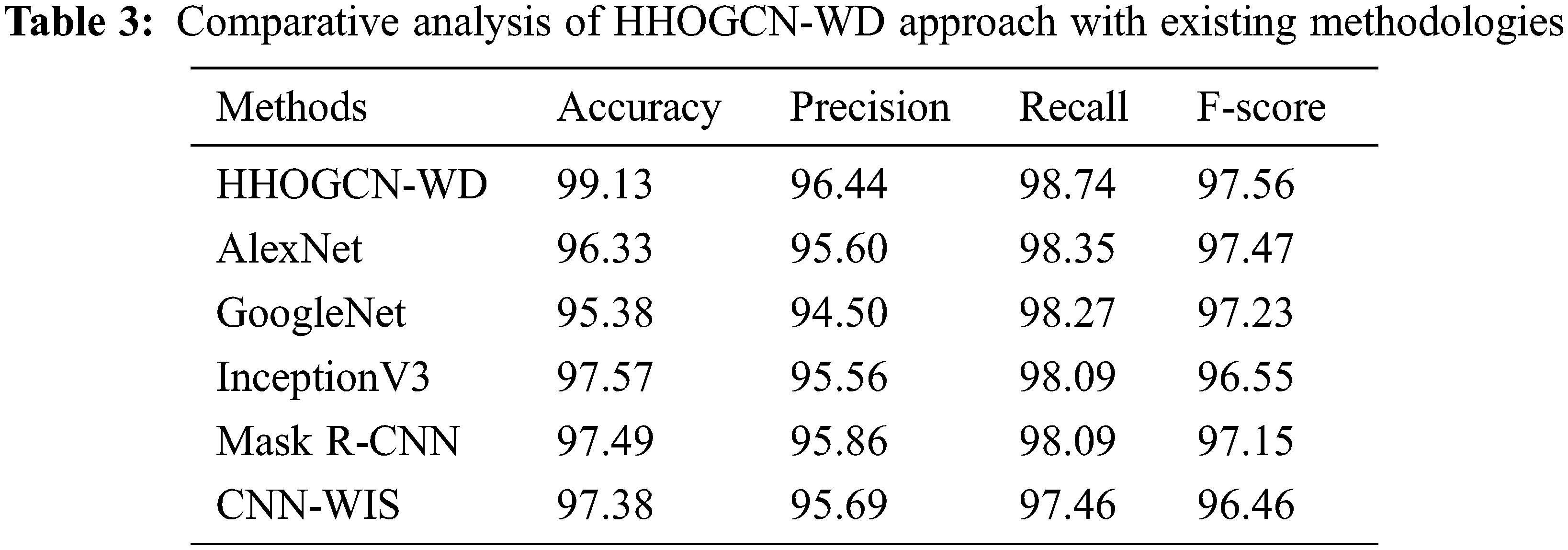
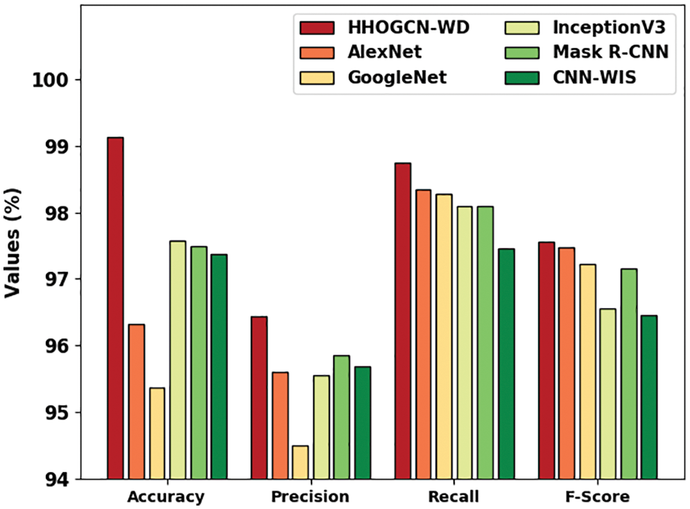
Figure 10: Comparative analysis of HHOGCN-WD approach with existing methodologies

Finally, for recal , the HHOGCN-WD method has rendered an increased recal of 98.74% whereas the AlexNet, GoogleNet, Inception v3, Mask RCNN, and CNN-WIS approach has reached reduced recal of 98.35%, 98.27%, 98.09%, 98.09%, and 97.46% correspondingly. At last, for Fscore , the HHOGCN-WD method has presented an increased Fscore of 97.56% whereas the AlexNet, GoogleNet, Inception v3, Mask RCNN, and CNN-WIS techniques have reached a reduced Fscore of 97.47%, 97.23%, 96.55%, 97.15%, and 96.46% correspondingly.

4  Conclusion

In this study, a new HHOGCN-WD technique has been developed for weed detection and classification for Precision Agriculture. The presented HHOGCN-WD technique mainly focuses on the identification and classification of weeds for precision agriculture. For image pre-processing, the HHOGCN-WD model utilizes BNF for noise removal. In addition, the CCNet model is utilized to derive a set of feature vectors. To detect and classify weed, the GCN model is utilized with the HHO algorithm as a hyperparameter optimizer to improve the detection performance. The experimental results of the HHOGCN-WD technique are investigated under the benchmark dataset. The results indicate the promising performance of the presented HHOGCN-WD model over other recent approaches.

Funding Statement: This research was partly supported by the Technology Development Program of MSS [No. S3033853] and by Basic Science Research Program through the National Research Foundation of Korea (NRF) funded by the Ministry of Education (No. 2020R1I1A3069700).

Conflicts of Interest: The authors declare that they have no conflicts of interest to report regarding the present study.

References

    1. W. H. Maes and K. Steppe, “Perspectives for remote sensing with unmanned aerial vehicles in precision agriculture,” Trends in Plant Science, vol. 24, no. 2, pp. 152–164, 2019. [Google Scholar]

    2. M. F. Aslan, A. Durdu, K. Sabanci, E. Ropelewska and S. S. Gültekin, “A comprehensive survey of the recent studies with uav for precision agriculture in open fields and greenhouses,” Applied Sciences, vol. 12, no. 3, pp. 1047, 2022. [Google Scholar]

    3. J. Champ, A. M. Fallas, H. Goëau, E. M. Montero, P. Bonnet et al., “Instance segmentation for the fine detection of crop and weed plants by precision agricultural robots,” Applications in Plant Sciences, vol. 8, no. 7, pp. e11373, 2020. [Google Scholar]

    4. S. Goel, K. Guleria and S. N. Panda, “Machine learning techniques for precision agriculture using wireless sensor networks,” ECS Transactions, vol. 107, no. 1, pp. 9229, 2022. [Google Scholar]

    5. E. Mavridou, E. Vrochidou, G. A. Papakostas, T. Pachidis and V. G. Kaburlasos, “Machine vision systems in precision agriculture for crop farming,” Journal of Imaging, vol. 5, no. 12, pp. 89, 2019. [Google Scholar]

    6. A. Chawade, J. van Ham, H. Blomquist, O. Bagge, E. Alexandersson et al., “High-throughput field-phenotyping tools for plant breeding and precision agriculture,” Agronomy, vol. 9, no. 5, pp. 258, 2019. [Google Scholar]

    7. D. Andujar and J. tinez-Guanter, “An overview of precision weed mapping and management based on remote sensing,” Remote Sensing, vol. 14, no. 15, pp. 3621, 2022. [Google Scholar]

    8. N. Delavarpour, C. Koparan, J. Nowatzki, S. Bajwa and X. Sun, “A technical study on UAV characteristics for precision agriculture applications and associated practical challenges,” Remote Sensing, vol. 13, no. 6, pp. 1204, 2021. [Google Scholar]

    9. A. E. Abouelregal and M. Marin, “The size-dependent thermoelastic vibrations of nanobeams subjected to harmonic excitation and rectified sine wave heating,” Mathematics, vol. 8, no. 7, pp. 1128, 2020. [Google Scholar]

  10. L. Zhang, M. M. Bhatti, E. E. Michaelides, M. Marin and R. Ellahi, “Hybrid nanofluid flow towards an elastic surface with tantalum and nickel nanoparticles, under the influence of an induced magnetic field,” The European Physical Journal Special Topics, vol. 231, no. 3, pp. 521–533, 2021. [Google Scholar]

  11. U. F. Ukaegbu, L. K. Tartibu, M. O. Okwu and I. O. Olayode, “Development of a light-weight unmanned aerial vehicle for precision agriculture,” Sensors, vol. 21, no. 13, pp. 4417, 2021. [Google Scholar]

  12. S. Khan, M. Tufail, M. T. Khan, Z. A. Khan and S. Anwar, “Deep learning-based identification system of weeds and crops in strawberry and pea fields for a precision agriculture sprayer,” Precision Agriculture, vol. 22, no. 6, pp. 1711–1727, 2021. [Google Scholar]

  13. M. H. Asad and A. Bais, “Weed detection in canola fields using maximum likelihood classification and deep convolutional neural network,” Information Processing in Agriculture, vol. 7, no. 4, pp. 535–545, 2020. [Google Scholar]

  14. K. Osorio, A. Puerto, C. Pedraza, D. Jamaica and L. Rodríguez, “A deep learning approach for weed detection in lettuce crops using multispectral images,” AgriEngineering, vol. 2, no. 3, pp. 471–488, 2020. [Google Scholar]

  15. O. Barrero and S. A. Perdomo, “RGB and multispectral UAV image fusion for gramineae weed detection in rice fields,” Precision Agriculture, vol. 19, no. 5, pp. 809–822, 2018. [Google Scholar]

  16. H. D. Han and J. K. Han, “Modified bilateral filter for feature enhancement in mesh denoising,” IEEE Access, vol. 10, pp. 56845–56862, 2022. [Google Scholar]

  17. L. Wang and X. Wang, “Dual-coupled cnn-gcn-based classification for hyperspectral and lidar data,” Sensors, vol. 22, no. 15, pp. 5735, 2022. [Google Scholar]

  18. L. Zhao, Y. Song, C. Zhang, Y. Liu, P. Wang et al., “T-Gcn: A temporal graph convolutional network for traffic prediction,” IEEE Transactions on Intelligent Transportation Systems, vol. 21, no. 9, pp. 3848–3858, 2019. [Google Scholar]

  19. Y. Zhang, R. Liu, X. Wang, H. Chen and C. Li, “Boosted binary harris hawks optimizer and feature selection,” Engineering with Computers, vol. 37, no. 4, pp. 3741–3770, 2021. [Google Scholar]

  20. K. Sudars, J. Jasko, I. Namatevs, L. Ozola and N. Badaukis, “Dataset of annotated food crops and weed images for robotic computer vision control,” Data in Brief, vol. 31, pp. 105833, 2020. [Google Scholar]

  21. Z. Wu, Y. Chen, B. Zhao, X. Kang and Y. Ding, “Review of weed detection methods based on computer vision,” Sensors, vol. 21, no. 11, pp. 3647, 2021. [Google Scholar]

  22. A. Subeesh, S. Bhole, K. Singh, N. S. Chandel, Y. A. Rajwade et al., “Deep convolutional neural network models for weed detection in polyhouse grown bell peppers,” Artificial Intelligence in Agriculture, vol. 6, pp. 47–54, 2022. [Google Scholar]