On Layout Optimization of Wireless Sensor Network Using Meta-Heuristic Approach

1  Introduction

A wireless sensor network (WSN) comprises of a large number of small, autonomous and spatially distributed sensor nodes [1]. These nodes can sense, process, and communicate relevant data with one another. Each sensor node contains a sensing transducer, a small memory, a radio transceiver, an embedded processor, and a battery for the power supply. The sensing transducer of a node is used for the collection of data from different environmental conditions such as sound, temperature, pressure, and motion. The sensing area of a node is determined by its sensing radius (RSense) [2], which is the maximum sensitivity range of its sensing transducer. Radio transceivers are used for the establishment of communication links among different sensor nodes. These links depend on the communication range (RComm) of transceivers, which is a maximum distance at which two nodes can communicate with each other. Sensor nodes cannot store the entire monitored data in their small memories. So, they send it to a central monitoring station called data sink at regular intervals, as shown in Fig. 1.

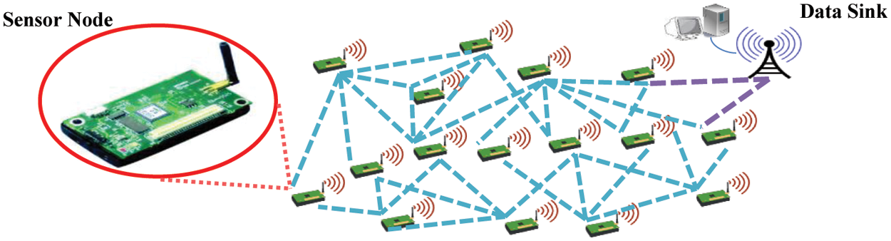
Figure 1: Illustration of a sensor node and a wireless sensor network

The embedded processors of sensor nodes transform the collected data into electrical signals and radio transceivers transmit these electrical signals to the data sink. Some sensor nodes may be unable to connect directly with a data sink because of limitations in their communication ranges and power sources. So, they use special intermediate nodes, the high energy communication nodes (HECN) as the gateways and send all of the monitored data to them. HECNs are directly connected with data sinks and provide external access to the network. The WSNs administrators collects the monitored data and send commands to the network through the HECN. In a WSN, every sensor node must connect to the HECN but all sensor nodes cannot establish direct communication links with HECN due to the communication range of nodes being small in comparison to the WSN size. Therefore, all those nodes, which are unable to directly communicate with HECN, establish multi-hop communication paths with HECN using intermediate nodes called relays. In this way, all nodes in a WSN can send data to the HECN by, at least, one of the two ways; directly, by using the direct communication path, or indirectly, by using the multi-hop communication paths [3]. Wireless sensor networks have been used in many applications. Examples are military activities of inspection and surveillance, environmental monitoring such as weather forecasting, biomedical purposes such as health conditions monitoring, and many more [1]. The diversity among these applications requires different deployment schemes of WSNs with varying parameters and constraints.

2  Literature Review

In the last two decades, several meta-hubristic techniques have been used to solve the WSN layout optimization problem, such as genetic algorithms (GA), particle swarm optimization (PSO), ant colony optimization (ACO), fish swarm optimization (FSO) and artificial bee colony algorithm (ABC). These meta-heuristic algorithms provide fast results to problems, but do not guarantee the provision of fully optimized and accurate solutions.

2.1 Multi Objective (MO) Optimization

Real world applications mostly depend on more than one objective functions. The solutions to such problems need simultaneous optimizations of these objective functions. This process is called multi-objective (MO) optimization, and it involves the optimization of a vector of solutions with more than one competing objectives. MO problems can be mapped in a vector form as a family of points known as a Pareto optimal set, where objectives are often conflicting. The optimal solution of one objective will not necessarily be the best solution for other objectives. Therefore, different solutions will produce trade-offs between different objectives and a non-dominated set of solutions is produced to represent the optimal solutions of all objectives. They provide output in the form of vectors, which contain Pareto in front of non-dominated solutions.

2.1.1 Multi Objective Genetic Algorithms

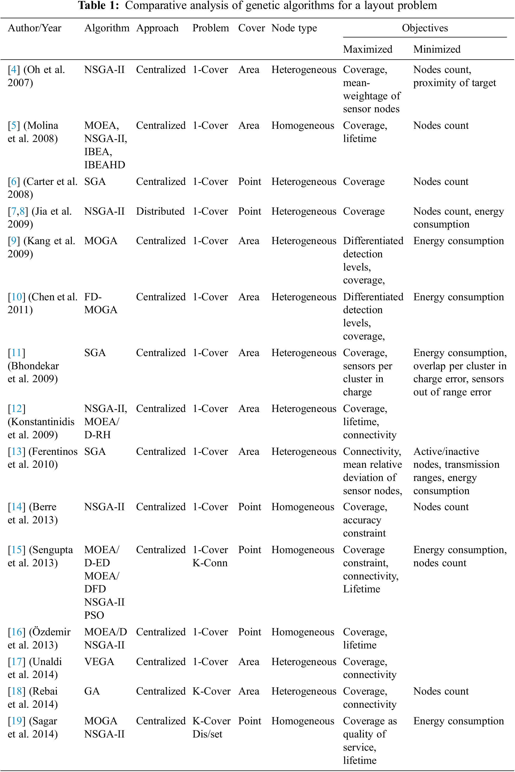
The genetic algorithms which can find non-dominating points from the population of solutions in parallel are categorized as multi-objective genetic algorithms (MOGA). Various MOGAs have been designed in the past and the literature review of these meta-heuristic techniques is presented in Table 1.

2.1.2 Multi Objective Particle Swarm Optimization

The literature review of PSO is presented in Table 2, along with its multi-objective variants.

3  Proposed Solution

In this research, a multi-objective firefly algorithm (MOFA) is proposed and applied for the layout optimization of WSNs.

3.1 Firefly Algorithm (FA)

The firefly algorithm (FA) approach is inspired by the natural light flashing behavior of fireflies, which they use to attract prey or their mating partners in the swarm. In this algorithm, the authors assume that all fireflies are unisexual [33]. The two fundamental properties of brightness (flashing light intensity) and attraction among fireflies are used in this algorithm under the following principles.

3.1.1 Brightness or Luminance Intensity

The luminance intensity or brightness of a firefly is controlled by the values of an objective function f(x). The luminance intensity (I) of a firefly at a particular location x in the solution space can be represented as I(x), which is directly proportional to the value of objective function f(x). The light in nature follows the inverse square law; when the distance from the light emitting source increases, the intensity decreases due to absorption in the environment. This principle is used in the algorithm to update the luminance intensity of fireflies.

The luminance intensity I(r) of a firefly at a distance r can be expressed as in (1), where I0 is the original light intensity of the firefly at a distance (r = 0), and γ is the fixed light absorption coefficient.

I(r) = I0e−γ r2 (1)

3.1.2 Attraction

In nature, attractiveness among the fireflies depends on the intensity of light they emit, and it is directly proportional to the brightness of fireflies. Therefore, for any two flashing fireflies, the less bright always has a tendency to move towards the brighter one. According to the principle of inverse square law, the values of attractiveness decrease among fireflies as the distance among them increases. The attractiveness β varies with the distance r between any two fireflies. As the attractiveness is proportional to the light intensity, so the attractiveness β is calculated according to (2), where β0 is the attractiveness at a distance (r = 0) from a firefly.

β(r) = β0e−γ rm,   with m≥1 (2)

3.1.3 Firefly Position Update

In the FA approach, as shown in Fig. 2, when a firefly i is attracted towards a firefly j, then the firefly i moves to the firefly j, and the new position x(i + 1) of firefly i can be calculated by using (3), Where xi and xj are the previous positions of firefly i and firefly j in solution space. The second term with β0 in (2) is introduced for the attraction, and the third term is for randomization with α as the controlling parameter, where rand is a random number between (0, 1). In exceptional cases, when all fireflies have the same brightness values, they are forced to move randomly in search space. The parameter γ controls the speed of convergence of the algorithm by changing the attractiveness.

x(i+1)= xi+ β0e−γ rij(xj − xi)+ α(rand −1/2) (3)

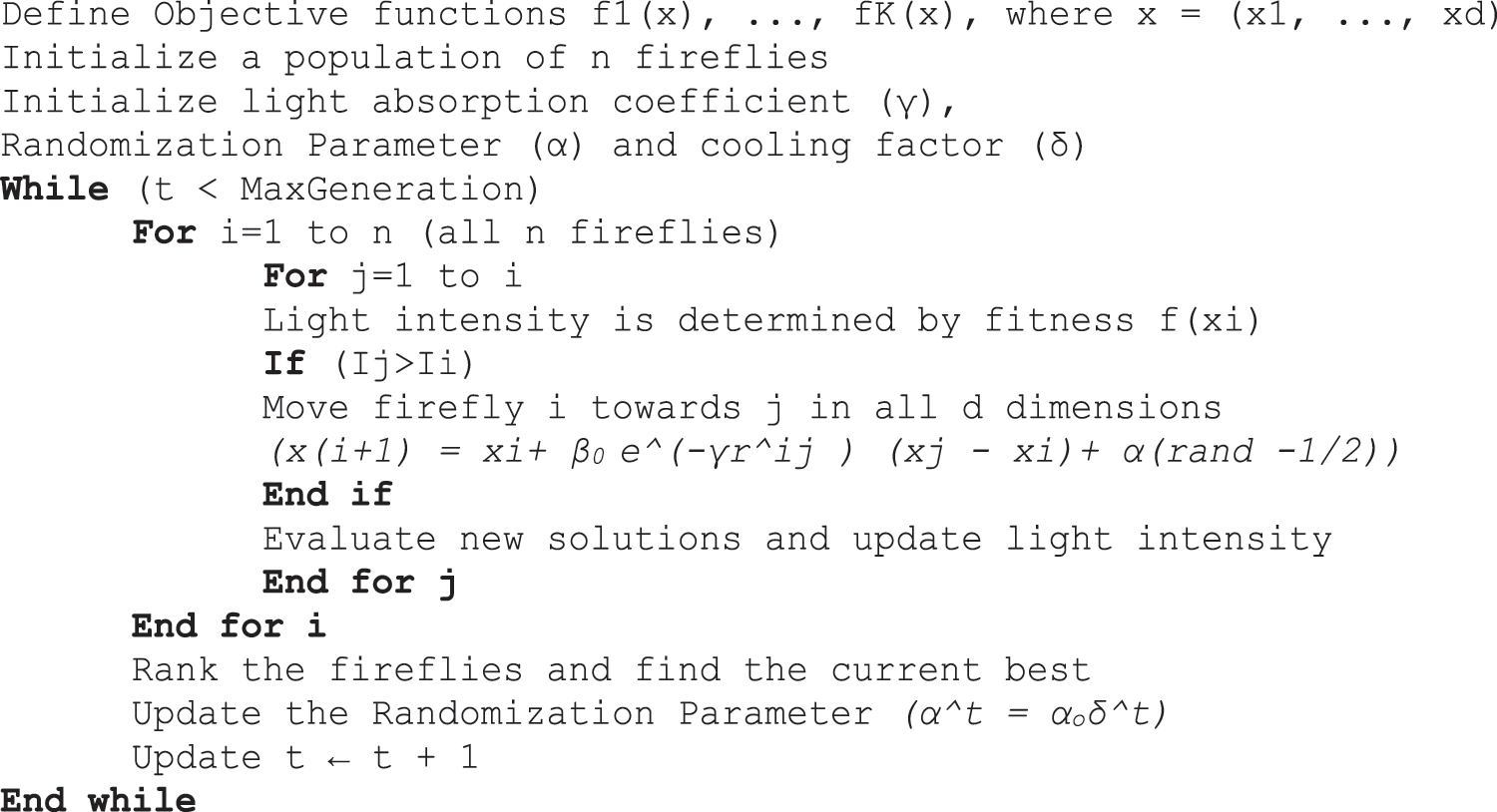
Figure 2: Pseudocode of the firefly algorithm

In [34], a new term, cooling factor delta (0 < δ < 1), has been introduced in the firefly algorithm to control the randomization parameter alpha (α) shown in (4). The randomization is reduced by multiplying it with delta after several iterations (t) of the algorithm so that the random walk become less aggressive towards the end of the algorithm. Here αo is the initial value of the random factor, and αt is the value of alpha for iteration number (t).

αt = αoδt (4)

3.2 Multi Objective Firefly Algorithm

A multi-objective firefly algorithm (MOFA) [35] is an extension of the FA. The MOFA finds a Pareto optimal front of non-dominated solutions for optimization of more than one competing objectives. In this algorithm, a random weight vector is used to store the best non-dominating solutions. In each iteration, these non-dominating solutions are found according to the fitness values of the objective functions and are passed to the next iteration for the calculation of more non-dominating solutions. The output is a vector containing the final non-dominated solutions.

4  Methodology

The optimal layout designing problem is related to the selection of physical positions of sensor nodes in a way that they entirely cover a geographical area or a set of targets [2,36]. The main goal of layout optimization is to show that “how well a geographical region or a set of targets are monitored by deployed sensor nodes in a WSN”. The ideal solution of this problem belongs to the NP-hard combinatorial class and requires the optimizations of a large number of competing objectives like coverage, connectivity, lifetime, cost, energy efficiency, scalability, and fault tolerance of WSNs. The layout optimization problem becomes more complex when the size of WSNs and diversity among sensor nodes increases. For optimal layout designing, it becomes challenging to calculate the objectives of large-scale WSNs in a simple way, because of the limitations in energy, detection, communication, and computational resources of sensor nodes.

The layouts directly affect the efficiency and monitoring capability of WSNs, and if layout optimization is not considered while deploying the sensor nodes, then WSNs behavior may become unpredictable with high network failure rates, bad area coverage, and frequent disconnections. This degradation in WSNs drastically influences the functionality and performance of real-time applications.

4.1 WSNs Solution Representation

In this solution, a two-dimensional plane is used for the representation of monitoring area to be covered by the deployed sensor nodes. A distance vector (DV) is used to represent a single solution of each problem, and the size of this vector depends on the total number of sensor nodes as in (5). Each sensor node in the network has an active or inactive state and is located at a specific position in the monitoring region. Position of each node in the solution is represented by (x, y) coordinates in the two-dimensional plane, and n is the total number of nodes.

DV [n]=[(x1,  y1),  (x2,  y2),  (x2,  y2) … (xn, yn)] (5)

When the position coordinates of the monitoring area (length × width) are taken as 100 × 100, then for all single and multi-objective problems, two vectors X = {0, 1, 2……100} and Y = {0, 1, 2……100} are used to represent (x, y) coordinates of the two-dimensional area points. A third vector contains the information of active and inactive sensor nodes in the case of homogeneous WSNs and the size of this vector is set to “n”. This vector is used for the calculation of the maximum and the minimum number of sensor nodes for all problems. For heterogeneous WSNs, this third vector is used to represent the various sensing ranges of nodes (RSense). In all of our experiments, complete solutions of optimization problems are encoded in the form of firefly chromosomes.

4.1.1 Chromosome, Firefly and Particle Encoding for Homogeneous WSNs

In homogeneous WSNs, all of the nodes are considered identical with the same sensing range (RSense) and no encoding is required for representing the node properties. Each firefly is encoded as a complete layout solution of a WSN. The sensor nodes are encoded as genes of a chromosome, and information about their positions and active and inactive modes is included. In the encoding of each chromosome, an active-inactive (A/I) mode bit is used, which is set when a node is considered active and could take part in the fitness calculation of the designed solution, as shown in Fig. 3. Position of each node in the chromosome is dependent on the coordinates of the deployment plane. For two-dimensional planes, the position of each node i along (x, y) coordinates are encoded with an equal number of bits for both axes.

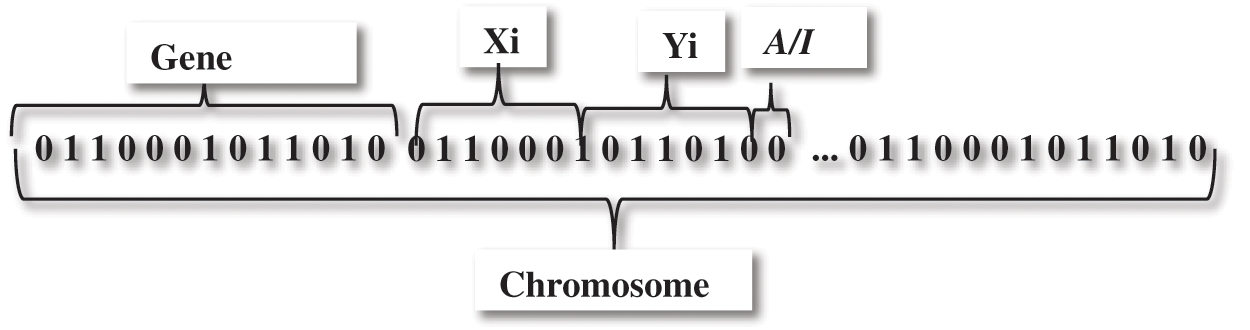
Figure 3: Chromosome with binary encoding for a homogeneous WSN

4.2 Fitness Calculation

The fitness calculation of each solution is performed by taking the weighted sum of all objective functions. The fitness calculation methods for coverage, number of nodes, connectivity, lifetime, and energy consumption of WSNs are presented here.

4.2.1 Number of Nodes

The number of nodes for each solution is calculated using the number of active-inactive (A/I) mode bits. In solutions of homogeneous WSNs, a single active-inactive (A/I) mode bit is used to calculate active nodes while set to one.

4.2.2 Coverage

There are two methods available for the calculation of coverage; one is grid-based, and the second is area-based. In both of the techniques, a binary sensing model is used where the sensing area of a node is considered as a circular disk with a fixed sensing range (RSense). An object present at a distance less than the sensory range can be sensed by a node. Here the detection probability Pi of a sensor node Si is calculated using the Euclidean distance from the center of the node to the target point Ti with respect to the fixed sensing radius RSense according to (6)

Pi={1 if dist(Si,Ti)<RSense0 Otherwise (6)

In the area-based method, the sensor nodes are randomly distributed in the monitoring area. The area covered by an individual sensor node is measured depending on its sensing radius (RSense), which is the same for all sensor nodes in a homogeneous WSN. The total area covered by these nodes is calculated, and the overlap among sensor nodes is subtracted to get full area coverage according to (7).

Area Coverage=∑iN⁡πRsense 2−overlap(Sensor1… SensorN) (7)

In the grid-based method, the whole monitoring region is divided in square grids of equal sizes. Euclidean distance of sensor nodes from the center point of each grid is calculated to determine if a grid is completely covered by some of the nodes or not. The maximum area covered by any sensor node i at position (xi, yi) is calculated by using the sensing radius (RSense). The total covered grid points of the grid are then normalized by the total points in the area according to (8).

Point Coverage=[Ui=1n Rsense2(xi,  yi)]/Total Points (8)

The grid-based method is fast when the number of sensor nodes and the monitoring area or points are small, but it becomes slow when the WSNs size grows due to the presence of a large number of nodes. To avoid the performance degradation of the algorithm, the area-based coverage calculation method is used for area coverage and the grid-based method is used for point coverage.

4.2.3 Connectivity

A WSN is considered connected when there exists at least one single or multi-hop communication path between all of the sensor nodes and the data sink. The main goal of the optimization algorithms is to minimize the number of disconnected nodes in the network, so that a fully connected network is attained. The connectivity of each layout solution is tested by creating a graph with nodes as its vertices, and a minimal spanning tree is developed with the data sink as the root node. Two nodes i and j are considered connected if the distance (dij) between them is less than their communication radius (RComm) and the edge weight (EWij) is set to the distance (dij) between them as in (9). Then the Bellman Ford algorithm of single source shortest path is applied to calculate the shortest paths from the data sink, which is placed at the middle of the monitoring area, to all of the active nodes. The nodes are considered disconnected when there exists no feasible path to the data sink.

EWij={dij if dij<RCOMM∞  otherwise (9)

4.2.4 Energy Consumption

Every node in a WSN may perform several different tasks such as maintenance, sensing, processing, transmission and reception of data to and from other sensor nodes. These operations consume energy and for an optimal layout, the minimum data transmission path must be used to conserve this energy. For the calculation of energy consumption (ECi) at each node i, the data transmission cost for the shortest path (Pathi) to the data sink is calculated using the minimal spanning tree method. The neighboring nodes (Ini) from which data can be received are calculated and the node maintenance energy (Mi), the transmission energy (Trai), and the reception energy (Reci) are summed up according to (10). The energy consumption of the whole network is the sum of the energies consumed by the active nodes (n) in the network and is calculated using (11).

ECi=Mi+Pathi×Trai+Ini ×Reci (10)

Total Energy=∑i=1n⁡ECi (11)

4.2.5 Life Time

The life time of a WSN depends on the failure of the first node in the network. The life time of a single node (LTi) is calculated using the initial energy (IEi) and the consumed energy estimate (ECi) of each node. The time until which a node can work is calculated as in (12). The network breaks down when the first node fails and the life time of the whole network is calculated as the minimum lifetime of an active node i according to (13).

LTi=IEi/ECi (12)

Life Time=Min{LTi} (13)

4.3 Experimental Setup

The performance of MOFA is tested by comparing it with the multi-objective genetic algorithms (IBEA, NSGA-II) and the particle swarm optimizers (SMPSO, OMOPSO) according to the parameter settings presented in Table 3. In all of our experiments, the randomization parameter (α) for MOFA is initialized with low values. The random movement of fireflies toward the end of the algorithm run is increased by using the cooling factor delta (δ). In the parameter settings of MOFA, the randomization is increased by 15% after every 20 iterations of the algorithm.

5  Results and Discussion

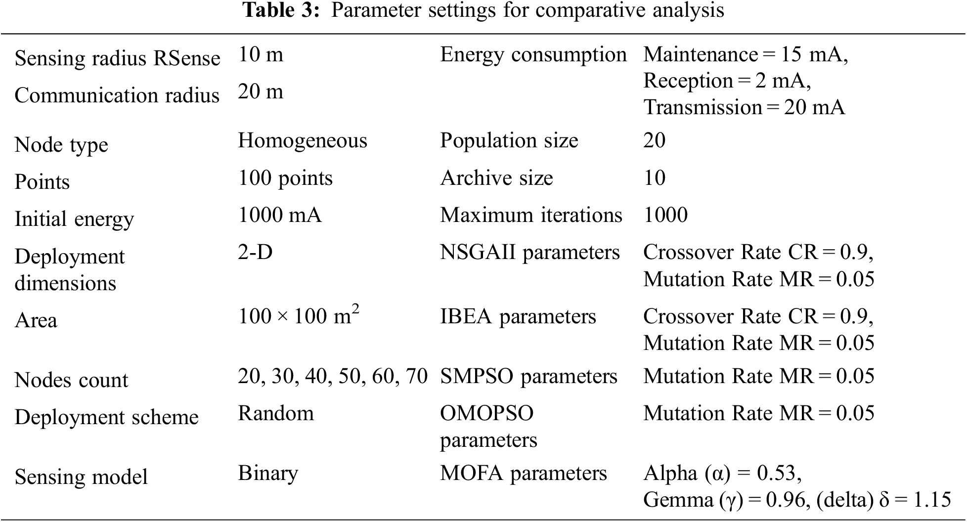
The results for best non-dominated solutions are obtained by varying the number of homogeneous sensor nodes in the range (20–70) with a swarm size of 20. For all the experiments, 1000 iterations are run to find the Pareto optimal solutions.

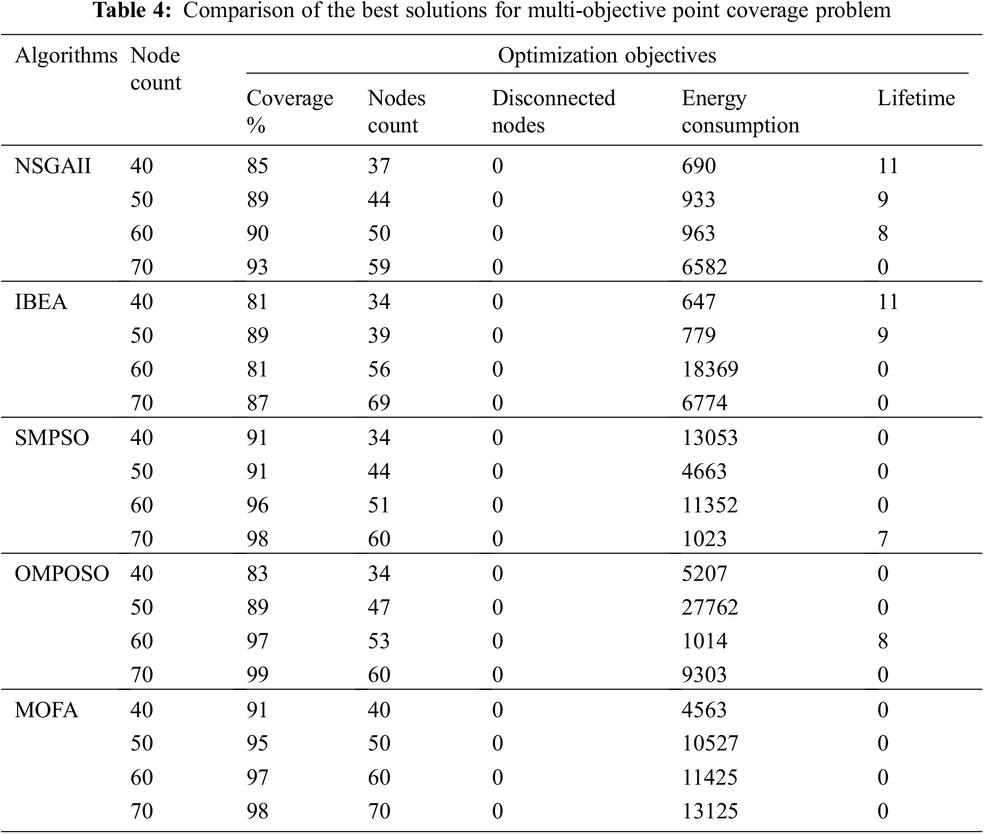
5.1 Multi Objective Point Coverage Problem (MO Point Cover)

A solution with five competing objective is designed for the multi-objective point coverage problem. It involves the maximization of point coverage, lifetime and connectivity of sensor nodes, along with the minimization of energy consumption and the number of sensor nodes. The results are presented in Table 4.

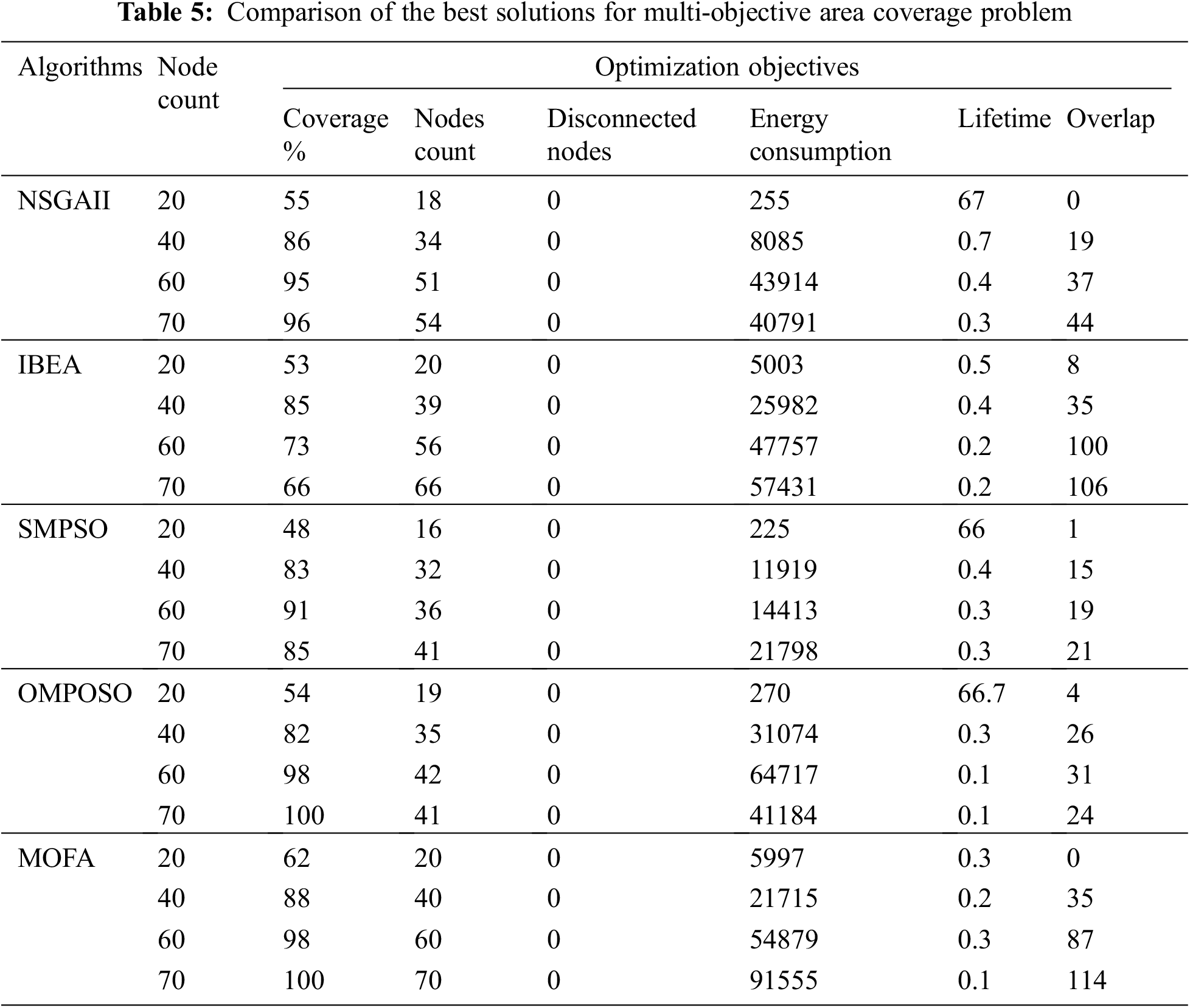
5.2 Multi Objective Area Coverage Problem (MO Area Cover)

The solution for the multi-objective area coverage problem is formed with the simultaneous optimization of six objectives. These objectives are the maximization of area coverage, lifetime and connectivity of sensor nodes and the minimization of energy consumption, overlapped region and the number of deployed sensor nodes for homogeneous WSNs. The results of this experiment are presented in Table 5.

5.2.1 Comparison of Area Coverage Solutions

WSNs layouts obtained by plotting the best solutions of multi-objective area coverage problem are shown in the Fig. 4. These layouts are designed by MOFA, NSGAII, IBEA, SMPSO and OMOPSO with a varying number of nodes. It can be observed from the results that NSGAII and IBEA provide layouts with low area coverage and these algorithms did not explore the solution space completely. The layouts generated by IBEA and NSGAII left empty outer regions of the monitoring area. The layout schemes generated by MOFA, SMPSO and OMOPSO are better in the distribution of nodes. MOFA designed better layout schemes with evenly distributed nodes in the whole monitoring area and provided 100% area coverage with a fully connected network. OMOPSO generated the second best layouts and it also attained 100% area coverage of connected WSNs.

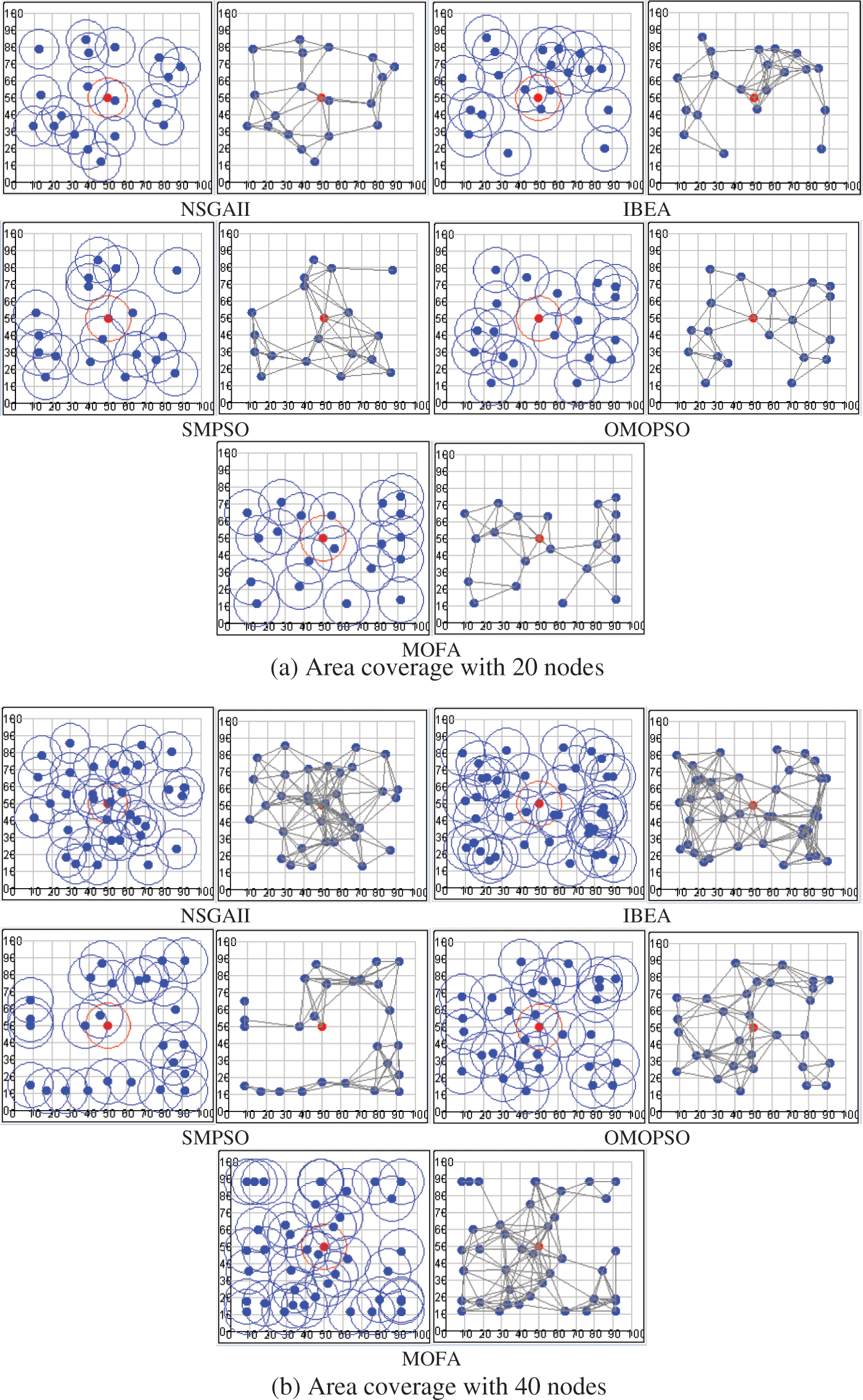
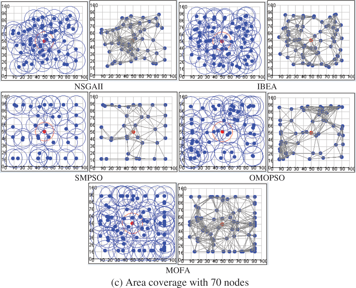
Figure 4: Layouts of homogeneous WSNs for the multi-objective area coverage problem

5.3 Discussion

The results show that MOFA and OMOPSO found near optimal solutions and provided the best solutions with 100% point and area coverage with full connectivity of the network. SMPSO and NSGAII found better results than IBEA with 100% connectivity. The closeness of the non-dominated solutions generated by the multi-objective algorithms to the true Pareto Front can be determined if the true Pareto Front is known. In the absence of the information about the true front, the values of spread is a quality indicator of solutions. For the performance comparison of multi-objective algorithms, we use the hyper volume quality indicator, and its value is maximized to gain good quality non-dominated solutions. The algorithm with a high hyper volume value of non-dominated solutions is considered superior to those with low hyper volume values. The comparison of the hyper volume and spread indicators for non-dominated solutions generated by multi-objective algorithms MOFA, NSGA-II, IBEA, SMPSO and OMOPSO are shown in Figs. 5 and 6.

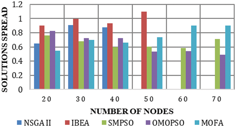
Figure 5: Non-dominated solutions spread for the homogeneous point coverage problem

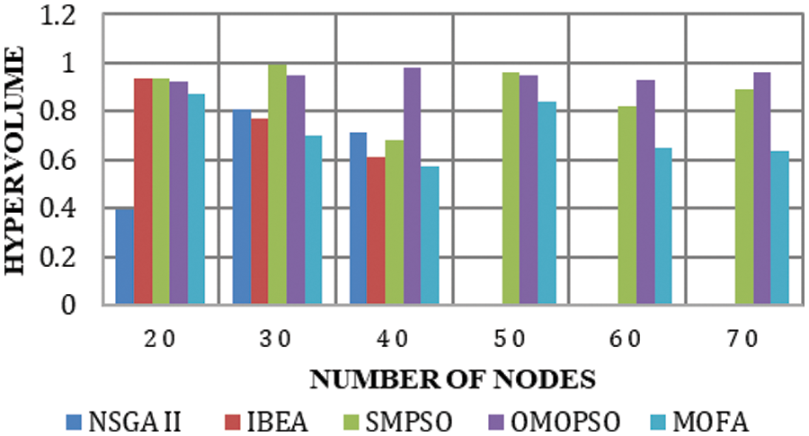
Figure 6: Non-dominated solutions hyper volume for the homogeneous area coverage problem

The spread values of solutions generated by MOFA are low when the number of nodes is small, but they improve with increments in nodes. The solution spread values of MOFA are better than SMPSO and OMOPSO with 50, 60 and 70 nodes. NSGA-II and IBEA show high spread values with a small number of nodes but provide a zero spread of solutions with 60 and 70 nodes, as shown in Fig. 5.

The hyper volumes of solutions generated by MOFA are lower than values provided by OMOPSO and SMPSO but higher than NSGA-II and IBEA values. This shows that solutions generated by MOFA are dominated by SMPSO and OMOPSO but better than solutions of NSGA-II and IBEA, as shown in Fig. 6. The NSGA-II and IBEA hyper volume values are zero with 50, 60 and 70 nodes.

6  Conclusion

Our experiments show that the multi-objective firefly algorithm efficiently optimizes the layout schemes for homogeneous WSNs by providing Pareto optimal front of non-dominated solutions. The algorithm well utilizes the exploration and exploitation capabilities associated with meta-heuristic algorithms. Our results show that MOFA maximizes the area coverage to 100% and the point coverage to 99%. It is also noticeable that the layout diagrams obtained from our simulations show improvement in energy consumption and lifetime of the network, which leads to ideal layouts of WSNs. Moreover, MOFA is scalable for large-scale wireless sensor networks. Comparative analysis with SMPSO, OMOPSO, NSGAII and IBEA show that MOFA provides near optimal results with a better convergence speed.

This study can be further extended for the optimization of heterogeneous WSNs with probabilistic sensing models. MOFA can also be applied to other multi-objective optimization problems, such as localization, energy-aware routing, clustering and scheduling of WSNs.

Acknowledgement: The authors extend their appreciation to the Deanship of Scientific Research at Imam Mohammad Ibn Saud Islamic University for funding this work through Research Group No. RG-21-07-09.

Funding Statement: This research has been funded by the Deanship of Scientific Research at Imam Mohammad Ibn Saud Islamic University through Research Group No. RG-21-07-09.

Conflicts of Interest: The authors declare that they have no conflicts of interest to report regarding the present study.

References

1. I. F. Akyildiz, T. Melodia and K. R. Chowdhury, “A survey on wireless sensor networks,” Computer Networks, vol. 51, no. 4, pp. 921–960, 2007. [Google Scholar]
2. C. F. Huang and Y. C. Tseng, “The coverage problem in a wireless sensor network,” ACM Transactions on Mobile Networks and Applications, vol. 10, no. 4, pp. 519–528, 2005. [Google Scholar]
3. A. Sangwan and R. P. Singh, “Survey on coverage problems in wireless sensor networks,” Journal Wireless Personal Communications, vol. 80, no. 4, pp. 1475–1500, 2015. [Google Scholar]
4. S. C. Oh, C. H. Tan, F. W. Kong, Y. S. Tan, K. H. Ng et al., “Multi-objective optimization of sensor network deployment by a genetic algorithm,” in Proc. IEEE Conf. on Evolutionary Computation, Singapore, pp. 3917–3921, 2007. [Google Scholar]
5. G. Molina, E. Alba and E. G. Talbi, “Optimal sensor network lay-out using multi-objective meta-heuristics,” Journal of Universal Computer Science, vol. 14, no. 15, pp. 2549–2565, 2008. [Google Scholar]
6. B. Carter and R. Ragade, “An extensible model for the deployment of non-isotropic sensors,” in IEEE Sensors Applications Symp., Atlanta, GA, USA, pp. 22–25, 2008. [Google Scholar]
7. J. Jia, J. Chen, G. Chang, Y. Wen and J. Song, “Multi-objective optimization for coverage control in wireless sensor network with adjustable sensing radius,” Computers and Mathematics with Applications, vol. 57, no. 11–12, pp. 1767–1775, 2009. [Google Scholar]
8. J. Jia, J. Chen, G. Chang and Z. Tan, “Energy efficient coverage control in wireless sensor networks based on multi-objective genetic algorithm,” Computers and Mathematics with Applications, vol. 57, no. 11–12, pp. 1756–1766, 2009. [Google Scholar]
9. C. W. Kang and J. H. Chen, “An evolutionary approach for multi-objective 3D differentiated sensor network deployment,” in Proc. IEEE Int. Conf. on Computational Science and Engineering, Vancouver, BC, Canada, vol. 1, pp. 187–193, 2009. [Google Scholar]
10. J. Chen and C. Kang, “A force-driven evolutionary approach for multi-objective 3D differentiated sensor network deployment,” International Journal of Ad Hoc and Ubiquitous Computing, vol. 8, pp. 85–95, 2011. [Google Scholar]
11. A. P. Bhondekar, R. Vig, M. L. Singla, C. Ghanshyam and P. Kapur, “Genetic algorithm based node placement methodology for wireless sensor networks,” in Proc. Int. Multi-Conf. of Engineers and Computer Scientists, Hong Kong, vol. 1, pp. 18–20, 2009. [Google Scholar]
12. A. Konstantinidis, K. Yang and Q. Zhang, “Problem-specific encoding and genetic operation for a multi-objective deployment and power assignment problem in wireless sensor networks,” in Proc. IEEE Int. Conf. on Communications, Dresden, Germany, pp. 1–6, 2009. [Google Scholar]
13. K. P. Ferentinos and T. A. Tsiligiridis, “A memetic algorithm for optimal dynamic design of wireless sensor networks,” Computer Communications, vol. 33, no. 2, pp. 250–258, 2010. [Google Scholar]
14. M. L. Berre, F. Hnaien and H. Snoussi, “A multi-objective modeling of K-coverage problem under accuracy constraint,” in Proc. IEEE 5th Int. Conf. on Modeling, Simulation and Applied Optimization, Hammamet, Tunisia, pp. 1–6, 2013. [Google Scholar]
15. S. Sengupta, S. Das, M. D. Nasir and B. K. Panigrahi, “Multi-objective node deployment in WSNs: In search of an optimal trade-off among coverage, lifetime, energy consumption, and connectivity,” Engineering Applications of Artificial Intelligence, vol. 26, no. 1, pp. 405–416, 2013. [Google Scholar]
16. S. Özdemir, A. A. Bara’a and Ö. A. Khalil, “Multi-objective evolutionary algorithm based on decomposition for energy efficient coverage in wireless sensor networks,” Wireless Personal Communications, vol. 71, no. 1, pp. 195–215, 2013. [Google Scholar]
17. N. Unaldi and S. Temel, “Wireless sensor deployment method on 3D environments to maximize quality of coverage and quality of network connectivity,” in Proc. World Congress Engineering and Computer Science, San Francisco, USA, vol. 2, pp. 2078–0966, 2014. [Google Scholar]
18. M. Rebai, H. Snoussi, F. Hnaien and L. Khoukhi, “Sensor deployment optimization methods to achieve both coverage and connectivity in wireless sensor networks,” Computers & Operations Research, vol. 59, pp. 11–21, 2015. [Google Scholar]
19. A. K. Sagar and D. K. Lobiyal, “A multi-objective optimization approach for lifetime and coverage problem in wireless sensor network,” in Intelligent Computing, Networking, and Informatics, New Delhi: Springer, pp. 343–350, 2014. [Google Scholar]
20. X. Wang, S. Wang and J. J. Ma, “An improved co-evolutionary particle swarm optimization for wireless sensor networks with dynamic deployment,” Sensors, vol. 7, no. 3, pp. 354–370, 2007. [Google Scholar]
21. J. Hu, J. Song, M. Zhang and X. Kang, “Topology optimization for urban traffic sensor network,” Tsinghua Science & Technology, vol. 13, no. 2, pp. 229–236, 2008. [Google Scholar]
22. N. A. B. A. Aziz, A. W. Mohemmed and M. Y. Alias, “A wireless sensor network coverage optimization algorithm based on particle swarm optimization and voronoi diagram,” in IEEE Int. Conf. on Intelligent and Advanced Systems, Okayama, Japan, pp. 602–607, 2009. [Google Scholar]
23. P. M. Pradhan, V. Baghel, G. Panda and M. Bernard, “Energy efficient layout for a wireless sensor network using multi-objective particle swarm optimization,” in IEEE Int. Advance Computing Conf., Patiala, India, pp. 65–70, 2009. [Google Scholar]
24. S. M. A. Salehizadeh, A. Dirafzoon, M. B. Menhaj and A. Afshar, “Coverage in wireless sensor networks based on individual particle optimization,” in IEEE Int. Conf. on Networking, Sensing and Control, Chicago, IL, USA, pp. 501–506, 2010. [Google Scholar]
25. W. W. Ismail and S. A. Manaf, “Study on coverage in wireless sensor network using grid based strategy and particle swarm optimization,” in IEEE Asia Pacific Conf. on Circuits and Systems, Kuala Lumpur, Malaysia, pp. 1175–1178, 2010. [Google Scholar]
26. N. A. B. A. Aziz, A. W. Mohemmed, M. Y. Alias, K. A. Aziz and S. Syahali, “Coverage maximization and energy conservation for mobile wireless sensor networks: A two phase particle swarm optimization algorithm,” in IEEE 6th Int. Conf. on Bio-Inspired Computing: Theories and Applications, Penang, Malaysia, pp. 64–69, 2011. [Google Scholar]
27. D. K. Chaudhary and R. L. Dua, “Application of multi objective particle swarm optimization to maximize coverage and lifetime of wireless sensor network,” International Journal of Computational Engineering Research, vol. 2, no. 5, pp. 1628–1633, 2012. [Google Scholar]
28. G. Y. Tang, M. Z. Zhou and D. Yang, “Adaptive design of wireless sensor networks based on hybrid immune particle swarm optimization,” in Proc. IEEE 3rd Int. Conf. on System Science, Engineering Design and Manufacturing Informatization, Chengdu, China, vol. 2, pp. 292–295, 2012. [Google Scholar]
29. V. Loscrí, E. Natalizio, F. Guerriero and G. Aloi, “Particle swarm optimization schemes based on consensus for wireless sensor networks,” in Proc. of the 7th ACM Workshop on Performance Monitoring and Measurement of Heterogeneous Wireless and Wired Networks, Cyprus, pp. 77–84, 2012. [Google Scholar]
30. Y. Hu, “Minimal K-covering set algorithm based on particle swarm optimizer,” Journal of Networks, vol. 8, no. 12, pp. 2872–2877, 2013. [Google Scholar]
31. I. Maleki, S. R. Khaze, M. M. Tabrizi and A. Bagherinia, “A new approach for area coverage problem in wireless sensor networks with hybrid particle swarm optimization and differential evolution algorithms,” International Journal of Mobile Network Communications, vol. 3, pp. 61–75, 2013. [Google Scholar]
32. M. Gu, Y. Yan, C. Su and Z. Zuo, “An efficient hybrid approach based on PSO, TS and SA for the efficient-energy coverage problem,” Journal of Computational Information Systems, vol. 9, no. 3, pp. 1121–1129, 2013. [Google Scholar]
33. X. S. Yang, “Firefly algorithms for multimodal optimization,” in Int. Symp. on Stochastic Algorithms, Berlin, Heidelberg, Springer, pp. 169–178, 2009. [Google Scholar]
34. X. S. Yang and H. X. Xingshi, “Firefly algorithm: Recent advances and applications,” International Journal of Swarm Intelligence, vol. 1, no. 1, pp. 36–50, 2013. [Google Scholar]
35. X. S. Yang, “Multiobjective firefly algorithm for continuous optimization,” Engineering with Computers, vol. 29, no. 2, pp. 175–184, 2013. [Google Scholar]
36. G. Xing, X. Wang, Y. Zhang, C. Lu, R. Pless et al., “Integrated coverage and connectivity configuration for energy conservation in sensor networks,” ACM Transactions on Sensor Networks, vol. 1, no. 1, pp. 36–72, 2005. [Google Scholar]
Cite This Article
Copyright © 2023 The Author(s). Published by Tech Science Press.
This work is licensed under a Creative Commons Attribution 4.0 International License , which permits unrestricted use, distribution, and reproduction in any medium, provided the original work is properly cited.
Downloads
Citation Tools