AI Method for Improving Crop Yield Prediction Accuracy Using ANN

1  Introduction

Agriculture is the study and practice of farming, which includes soil cultivation for agricultural development and animal husbandry, among other things. Despite farmers’ agricultural skills, there is a significant gap between scientific and technological knowledge in rural areas. To combat a host of problems—from dwindling arable land and scarcity of water to significantly reducing organic material and multi-nutrient deficiencies, not to mention the people’s exodus from farming—Indian farmers have switched their attention from conventional farming to precision agriculture. CYP is one of precision agriculture’s most challenging problems, and many models have been proposed. This function involves the usage of numerous data sets because Crop Production (CP) is affected by many ambient components, specifically metrological factors, soil, climate, germination and fertilizer usage [1].

Precision agriculture requires a thorough understanding of the links between yield, climate, and soil qualities. Identifying tools for reliably quantifying the links between soil and weather conditions and crop output is a vital first step. The environment is the dominant factor affecting whether a crop is suitable for a particular place. The crop’s potential output is primarily influenced by the atmosphere. The setting involves more than 50% of crop varieties. In crops like cereals, legumes, and vegetables, the tested temperature during early seed development can lower seed size, quantity, and fertility, delay germination, and reduce seed vigour. Before planting, soil moisture can affect crop output by altering seedling emergence and roots, making it a crucial factor in agronomic management. However, the extent to which initial soil moisture affects crop output has not been defined, particularly in emerging regions where food security is a key issue, and there are field data on soil moisture and weather conditions. Germination and moisture content were shown to be correlated, but germination sharply declined when the moisture content dropped below 25% [2]. Agricultural experts are improving agricultural and rural statistics and developing methods for more accurate CYP based on agricultural data sets. The main objective of agricultural planning is to increase CP while conserving limited land resources.

The field of Artificial Intelligence (AI), also known as computational intelligence, seeks to create computer programmes that can learn complicated real-world problems just like people do. Complexity and uncertainty arise when challenging problems are solved using conventional programming techniques. The basic idea behind the creation of evolutionary algorithms is to mimic human intelligence in order to resolve reasoning problems. Artificial Neural Network (ANN) techniques can create an automated model that uses computer intelligence to challenge real-world problems [3]. After processing the input data, the algorithm generates an output known as a “model” that aids in forecasting the CY before the harvest. Implementing computing intelligence in real life has some drawbacks, such as the lack of data to train the model on, the presence of contaminants in the dataset, and the use of additional features that are low prediction model performance and increase computational costs. More attributes used to train the model will also result in overfitting, preventing the results of computational learning models from generalising. This research was cutting-edge because it meticulously collected meteorological data from the appropriate agencies. And the effects of weather-related conditions were accurately studied. The primary goal of this work is to improve the performance of ANNs by streamlining the input parameters fed to the input layers, decreasing computation time, enhancing result accuracy, and pinpointing the elements that influence crop output [4].

Machine Learning (ML) techniques are supported in increasing CY rate output. ML technologies are applied in various fields, from evaluating user behaviour in marketplaces to predicting customer smartphone usage. For specific years, ML has been used in agriculture. This shows that assessing agricultural production is a multi-stage process rather than a simple one. CYP methods can now fairly assess actual yields, but greater yield forecast performance is still necessary [5]. The CYP accuracy is obtained using a well-known algorithm called ML for numerous parameters. ML may acquire knowledge from data sets by identifying correlations between variables. The models must be trained with data sets that depict the outcomes based on previous experience [6].

The most extensively used ML method for CYP accuracy for the given crop is ANN [7]. The advantage of ANN is that it learns directly from examples without evaluating the parameters using statistical methods [8]. ANN has been used to predict CP in several crops, including wheat, kiwifruit, and rice.

However, less work has been carried out in Tamil Nadu to determine agricultural production concerning meteorological factors and soil nutrients, and this research is being carried out for a better understanding of CYP in Tamil Nadu for different CP [9]. The ANN model is developed as a structure of training procedures that forecasts CP based on meteorological conditions and soil nutrients, and three methodologies were tested and assessed. The literature construction of an ANN’s training process on different algorithms indicates that, as previously stated, ANNs are widely used in various non-linear practical problems [10]. Creating an ANN requires at least three layers: input, hidden, and output. The information is obtained using a NN to find relationships in data [11]. The raw data is received by the first layer, which is processed before being fed into the third hidden layer. The data is subsequently sent from the hidden third layer to the final output, which generates the production of a process. The objective of this work is to demonstrate the predictive abilities of Levenberg–Marquardt (LM), Bayesian Regularization (BR), and Scaled Conjugate Gradient (SCG) [12]. The capacity to predict reflective intelligence in the data was applied with three distinct backpropagation algorithms. The best model was scrutinised as LM by examining the high correlation rate and the low computational time with the fulfilled mean squared error value [13].

CYP is an essential agricultural problem [14]. All farmers always try to know how much yield they will get from their prospects. In the past, CYP was designed by analyzing a farmer’s previous experience with a particular crop. The CY primarily depends on weather conditions, soil nutrients, and temperature. Accurate data about the history of CY is vital for decision-making related to agricultural risk management [15].

This primary research focuses on

•   To forecast the CY for different crops by considering temperature, climatic effect, and soil features.

•   To use different ML algorithms for CYP.

•   This work compares the performance of ML algorithms to measure prediction accuracy.

•   To improve the accuracy of CYP.

The paper presents the empirical results and analysis of different ML algorithms. This article is structured as follows: Section 2 describes the ML algorithms used for CYP. Section 3 discusses the proposed methodology. Section 4 discusses the study area of the field that has been considered. Section 5 includes the result and discussions about the prediction accuracy of different ML algorithms, and The summary of this paper is found in Section 6.

2  Related Works

The most prominent and accurate numerical tool to explore the correlations between variables is ANN. An ANN is a computer-based structure comprising multiple simple processing units operating in parallel [16]. The building blocks of ANN are shown in Fig. 1. In order to examine the effect of predictors on target variable quantity, the third layer comprises activation functions and analyses the weights of the variables. The process can be completed in the output layer, and the findings are delivered with a modest assessment error [17]. The backpropagation method generates associations between inputs and outputs throughout the training process. The preceding is how the backpropagation training algorithm works. The weights are modified once the input values are propagated to a hidden layer, and the sensitivities are communicated back to lower the error. Predictive analytics assumes that things will stay mostly the same in the future. Neurons within the same layer of an ANN are not expected to communicate with one another. Instead, the input, hidden, and output layers are considered to be placed sequentially. A prediction convergence on an ANN’s size and structure is not guaranteed and is determined through trial and error. The drawback of ANNs is that they can only process numerical data. Before using ANN, problems are converted into numerical numbers. The display mechanism chosen here will directly impact the network’s performance. It is based on the user’s skill. It is important to remember that while ANN networks, an area of science in development, gain more benefits every day, their drawbacks are being eliminated. It indicates that ANNs will play a more significant and prominent role in our lives.

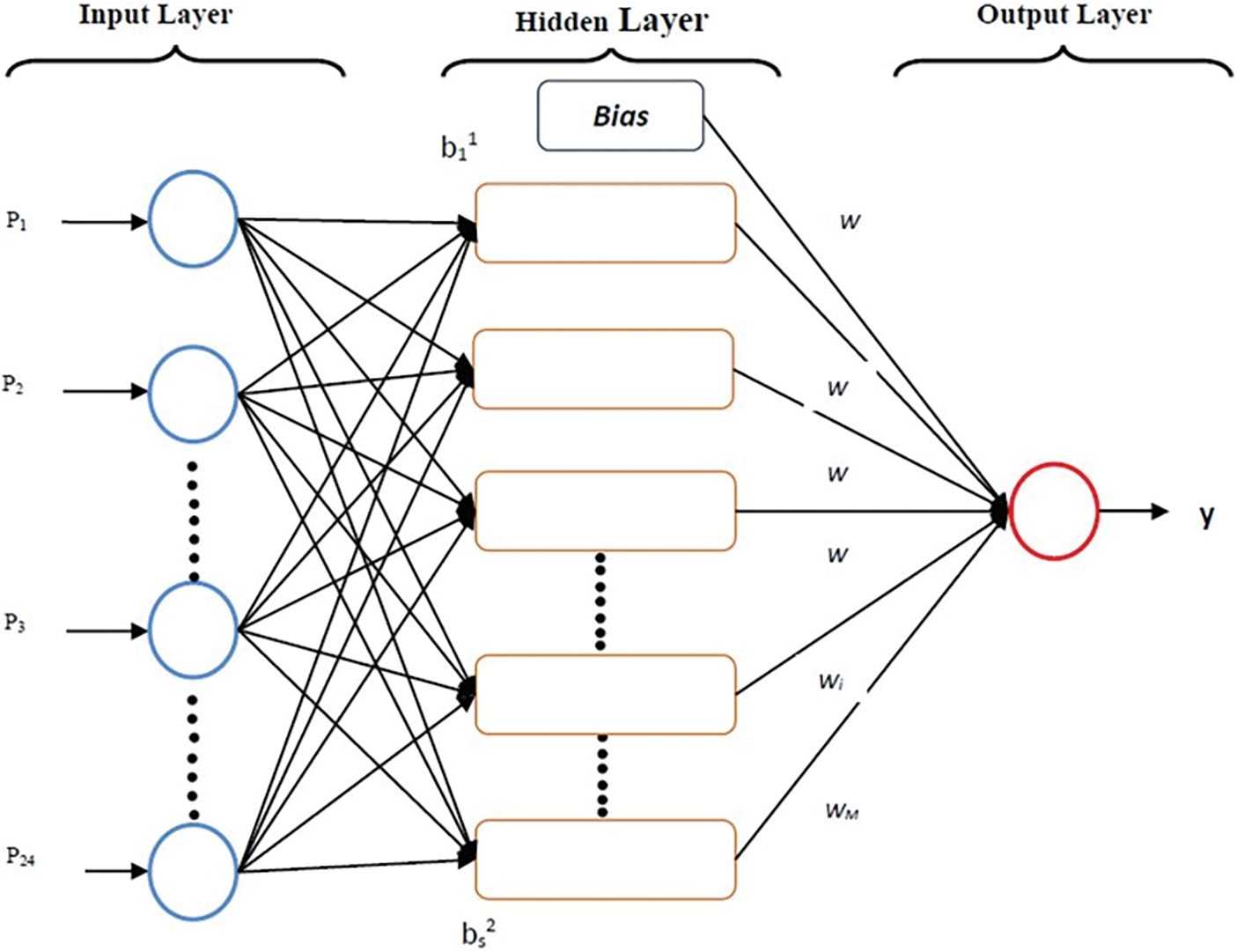
Figure 1: The building blocks of an ANN

The primary objective of this research work is to increase cultivated crops’ yield and instruct farmers about climatic factors and soil features that contribute to the fight against world hunger. In order to obtain temperature, N, P, and K for agricultural production in the Coimbatore districts of India, non-linear and complicated ANN relationships between several meteorological parameters were used. The Neural Network (NN) model is trained using the three training algorithms Levenberg-Marquardt (LM), Bayesian Regularization (BR), and SCG, and their prediction accuracy is compared. The LM training algorithm surpasses the SCG-BR method, according to a comparison of three training algorithms [18].

2.1 Levenberg-Marquardt

The LM algorithm constitutes a significant rationale for using this method to reduce the error function. For minimizing a non-linear process, the LM algorithm is a relatively efficient method. The algorithm incorporates many distinct factors, including output data, neuron weights, and error functions, which impact the model’s efficiency and success rate. The test function significantly influences the ideal values of these variables. The LM is quick and has a consistent convergence rate [19].

The Hessian matrix is predicted, and the gradient is computed using the formula below.

H=JkTJk(1)

g=JkTe(2)

In Eqs. (1) and (2), the Jk Jacobian matrix for kth input, ‘e’, is a vector of network errors containing first-order derivatives and mistakes concerning the weights and biases.

The following Eq. (3) gives the relationship for manipulative the LM, which is the grouping of the Guass Newton algorithm and the descent method:

Wk+1=Wk−[JkTJk+μI]−1JKTek(3)

where, I-identity matrix; Wk-current weight; Wk+1-next weight; ek+1-current total error; ek-last total error;

µ - combination coefficient.

It aims to combine the benefits of both approaches, inheriting the Gauss–Newton algorithm’s speed and the steepest descent method’s stability. When a step increases ek+1, the order coefficient “μ” is increased by a factor (β), and when a degree decreases ek+1, µ it is divided by “β”. Here, assumed = l0 in this study. The algorithm becomes the steepest descent when ‘μ’ is significant, whereas it becomes Gauss–Newton when ‘μ’ is small. The LM was used in this investigation with input neurons with no transfer function. In the hidden and output layers of the network, the logistic sigmoid transfer (login) and linear transfer (purelin) functions were applied as activation functions, respectively.

2.2 Scaled Conjugate Gradient

For better error minimization, the steepest descent technique is further modified to the next improved version called SCG, which provides better accuracy than the previous one [20]. This direction is referred to as the conjugate direction. Most SCG algorithms modify the step size after every iteration. This procedure, defined by Eq. (4), presents a negative gradient by beginning the steepest descent in the first iteration, and the weights are reviewed at each iteration (5).

p0=−g0(4)

xk+1=xk+αkgk(5)

Now, the step size is computed using ‘αk’, which is shown in Eq. (6)

Pk=−gk+βkPk−1(6)

where, p–search direction vector and g–gradient direction vector.

SCG can be divided into several types based on how the factor ‘βk’ is determined. In this paper, we applied the SCG, which combines the LM and CG, to calculate step size, as opposed to the CG approach, which solely uses the line search model. The SCG seeks to determine the direction of the performance function’s rapid decline while maintaining error minimization consideration. At every iteration, the step size is modified, and the step size is calculated by searching in the gradient direction. The step size is usually determined using the line search model. Because this line search is required in all rounds, the SCG descent techniques are time-consuming. The transfer function of the neurons in the input layer usually determines the step size. Eq. (7) is used to determine the ‘βk’ value, and Eq. (8) is used to find Pk+1 of the new search in the SCG.

βK=(gk+1|2−gk+1Tgk)gkTgk(7)

Pk+1=−gk+1+βkPk(8)

The algorithm’s success depends separately on each iteration’s user-updating design parameters. This is a considerable benefit over algorithm-based online searches.

2.3 Bayesian Regularization

Traditional back-propagation networks are less potent than BR-ANNs; therefore, they do not require as much cross-validation. By using ridge regression, the BR technique converts a non-linear regression into a “well-modelled” statistical probe. Regularization is performed in this method to enhance the network by optimizing the performance function F(ω). The performance function F() is the sum of the squares of the network weight errors (Ew) and the courts of the data errors (ED) [21].

F(ω)=αEW+βED(9)

EW=∑i=1nwi2(10)

ED=∑k=1nek2(11)

where Eqs. (9) and (10) are the objective function parameters, the network weights are represented as random variables in the BR framework, and the network weights and training set distribution are considered to have a Gaussian distribution. To define factors, Bayes’ theorem is utilized. Bayes’ theorem attempts to bridge the gap between two variables events, A and B, based on their prior marginal and later conditional probabilities, as shown in Eq. (12).

P(A∣B)=P(B∣A)P(A)P(B)(12)

If event B occurs, the conditional probability of event A is P(A|B), the conditional probability of event B is P(B|A), and the prior probability of event B is P(B). The performance function F(ω) must be minimized to produce the optimal weight values, equivalent to maximizing the probability function given by Eq. (13).

P(α,β∣D,M)=p(D∣α,β,M)P(α,β∣M)P(D∣M)(13)

where “α” and “β” are the factors that influence the value of F(ω), which is the M-specific NN style to be optimized; D-weight distribution; P(D|α, M)-probability function of D for given M; and P(α, β|M)-consistent prior density for the regularisation parameters. This method finds the optimal values for a given weight space. Later, the algorithm enters the LM phase, which involves executing Hessian matrix calculations and updating the weights to minimise the objective function’s value. If the fitness function’s convergence does not meet expectations, the algorithm predicts new values and repeats the procedure until convergence is achieved [22].

3  Proposed Methodology

The most widely used ML method for CYP is ANN. ANN mimics the human brain. One of ANN’s benefits is that it learns patterns from past datasets without computing the parameters statistically. It simulates the intricate, nonlinear connection between input and output. The information, hidden, and output layers are the structure of an ANN. The number of neurons in the input layer is comparable to the number of independent input variables; however, there is just one neuron in the output layer, which is the dependent. Production is the only output-dependent variable. There is a hidden layer sandwiched between the input and output layers. These three layers are all interconnected completely. The hidden layer transmits the signal from the input layer to the output layer.

The presented ANN model was created utilizing a modular NN with two hidden layers that could CYP output based on farm circumstances, social factors, and meteorological inputs. The Mean Square Error (MSE) and correlation of determination (R) are used to validate the data. As a result, numerous types of research in the literature implement ANN to ascertain how environmental variables and paddy crops relate to one another.

The ANN designs for CYP output were created using matrix laboratory (MATLAB). The CY was the dependent variable in the ANN design, which had one hidden layer. The characteristics of weather forecasting characteristics were included in the input parameters of the ANN model. For every input and output parameter, time series data were separated into training (70%), validation (15%), and testing (15%). The training process began with the choice of training algorithms. When compared to the experimental constraints, lower MSE values and R values closer to “1” yield better predictions; Eqs. (14) and (15) represent the R and MSE parameters, respectively [23]. The relation between R and MSE is described in Eqs. (14) and (15), and it is computed for the entire condition of ANN.

R=N∑xy−(∑x)(∑y)(N∑x2−(∑x)2)(N∑y2−(∑y)2)(14)

MSE=∑i=1N|xi−yi|N(15)

where, x–Experimental value; Y–the predicted value; N–number of observations.

The formula for the non-linear relationship that was represented here is given in Eq. (16)

CropYield=φ(Climaticfactor,soilnutrients)(16)

where ‘φ’ is a non-linear function that connects CY, soil nutrients, and environmental conditions [24]. Depending on data availability, the connection is developed on a regional basis for harvesting seasons.

The data set is preprocessed for feature identification and interpretation, missing value treatment, and outlier treatment before applying the feature selection algorithm. The data’s quality determined the output’s quality. This collection includes measurements for each attribute. Every attribute in this collection has its measures. The dataset has been rescaled to get an accurate prediction, and the dataset has been rescaled using Eq. (17).

X′=xi−min(x)max(x)−min(x)(17)

where X′ is the rescaled value of X, X is the attribute value, min(X) is the attribute value’s minimum, and max(X) is the attribute value’s maximum.

4  Experimental Study

The district of Coimbatore covers a total area of 4723 square kilometres. It is situated between the latitudes 10°10′ and 11°30′ north and the longitudes 76°40′ and 77°30′ east. The district headquarters are in the region’s north-central section. The area is bordered on the west by the Western Gates, on the north by the Nilgiris, and on the south by the Anaimalai and Palani hills. It is divided into different regions, as depicted in Fig. 2. The Western Ghats surround Coimbatore. The Noyyal river, which passes through the city, defines Coimbatore’s southern limit. The city is located in the Noyyal River basin and has an enormous reservoir system nourished by rainwater and the river. The city of Coimbatore, as well as the district’s eastern portion, is primarily dry. The state’s western border is marked by the Palghat Gap, a western pass into Kerala [25].

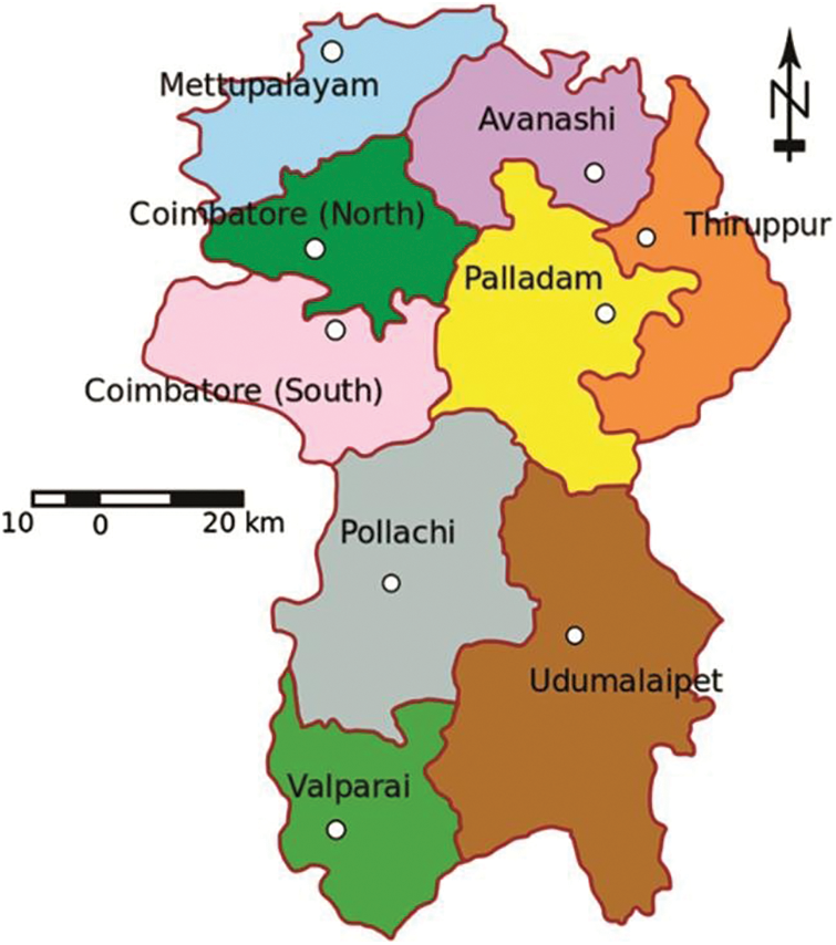
Figure 2: Coimbatore region map of the study area

The district’s main soil types include deep red soil and black dirt. They comprise 35.9% of the total area, followed by relatively deep black (15.4%) and shallow red (13.4%). (18.6%) of the soil is predominantly black, making it perfect for cotton cultivation. The medium-to-deep-red calcareous soils of Pollachi taluk are well-known. Small sections of alluvial soil can be found sideways in the Noyyal river, mainly in the higher stages [26].

In April and May, the average temperature is 29.12°C. During the winter months of October to March, a mean average temperature of 25.34°C [27]. The average rainfall in the district is between 650 and 700 mm. The northeast monsoon gets the most rainfall, accounting for 44% of total rainfall, followed by the southwest monsoon with 37%, whereas summer rainfall is around 17%. Climate and soil nutrient data were obtained from the Tamil Nadu Department of Economics and Statistics, and soil health cards were accepted from the Tamil Nadu Department of Agriculture and Farmers Welfare. The corresponding CY data were obtained from the International Crop Research Institute.

NN was used for different environmental conditions based on the available data to set up the relationship indicated by CY = 1(N, P, K). As previously stated, the NN analysis was carried out using ANN [28].

ANN was widely applied by many researchers to estimate diverse agricultural yields, as indicated in Section 1. Researchers took into account multiple factors, such as maximum and minimum temperatures, average rainfall, humidity, climate, weather, land types, chemical fertilizer types, type of soil, the structure of the soil, composition level of the soil, moisture content present in the soil, consistency of the soil, and texture of the soil. However, many models, together with linear, NN, and penalized regression models, have been used for CYP on India’s west coast [29,30].

5  Results and Discussions

The below visual represents the R values for five crops in the Coimbatore region using the LM, BR, and SCG for rice, sorghum, groundnut, maize, and chickpea production. It clearly shows that the ANN-based LM training procedure has provided a reasonable evaluation of rice yield. For the essential scenarios, training, validation, and testing. The R values are 0.9, nearer to one. Figs. 3a, 3b, 4c, 4d, 5e, 5f, 6g and 6h depict the R of training, validation, testing, and all values for rice and groundnut using the LM. In addition, Fig. 7i shows the process’s computational efficiency for rice crops. In 7 epochs, the trained NN using the LM method produces a better outcome when compared to the BR, SCG, and LM, giving it a good speed of response. As a result, it is more computationally efficient.

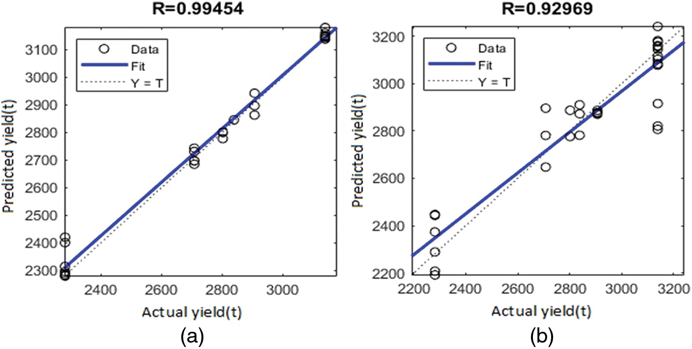
Figure 3: Regression plot showing R using LM for rice crop for (a) training, (b) validation

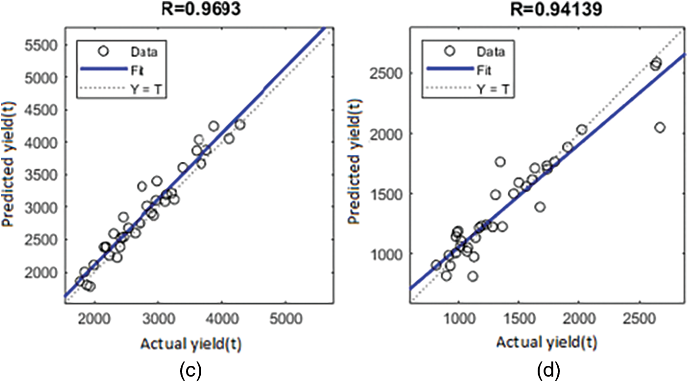
Figure 4: Regression plot showing R using LM for rice crop for (c) test graph (d) all graph

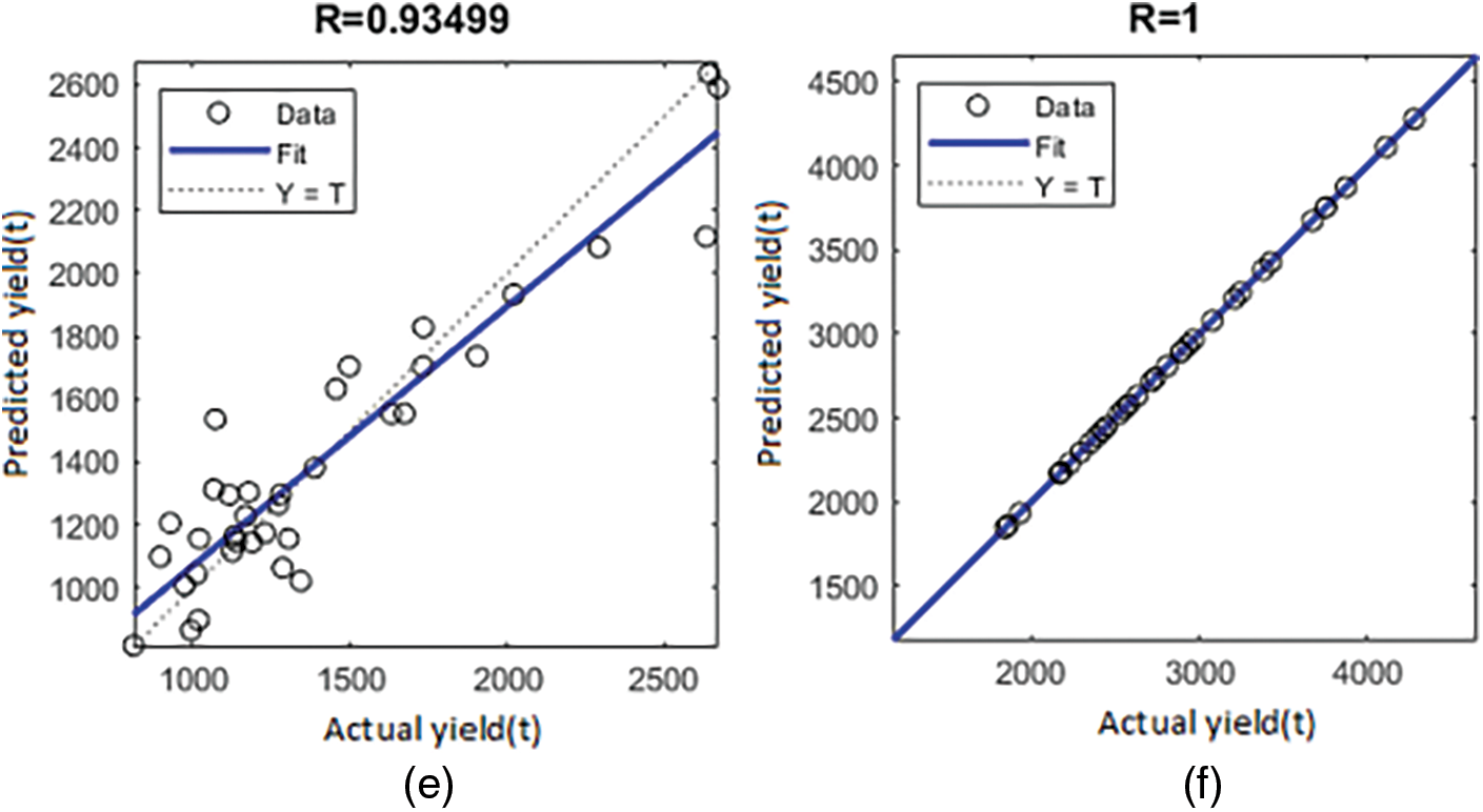
Figure 5: Regression plot showing R for groundnut using LM (e) training (f) validation

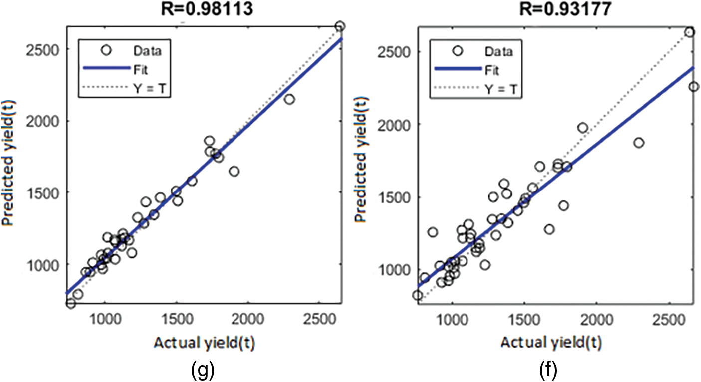
Figure 6: Regression plot showing R for groundnut using LM (g) test graph (h) all graph

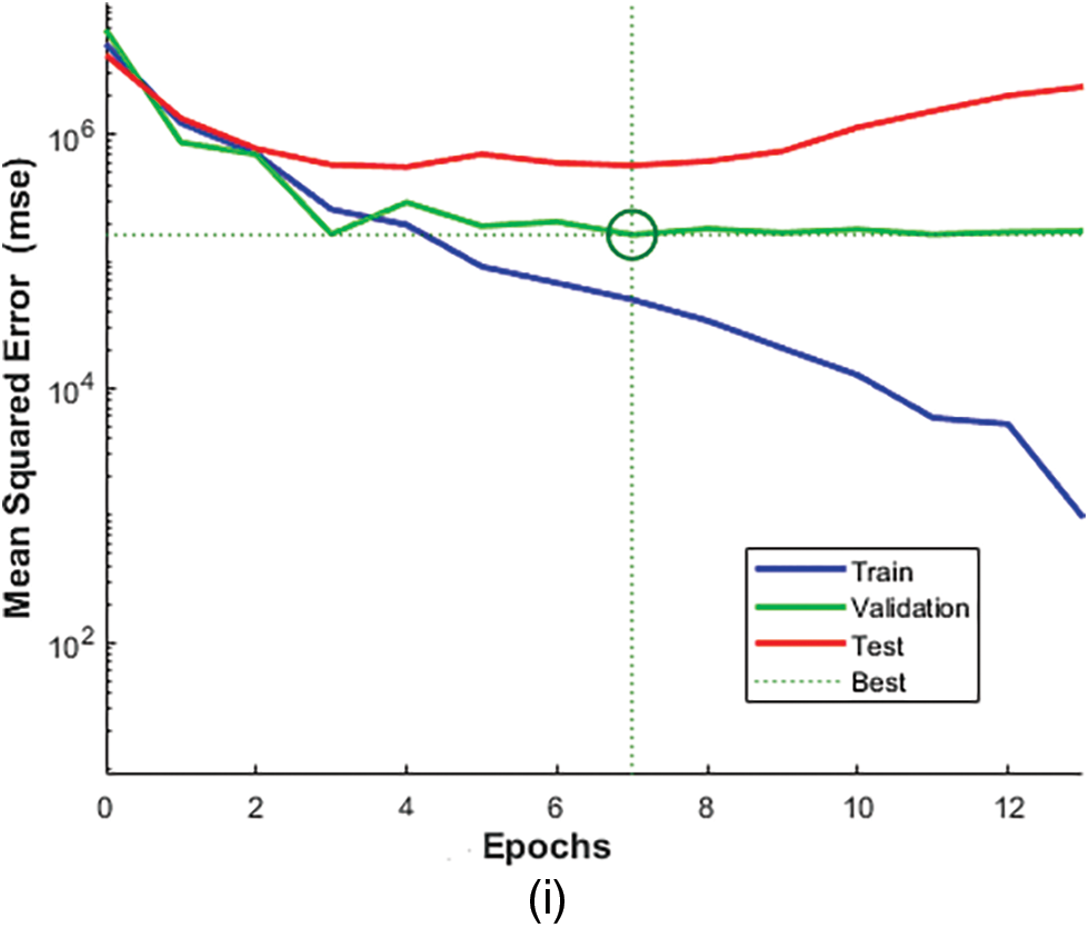
Figure 7: Regression plot showing R for groundnut using LM (i) network validation performance graph for LM for rice crop

Furthermore, Figs. 8a, 8b, 9c, 9d, 10e, 10f, 11g, 11h, 12i and 12j show the R obtained for rice, groundnut, maize, chickpea, and sorghum CY applied using the BR and SCG algorithms. The R values are substantially lower than those obtained using the LM (R = 0.99454 and 0.92969 for training and validation, respectively). As a result, the LM beats both the BR and SCG. Much more research comparing the LM method to other training algorithms has reached the same conclusion. Although the BR and SCG aim to minimize the MSE and have the fastest convergence, the LM ANN result is better regarding predictive ability.

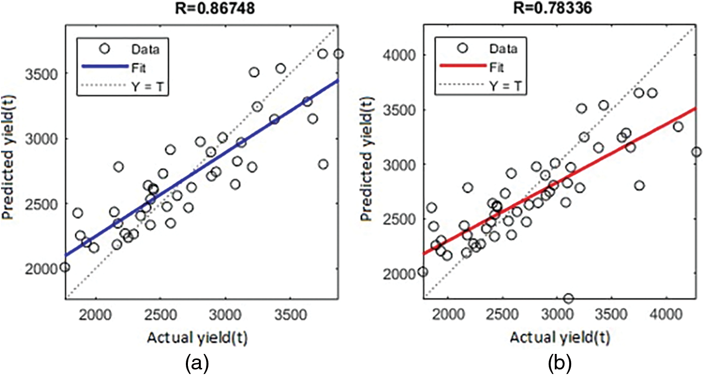
Figure 8: Regression plot showing the R for rice crop (a) validation-BR (b) validation-SCG

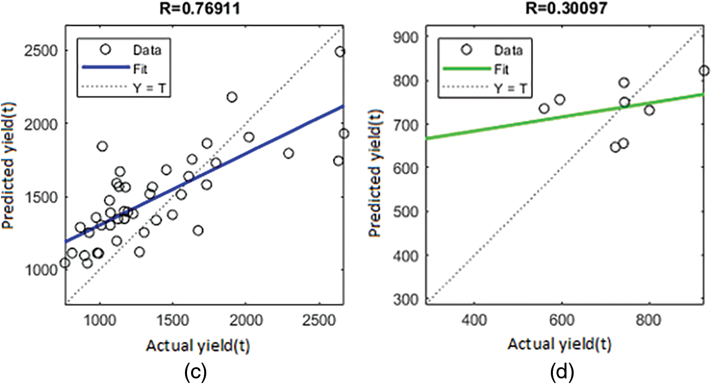
Figure 9: Regression plot showing the R for groundnut crop (c) validation-BR (d) validation-SCG

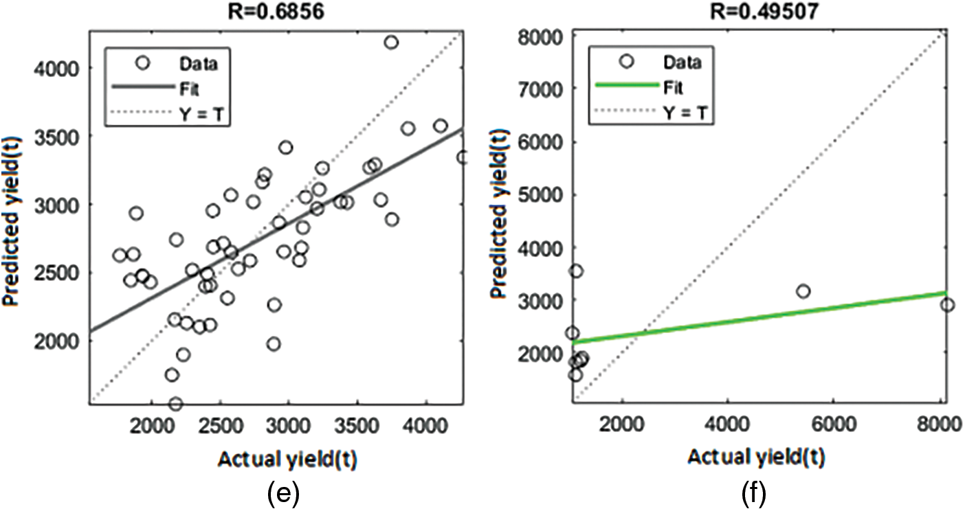
Figure 10: Regression plot showing the R for maize (e) validation-BR (f) validation-SCG

Figure 11: Regression plot showing the R for chickpea (g) validation-BR (h) validation-SCG

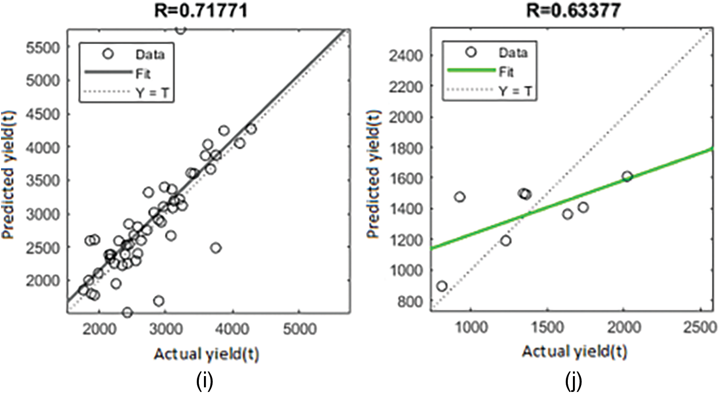
Figure 12: Regression plot showing the R for sorghum (i) validation-BR (j) validation-SCG

The R-value for crops in Coimbatore districts was assessed using BR and SCG. The values of R scope in the LM are clearly understood to be nearly one. It would be fascinating to look into the outcomes of the Eq. (9) relationship. As previously stated, the analysis shows five crops in the Coimbatore district. Figs. 3 to 7 show the R for crop rice and groundnut in the LM (Fig. 8 to 12). For the BR and SCG, similar findings are attained in the indicated relationships as in Eq. (16).

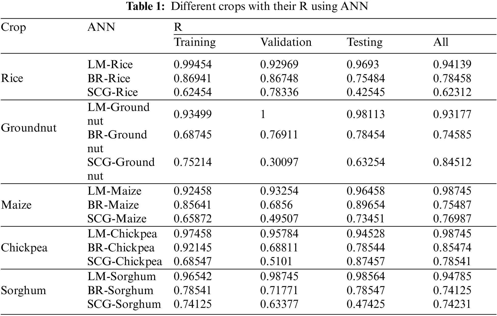
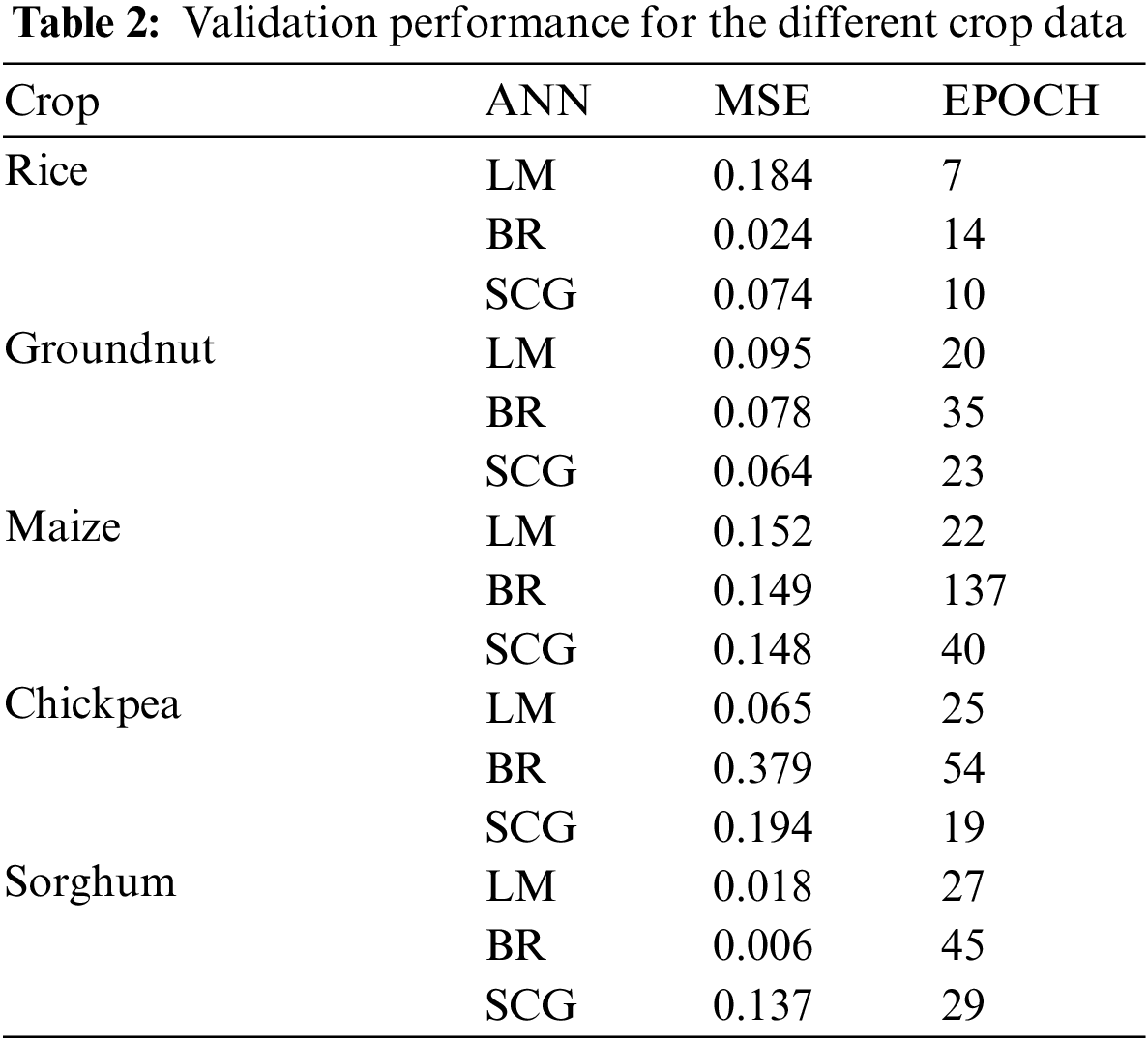
According to the results, the LM method performs better than the other training algorithms. Table 1 depicts the performance of the ANN trained to find out the correlations among climatic parameters; the version of the ANN introduced to find out the correlations among climatic parameters (temperature, N, P, and K) for different CPs applied with training measures (LM, BR, and SCG). The LM outperformed the other training algorithms in terms of R. Other algorithms, on the other hand, fared relatively well in determining the relationship between climatic features, N, P, and K for CYP, with acceptable R values. The validation results of these training algorithms used to determine the link between climatic conditions and CYs are shown in Table 2. In terms of validation performance, three training algorithms performed well, with decreased MSE values. Regarding the number of epochs and processing time, however, LM and SCG have fared well with fewer epochs and lesser processing times. The BR has a more significant number of epochs. As a result, with MSE closer to ‘0’ in fewer epochs and good R, the LM helped obtain the relation between the climatic component’s temperature, N, P, and K for CP.

All of the references declared earlier came to the same key conclusion: because the prediction relies on climate data and soil nutrients, there is constantly an error threshold in the forecast. Many investigations have come to the same conclusion. Several factors, including changing climate, regional distribution of weather data, and data quality, can all contribute to uncertainty. As indicated in Section 1, ANN was commonly functional by many researchers to focus on various CYPs. Researchers conducted a similar investigation with more factors. They considered maximum and minimum temperatures, average rainfall, humidity, weather, land types, chemical fertilizer forms, soil nature, and soil structure. Despite all of the work, the prediction is still within acceptable bounds. Farmers would not be interested in an accurate CYP estimate, but they would be glad to accept a reasonable forecast. Surprisingly, several parts of Coimbatore have been subjected to the same research. The prediction is consistent. However, the R is in the range of 0.6–0.8. As a result, the forecast has a similar error threshold. As a result, more studies should be done for a more accurate prediction model, whereas the existing model is used as a reference. As shown in Fig. 13, an evaluation graph was plotted between three algorithms for distinct crop data sets, and it is clear that the LM has a lower epoch value (7), which shows high precision output at a down computational time.

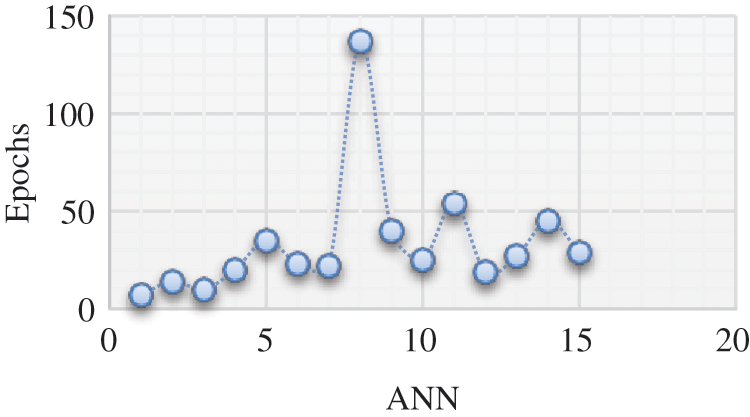
Figure 13: Validation performance of the different algorithms for crop data

Three different training algorithms—the LM, the BR, and the SCG—are used to train the final NN model, and their comparison is made. The developed ANN models’ efficacy was assessed using R and MSE as performance metrics. According to the findings, LM outperforms other algorithms in discovering correlations between input variables and CY.

When evaluated side by side, ANNs have several advantages over statistical models. ANN models make no assumptions regarding the distribution or characteristics of the data. ANNs are more useful in practical applications as a result. Additionally, ANN models do not require any testing hypotheses, in contrast to some statistical models that do—enhancing model transparency and facilitating information extraction from trained ANNs in a way that offers a thorough grasp of the relationship between model inputs and outcomes.

6  Conclusions and Future Work

The objective of this research work is to demonstrate the predictive abilities of Levenberg–Marquardt (LM), Bayesian Regularization (BR), and Scaled Conjugate Gradient (SCG) training algorithms. The ability to predict reflective thinking in the data was implemented with three different backpropagation algorithms. The best model was examined as LM by looking at the highest correlation rate and the shortest computational time with a satisfied MSE value. Relationships between several climatic parameters that are non-linear and complex (ANN) were used to acquire temperature, N, P, and K for crop production in the Coimbatore districts of India. A comparison of training algorithms reveals that the LM outperforms the SCG-BR.

The BR and SCG, on the other hand, have sent acceptable results. As a result, the LM is applied to future CYP at a lower computation cost. These connection coefficients, however, are suitable in the context of substantial weather conditions, according to the research. As a result, it can be inferred that the CY temperature, NPK, and meteorological conditions have a good relationship. As a result, it is stated that ongoing climate change substantially impacts CY. More crucially, the study includes these nonlinear interactions. As a result, reverse computations are possible in the event of future climatic data. To extract future climate data, ANN is repeated to obtain the related CY data using different climate models. As a result, planners and authorities need to pay close attention to this prognosis in order to prepare for long-term sustainable cropping patterns. On the other hand, farmers do not expect accurate forecasts but rather somewhat realistic ones.

Furthermore, the models are used to design adequate plans for food sustainability in extreme climate events. However, these models are reinforced further by integrating more climate and soil features and implementing more deep-learning algorithms. It would also be interesting to examine the correlations between other critical variables, such as agricultural, industrial advances and new crop variations that control some climate excesses, as well as the adverse effects of multiple pests on crop productivity.

Funding Statement: The authors received no specific funding for this study.

Conflicts of Interest: The authors declare that they have no conflicts of interest to report regarding the present study.

References

1. R. Panahabadi, A. Ahmadikhah, S. McKee Lauren, K. P. Ingvarsson and N. Farrokhi Naser, “Genome-wide association mapping of mixed linkage (1,3;1,4)-β-glucan and starch contents in rice whole grain,” Frontiers in Plant Science, vol. 12, no. 665745, pp. 1–14, 2021. [Google Scholar]

2. A. Ahmadikhah, N. Bagheri, N. Farrokhi and R. Panhabadi, “Genome-wide association study (GWAS) of germination and post-germination related seedling traits in rice,” Euphytica, vol. 218, no. 8, pp. 1–21, 2022. [Google Scholar]

3. P. Dilli, B. Hendrik, W. Allardde, J. Sander, O. Sjoukje et al., “Machine learning for large-scale crop yield forecasting,” Agricultural Systems, vol. 187, no. 1, pp. 1–13, 2021. [Google Scholar]

4. K. Palanivel and C. Surianarayanan, “An approach for prediction of crop yield using machine learning and big data techniques,” International Journal of Computer Engineering and Technology, vol. 10, no. 3, pp. 110–118, 2019. [Google Scholar]

5. P. M. Gopal and R. Bhargavi, “A novel approach for efficient crop yield prediction,” Computers and Electronics in Agriculture, vol. 165, no. 1, pp. 1–9, 2019. [Google Scholar]

6. N. Shima, M. Sachin, M. Ezgi, K. Stevan, C. J. May et al., “Machine learning techniques for mitoses classification,” Computerized Medical Imaging and Graphics, vol. 87, no. 1, pp. 1–8, 2021. [Google Scholar]

7. A. G. Sanchez, J. F. Solis and W. O. Bustamante, “Predictive ability of machine learning methods for massive crop yield prediction,” Spanish Journal of Agricultural Research, vol. 12, no. 2, pp. 313–328, 2014. [Google Scholar]

8. N. Rale, R. Solanki, D. Bein, J. A. Vasko and W. Bein, “Prediction of crop cultivation,” in Proc. of IEEE 9th Annual Computing and Communication Workshop and Conf., Las Vegas, NV, USA, pp. 227–232, 2019. [Google Scholar]

9. K. Abrougui, K. Gabsi, B. Mercatoris, C. Khemis, R. Amami et al., “Prediction of organic potato yield using tillage systems and soil properties by artificial neural network (ANN) and multiple linear regressions (MLR),” Soil and Tillage Research, vol. 190, no. 5, pp. 202–208, 2019. [Google Scholar]

10. X. E. Pantazi, D. Moshou, T. Alexandridis, R. L. Whetton and A. M. Mouazen, “Wheat yield prediction using machine learning and advanced sensing techniques,” Computers and Electronics in Agriculture, vol. 121, no. 1, pp. 57–65, 2016. [Google Scholar]

11. S. V. Joshua, A. S. M. Priyadharson, R. Kannadasan, A. A. Khan, W. Lawanont et al., “Crop yield prediction using machine learning approaches on a wide spectrum,” Computers, Materials & Continua, vol. 72, no. 3, pp. 5663–5679, 2022. [Google Scholar]

12. A. Chlingaryan, S. Sukkarieh and B. Whelan, “Machine learning approaches for crop yield prediction and nitrogen status estimation in precision agriculture: A review,” Computers and Electronics in Agriculture, vol. 151, no. 1, pp. 61–69, 2018. [Google Scholar]

13. M. M. Saritas and A. Yasar, “Performance analysis of ANN and Naive Bayes classification algorithm for data classification,” International Journal of Intelligent Systems and Applications in Engineering, vol. 7, no. 2, pp. 88–91, 2019. [Google Scholar]

14. A. Abraham, “Meta-learning evolutionary artificial neural networks,” Neurocomputing, vol. 56, no. 3, pp. 1–38, 2010. [Google Scholar]

15. S. Uddin, A. Khan, M. E. Hossain and M. A. Moni, “Comparing different supervised machine learning algorithms for disease prediction,” BMC Medical Informatics and Decision Making, vol. 19, no. 1, pp. 1–16, 2019. [Google Scholar]

16. M. Nikou, G. Mansourfar and J. Bagherzadeh, “Stock price prediction using deep learning algorithm and its comparison with machine learning algorithms,” Intelligent Systems in Accounting, Finance and Management, vol. 26, no. 6, pp. 164–174, 2019. [Google Scholar]

17. S. Bharati, M. A. Rahman, P. Podder, M. R. A. Robel and N. Gandhi, “Comparative performance analysis of neural network base training algorithm and neuro-fuzzy system with SOM for the purpose of prediction of the features of superconductors,” in Proc. of Int. Conf. on Intelligent Systems Design and Applications, Auburn, WA, USA, pp. 69–79, 2019. [Google Scholar]

18. M. Kayri, “Predictive abilities of bayesian regularization and Levenberg-Marquardt algorithms in artificial neural networks: A comparative empirical study on social data,” Mathematical and Computational Applications, vol. 21, no. 2, pp. 1–20, 2016. [Google Scholar]

19. R. Parmar, M. Shah and M. G. Shah, “A comparative study on different ANN techniques in wind speed forecasting for generation of electricity,” IOSR Journal of Electrical and Electronics Engineering, vol. 12, no. 1, pp. 19–26, 2017. [Google Scholar]

20. A. Suliman and B. S. Omaro, “Applying Bayesian regularization for acceleration of Levenberg-Marquardt based neural network training,” International Journal of Interactive Multimedia and Artificial Intelligence, vol. 5, no. 1, pp. 68–72, 2018. [Google Scholar]

21. J. Cao, Z. Zhang, F. Tao, L. Zhang, Y. Luo et al., “Integrating multi-source data for rice yield prediction across China using machine learning and deep learning approaches,” Agricultural and Forest Meteorology, vol. 297, no. 1, pp. 108275, 2021. [Google Scholar]

22. R. Bala and D. Kumar, “Classification using ANN: A review,” International Journal of Computational Intelligence Research, vol. 13, no. 7, pp. 1811–1820, 2017. [Google Scholar]

23. C. Karan and K. Farhana, “Prediction of crop yield using machine learning,” International Journal of Engineering Applied Sciences and Technology, vol. 4, no. 4, pp. 153–156, 2020. [Google Scholar]

24. S. Baruah, A. Kumaraperumal, B. Kannan, K. P. Ragunath and M. R. Backiyavathy, “Soil erodibility estimation and its correlation with soil properties in Coimbatore district,” International Journal of Chemical Studies, vol. 7, no. 3, pp. 3327–3332, 2019. [Google Scholar]

25. B. Guillaume, G. Konstantin, B. Luca and S. Sokrat, “Responses of soil properties and crop yields to different inorganic and organic amendments in a Swiss conventional farming system,” Agriculture, Ecosystems & Environment, vol. 23, no. 1, pp. 116–126, 2016. [Google Scholar]

26. K. Kandiannan, K. Chandaragiri, N. Sankaran, T. N. Balasubramanian and C. Kailasam, “Crop weather model for turmeric yield forecasting for Coimbatore district, Tamil Nadu, India,” Agricultural and Forest Meteorology, vol. 112, no. 1, pp. 133–137, 2002. [Google Scholar]

27. R. Ben Ayed and M. Hanana, “Artificial intelligence to improve the food and agriculture sector,” Journal of Food Quality, vol. 2021, no. 1, pp. 1–7, 2021. [Google Scholar]

28. V. Amaratunga, L. Wickramasinghe, A. Perera, J. Jayasinghe and U. Rathnayake, “Artificial neural network to estimate the paddy yield prediction using climatic data,” Mathematical Problems in Engineering, vol. 2020, no. 1, pp. 1–11, 2020. [Google Scholar]

29. P. Ekanayake, W. Rankothge, R. Weliwatta and J. W. Jayasinghe, “Machine learning modelling of the relationship between weather and paddy yield in Sri Lanka,” Journal of Mathematics, vol. 2021, no. 1, pp. 1–14, 2021. [Google Scholar]

30. A. Mustafa Hilal, H. Alsolai, F. N. Al-Wesabi, M. Abdullah Al-Hagery, M. Ahmed Hamza et al., “Artificial intelligence based optimal functional link neural network for financial data science,” Computers, Materials & Continua, vol. 70, no. 3, pp. 6289–6304, 2022. [Google Scholar]