Enhanced Tunicate Swarm Optimization with Transfer Learning Enabled Medical Image Analysis System

1  Introduction

Medical imaging is a significant diagnostic tool for many diseases. In 1895, roentgen found that x-rays can non-invasively look into the human body and x-ray radiography is the first diagnostic image modality soon after [1]. Thereafter, several imaging modalities are developed, with magnetic resonance imaging (MRI), computed tomography, positron emission tomography and ultrasound among the typically utilized, and increasingly complicated imaging process formulated [2,3]. Image information had a main role in making decisions at numerous phases in the process of patient care, which includes staging, detection, treatment response assessment, surgeries, monitoring of disease recurrence, and characterization in addition to guiding radiation therapy and interventional process [4]. The images for a given victim case rise drastically from some 2D images to hundreds with 3D images and thousands with 4D imaging. There will be a rise in the number of image datasets to be interpreted by applying multi-modality imaging [5–7]. The increasing workload finds it tough for physicians and radiologists to preserve workflow efficiency when using all the available imaging data for enhancing patient care and accuracy [8–10]. With the advancements in computational techniques and machine learning (ML) in recent years, the need of formulating computerized techniques for assisting radiologists in diagnosis and image analysis was recognized as a significant area of research and studies in medical imaging [11].

Transfer learning (TL) is an application of artificial intelligence that depends on pretrained learning that offers enrichment in the rate of diagnosis and accuracy using medical imaging [12]. There were robust market demands and public engrossment that pushes the rapid production of these diagnostic products [13]. The techniques of TL render structure for using formerly obtained knowledge to solve new but related problems a lot more effectively and promptly through AI. The TL techniques have the feature of fine-tuning the method based on the formerly trained dataset, permitting them to alter their provided input layers. This feature made them powerful tools to catalogue and detects the pattern of diseases. Moreover, the exposed features do not process by medical experts, but to some extent by the series they have trained from the inputted dataset [14]. Contrary to this, DL techniques have reached significant and amazing deviations to medical engineering, with their discoveries in the domain of pattern recognition, image captioning and computer vision [15].

Gaur et al. [16] examined a practical solution for detecting COVID19 in chest X-rays (CXR) but typical individuals in normal and compressed by Viral Pneumonia using DCNN. During this case, 3 pre-trained CNN techniques (InceptionV3, EfficientNetB0, and VGG16) can be estimated with transfer learning (TL). The rationale to select these particular methods is their balancing of accurateness and efficacy with several parameters appropriate to the mobile application. Chouhan et al. [17] purposed of this analysis is for simplifying the pneumonia recognition procedure for experts and novices. The authors propose a new DL structure for the recognition of pneumonia utilizing the model of TL. In this manner, the feature in images can be extracted utilizing distinct NN algorithms pre-trained on ImageNet that are provided as to classification to predictive.

Arora et al. [18] purposed for identifying COVID19 with DL approaches utilizing lung CT-SCAN image. For enhancing lung CT scan efficacy, a super-residual dense NN is executed. To mark COVID19 as positive/negative to enhance CT scans, current pre-training approaches like ResNet50, XceptionNet, MobileNet, VGG16, InceptionV3, and DenseNet are utilized. Ali et al. [19] examined a DCNN technique dependent upon the DL algorithm for the correct classifier betwixt malignant and benign skin lesions. During the pre-processed, the authors initially execute a filter or kernel for removing noise and artefacts; secondarily, normalise the input images and extract features which use to accurate classifier; and at last, data augmentation enhances the count of images which enhances the rate of classifier accuracy.

Al-Rakhami et al. [20] introduced an integrated structure of CNN and recurrent neural network (RNN) for diagnosing COVID19 in CXR. The deep transfer approaches utilized in this experiment are InceptionV3, VGG19, Inception-ResNetV2 and DenseNet121. CNN has been utilized for extracting difficult features in instances and classifying them utilizing RNN. The VGG19-RNN infrastructure attained an optimum performance betwixt every network concerning accuracy. Lastly, the Gradient-weighted Class Activation Mapping (Grad-CAM) has been utilized for visualizing class-specific regions of images that are responsible for decision-making. The purpose of the analysis is to evaluate the efficiency of recent CNN infrastructures presented in recent times for medicinal image classifiers (Apostolopoulos et al. [21]). Especially, the process named TL with executed. With TL, the recognition of several abnormalities from smaller medicinal image databases is the reachable target, frequently yielding remarkable outcomes.

This study develops an Enhanced Tunicate Swarm Optimization with Transfer Learning Enabled Medical Image Analysis System (ETSOTL-MIAS). The ETSOTL-MIAS technique involves the Chan Vese segmentation technique to identify the affected regions in the medical image. For feature extraction purposes, the ETSOTL-MIAS technique designs a modified DarkNet-53 model. To avoid the manual hyperparameter adjustment process, the ETSOTL-MIAS technique exploits the ETSO algorithm. Finally, the classification of medical images takes place by random forest (RF) classifier. The performance validation of the ETSOTL-MIAS technique is tested on a benchmark medical image database.

The rest of the paper is organized as follows: Section 2 offers the proposed model and Section 3 discusses the experimental analysis. Finally, Section 4 concludes the study.

2  The Proposed Model

In this study, we have developed a new ETSOTL-MIAS technique for the identification and classification of bone cancer on medical imaging. It comprises Chan Vese segmentation, modified DarkNet-53 feature extraction, ETSO-based hyperparameter optimization, and RF classification. The ETSOTL-MIAS technique involved the design of the Chan Vese segmentation technique to identify the affected regions in the medical image. For feature extraction purposes, the ETSOTL-MIAS technique designs a modified DarkNet-53 model. To avoid the manual hyperparameter adjustment process, the ETSOTL-MIAS technique exploits the ETSO algorithm. Finally, the classification of medical images takes place by the RF classifier. Fig. 1 defines the block diagram of the ETSOTL-MIAS approach.

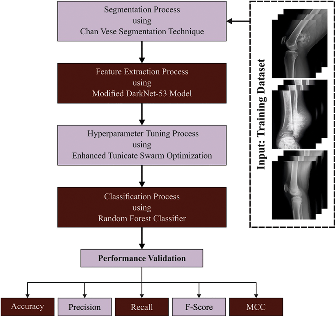
Figure 1: Block diagram of ETSOTL-MIAS system

2.1 Image Segmentation

The ETSOTL-MIAS technique involved the design of the Chan Vese segmentation technique. While segmenting images to define the bite-marked region, the Chan Vese technique can be exploited for the pre-processed image [22].

Assume f(x)=(x1, x2)∈Ω⊂Rt2 signifies the input image that must be segmented. The generalized image segmentation problems with the Mumford-Shah image are given as follows:

min μH1(C)+λ∫Ω(f−u)2dx+∫Ω\C|∇u|2dx,(1)

Now, C indicates the edge set, u represents the differentiable function on Ω\C, H1 indicates the 1D Hausdorff measure, ∇u=(uχ1tuχ2) represents the gradient operator, |⋅| signifies the L2 norm and variable μ>0tλ>0.

In Eq. (1), consider that C indicates the closed curve, the 1D Hausdorff measure of C gets curve length and it is formulated by:

argminu, Cμ length (C)+λ∫Ω(f−u)2dx+∫Ω\C|∇u|2dx.(2)

Consider that the function:

u(x)={c12 if x∈Cc22 if x∉C ,

Then obtain the succeeding model:

argminc1,c2,Cμlength(C)+vArea(C)+λ1∫x∈C|f−c1|2dx+λ2∫x∉C|f−c2|2dxt(3)

From the expression, length (C) represents the length of curve C, Area (C) characterizes the area inside C, and variable μ>0, v>0,λ1>0,λ2>0.  Eq. (3) is called as Chan-Vese image segmentation technique. The objective is to determine the optimum u-fitting f by minimizing the aforementioned energy function. In Eq. (3), the first term characterizes the regularity by the curve length, the second term-penalize the enclosed area of C for controlling its size, and the third and fourth terms penalize discrepancy amongst the input image f and the piecewise constant function u.

2.2 Feature Extraction

To produce a set of feature vectors, a modified DarkNet-53 model is used [23]. It integrates the residual networks with deep residual architecture. It encompasses 1×1 and 3×3 convolution layer and residual block which can be formulated by Eq. (4):

amn=∑j∈Xiajn−1∗yjmn+zmn(4)

From the expression, the input image is twisted by the convolution kernel for producing m separate feature map amn that is characterized in n layers by m feature maps, ∗ denotes the convolution function. The feature vector of the image is denoted as Xi and the j component of the m convolutional kernel in n layers can be characterized as yjn.

Next, the main layer is the batch normalization (BN) layer.

aout=∝(amn−∂)ω2+ϕ+γ(5)

In Eq. (5), the scaling factor is characterized as ∝, the mean of each output can be denoted as ∂, the input variance can be indicated as ω, ϕ shows the constant offset characterized by γ, and the convolution computation outcome can be represented as aout. The outcome of BN is represented as aoui. The output is normalized through BN corresponding to the similar distribution of the coefficient of the similar batch of eigenvalues. Later, it has the convolution layer that could speed up the convergence rate and avoid avoiding overfitting. The subsequent layer is called the activation layer. In this work, a leaky ReLU layer can be added as an activation function:

χj={yj′ if aout≥0yibi, if aoui<0(6)

In Eq. (6), the input values are represented as yj, the activation value can be indicated as χj, and the fixed parameter in the range (1,+∞) can be represented as bj. Another significant layer is the pooling layer. In the network, this layer is used for weight downsampling. Besides, max -the pooling layer is applied. At last, every weight is integrated with one layer through the 1D array is termed a feature. Finally, this extracted feature was categorized in the output layer. The depth of these models is 53, the size is 155 MB, the number of variables is 41.6 million, and the input size of an image is 256-by-256.

The ETSO algorithm is derived for the hyperparameter adjustment process. Tunicate can discover the food source location in the sea [24]. Jet propulsion and swarm intelligence are the 2 characteristics of tunicate deployed for discovering the food resource. Tunicate must satisfy 3 conditions such as “avoid the conflicts between search agents, the movement towards the position of best search agent and remain close to the best search agent” to precisely model the characteristics of jet propulsion.

For avoiding conflicts amongst searching agents, vector B→ is deployed for calculating the novel location of the searching agent as follows:

B→=M→G→(7)

M→=C2+C3−F→(8)

F→=2.C1(9)

In Eqs. (8) and (9), M→ represent gravitational force and F→ stands for advection of water flow in the sea, C1, C2, and C3 show the arbitrary integers within [0,1]. G→ indicates social forces amongst searching agents. The vector G→ is calculated as given in Eq. (10), in which xmax and xmin indicate the subordinate and initial speed to make social interaction.

G→=[Xmin+C1.Xmax−Xmin](10)

The searching agent tends to shift towards a better-neighbouring direction afterwards avoiding the conflicts among neighbours, in which, X→D indicates the distance between the food source and search agent, F¯P indicates the food source location, x indicates the existing iteration, X¯p(y) shows the location of tunicate and rand denotes the arbitrary number within [0,1].

X→D=|F¯P−rand.X¯p(y)(11)

The search agent sustains its location to better search agent, while, x¯(y1) indicates the updated location of tunicate based on the food source location of F¯P as follows:

x¯p(y)={F¯P+B→.X→D if rand≥0.5F¯P−B→.X→D if rand<0.5(12)

To stimulate the swarming behaviour of tunicate, the initial optimum solution is stored and it can be mathematically expressed as follows:

xp(y1+1)=x→p(y)+xp(y→+1)2+C1(13)

The ETSO algorithm is designed by the use of the oppositional-based learning (OBL) concept. The OBL is an optimization approach utilized for improving the diversity of optimization techniques and improving its attained solution. Generally, the optimization algorithm starts its step towards an optimum solution by first producing a set of solutions randomly. But this attained solution was not based on randomly generated and preceding knowledge besides the problem search space. Furthermore, most optimization algorithm while it updates the location of the searching agent it depends on distance towards the present optimal solution, however, it is not possible to guarantee to reach the global optimum solution. The OBL is used to overcome the problems of optimization strategy. The OBL approach provides a helpful concurrent search in two directions that involves the present solution and its opposite solution, taking the better one based on fitness for additional processing.

•   Opposite number: based on the algorithm designed, which states that when x is a real number with interval x∈[lb,ub] where lb and ub represent the lower and upper bounds of the variable in the present j dimensions, x opposite number is x~ and its value is attained by using the following expression:

x~=lb+ub−x(14)

The same formula is used in multi-dimension search space and it can be generalized, in such cases, the search agent solution is given by:

x=[x1,x2,x3, …,xn](15)

x~=[x~,x~,x~,…,x~n](16)

Eq. (15), shows the dimension of the existing solution and Eq. (16) shows the opposite solution dimension of the present solution. At this time, every component in x~ and its values would be attained by using the following expression:

x~=lbj+ubj−xj where j=1,2,3,…,n(17)

•   Optimization Based on Opposition: The present candidate solution x is replaced by the corresponding opposite solution x~ based on fitness values. Consider the fitness function as f( .), then in all the iterations fitness values of every solution in the search space and the corresponding opposite would be evaluated, and then the fittest solution would be chosen from the set of opposite and original solutions.

The fitness selection will be considered a main factor in the ETSO technique. Solution encoding was used to evaluate the goodness of the candidate solution [25]. Here, the accuracy values are the main condition used to devise a fitness function.

Fitness=max(P)(18)

P=TPTP+FP(19)

From the expression, TP represents the true positive and FP denotes the false positive value.

2.3 Image Classification

Lastly, the classification of medical images takes place by the RF classifier. An RF technique established by Breiman is a group of tree predictive. All the trees are developed based on the subsequent process [26]:

•   The bootstrap stage: choose arbitrarily a subset of the trained database—a locally trained dataset to grow the tree. The residual instances in the trained database procedure are a supposed out-of-bag (OOB) set and can be utilized for estimating the RF goodness of fit.

•   The growing stage: grow the tree by dividing the locally trained dataset at all the nodes based on the values of one variable in an arbitrarily chosen subset of variables (an optimum divided) utilizing the classification and regression tree (CART) approach.

•   All the trees are grown to the maximum extent feasible. There exist without cutting.

The growing and bootstrap stages need an input of arbitrary quantities. It can be considered that this quantity is independent betwixt trees as well as similarly distributed. Therefore, all the trees are observed and sampled independently in the ensemble of every tree predictor to provide a trained set.

To predict, a sample is run with all the trees from a forest down to the end node that allocates it, class. The predictive provided by the tree endures a voting procedure: the forest return class with a maximal count of votes.

To extend our feature contribution process from the subsequent section, it should progress the probabilistic interpretation of the forest predictive approach. Define by C={C1, C2, …, CK} the class group and by △K the set.

△K={(p1, …,pK): ∑k=1Kpk=1 and pk≥0}.

The component of △K is understood as a probability distribution on C. Assume ek exists component of △K with 1 at position k−a probability distribution concentrated at class Ck. When a tree t prediction which is a sample i goes to class Ck afterwards, it is written Y^i,t=ek. This offers a mapping in predict of trees to set △K of probability measures on C. Assume:

Y^=1T∑t=1TY^i,t,(20)

whereas T refers to the entire count of trees from the forest. Afterwards Yi^∈Δk and the predictive of the RF for sample i corresponds with class Ck whereas kth co-ordinate of Yi^ is higher. Fig. 2 depicts the architecture of RF.

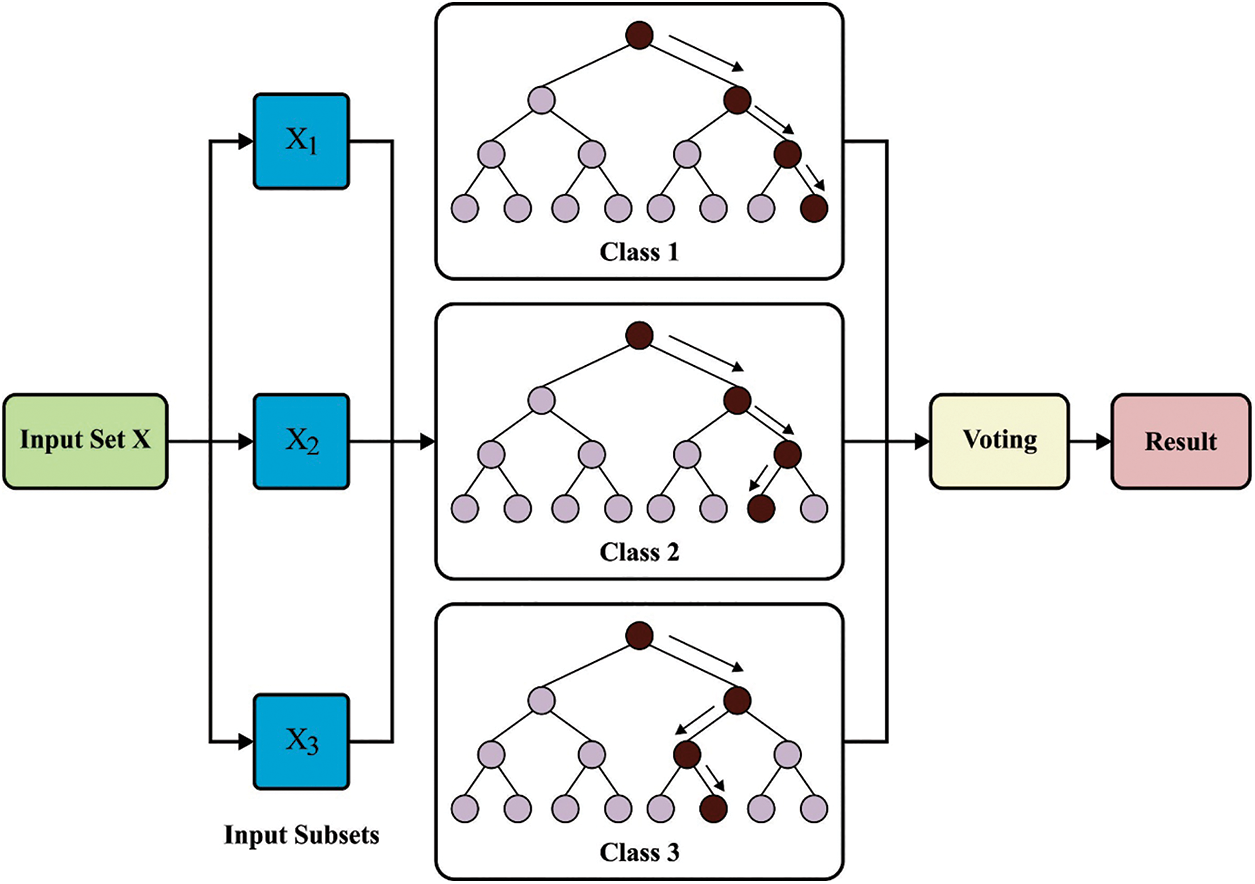
Figure 2: Architecture of RF

3  Experimental Validation

The proposed model is simulated using Python 3.6.5 tool on PC i5-8600k, GeForce 1050Ti 4 GB, 16 GB RAM, 250 GB SSD, and 1 TB HDD. The parameter settings are given as follows: learning rate: 0.01, dropout: 0.5, batch size: 5, epoch count: 50, and activation: ReLU. The performance of the ETSOTL-MIAS model on bone cancer classification performance is tested on a medical dataset comprising 100 samples with two classes as given in Table 1. Fig. 3 illustrates the sample images.

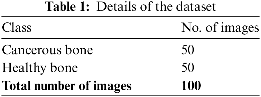
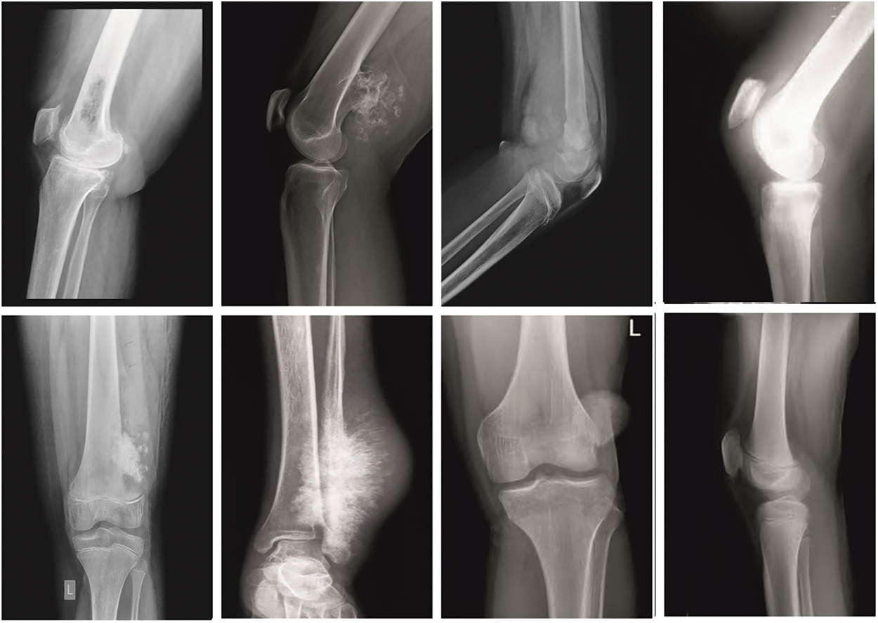
Figure 3: Sample images

The confusion matrices of the ETSOTL-MIAS model are depicted in Fig. 4. On 80% of the TR database, the ETSOTL-MIAS model has identified 37 samples in the cancerous bone and 37 samples in healthy bone. Besides, on 20% of the TS database, the ETSOTL-MIAS technique has identified 10 samples of cancerous bone and 9 samples of healthy bone. In addition, on 70% of the TR database, the ETSOTL-MIAS approach has detected 34 samples of cancerous bone and 28 samples of healthy bone. At last, on 30% of the TS database, the ETSOTL-MIAS approach has identified 12 samples of cancerous bone and 17 samples of healthy bone.

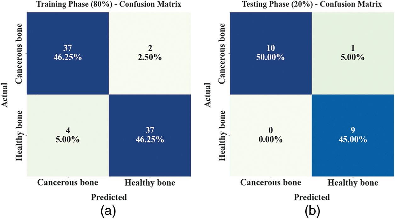
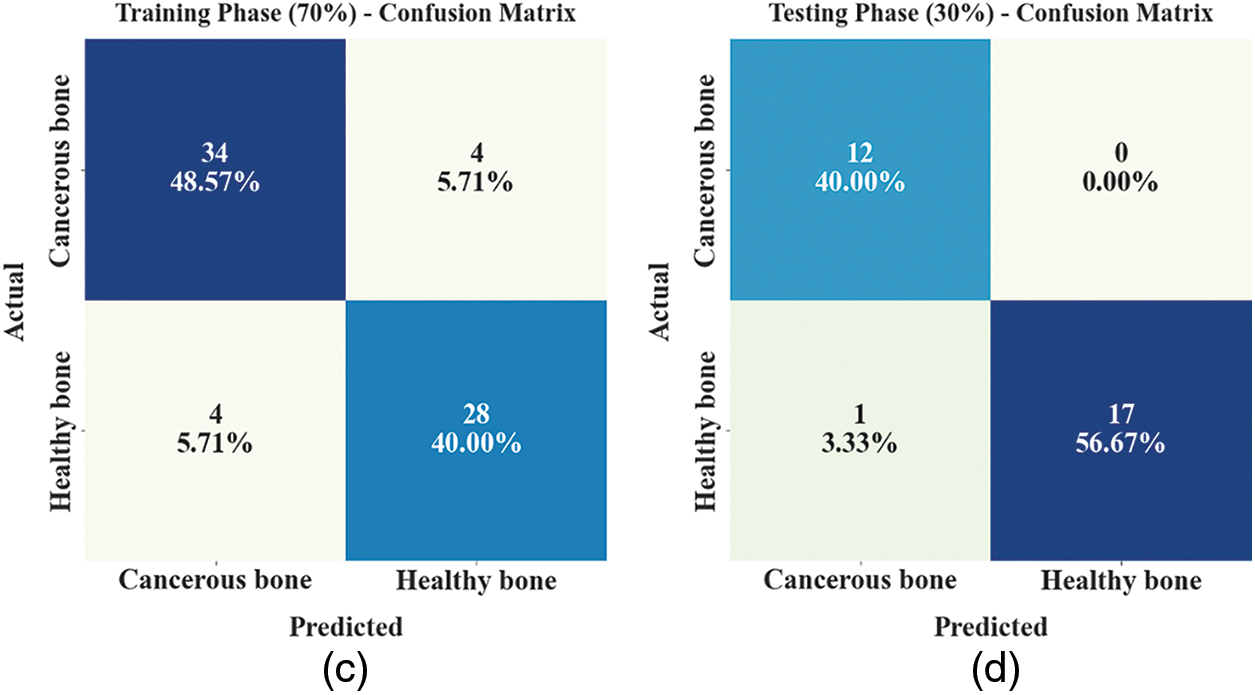
Figure 4: Confusion matrices of ETSOTL-MIAS approach (a)–(b) TR and TS databases of 80:20 and (c)–(d) TR and TS databases of 70:30

An entire classifier result of the ETSOTL-MIAS model with 80:20 of TR/TS data is depicted in Table 2.

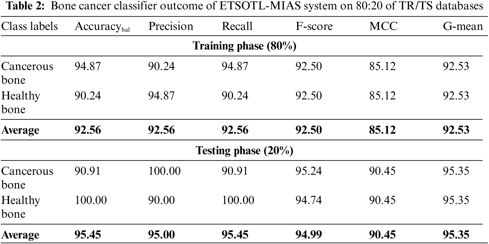
Fig. 5 represents the bone cancer classification outcomes of the ETSOTL-MIAS model with 80% of the TR database. With cancerous bone class, the ETSOTL-MIAS model has reached accubal of 94.87%, precn of 90.24%, recal of 94.87%, Fscore of 92.50%, MCC of 85.12%, and Gmean of 92.53%. Meanwhile, with healthy bone class, the ETSOTL-MIAS method has reached accubal of 90.24%, precn of 94.87%, recal of 90.24%, Fscore of 92.50%, MCC of 85.12%, and Gmean of 92.53%.

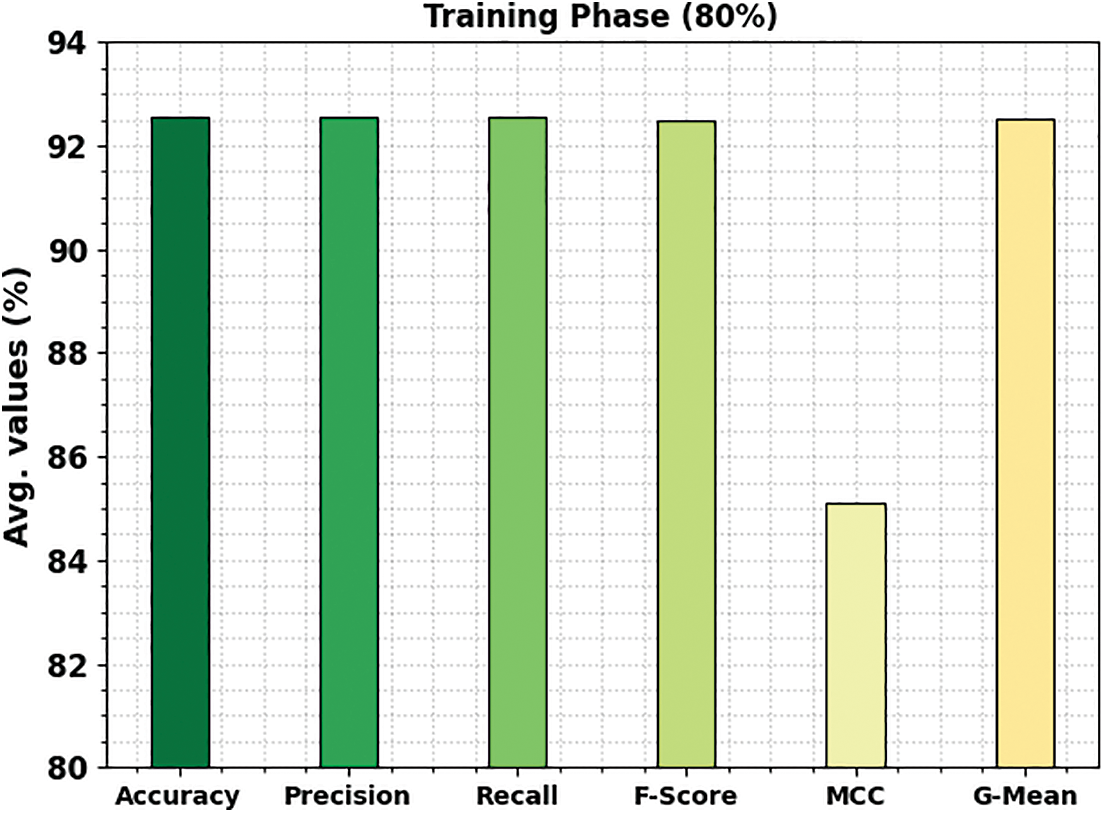
Figure 5: Average outcome of ETSOTL-MIAS system on 80% of TR database

Fig. 6 shows the bone cancer classification outcomes of the ETSOTL-MIAS method with 20% of the TS database. With cancerous bone class, the ETSOTL-MIAS technique has reached accubal of 90.91%, precn of 100%, recal of 90.91%, Fscore of 95.24%, MCC of 90.45%, and Gmean of 95.35%. In the meantime, with healthy bone class, the ETSOTL-MIAS methodology has reached accubal of 100%, precn of 90%, recal of 100%, Fscore of 94.74%, MCC of 90.45%, and Gmean of 95.35%.

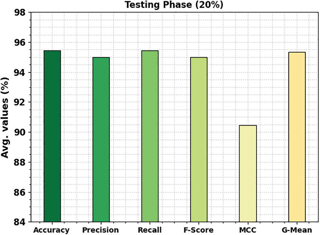
Figure 6: Average outcome of ETSOTL-MIAS system on 20% of TS database

An entire classifier result of the ETSOTL-MIAS model with 70:30 of TR/TS data is depicted in Table 3.

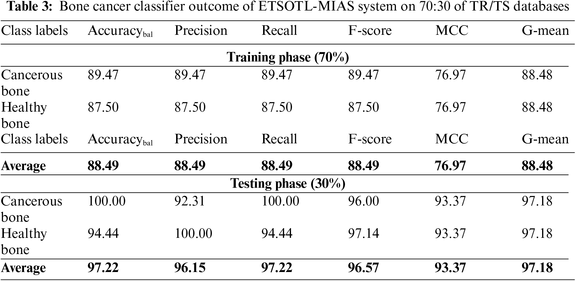
Fig. 7 signifies the bone cancer classification outcomes of the ETSOTL-MIAS technique with 70% of the TR database. With cancerous bone class, the ETSOTL-MIAS approach has reached accubal of 89.47%, precn of 89.47%, recal of 89.47%, Fscore of 89.47%, MCC of 76.97%, and Gmean of 88.48%. In the meantime, with healthy bone class, the ETSOTL-MIAS method has reached accubal of 87.50%, precn of 87.50%, recal of 87.50%, Fscore of 87.50%, MCC of 76.97%, and Gmean of 88.48%.

Figure 7: Average outcome of ETSOTL-MIAS system on 70% of TR database

Fig. 8 shows the bone cancer classification outcomes of the ETSOTL-MIAS method with 30% of the TS database. With cancerous bone class, the ETSOTL-MIAS approach has reached accubal of 100%, precn of 92.31%, recal of 100%, Fscore of 96%, MCC of 93.37%, and Gmean of 97.18%. Eventually, with healthy bone class, the ETSOTL-MIAS methodology has reached accubal of 94.44%, precn of 100%, recal of 94.44%, Fscore of 97.14%, MCC of 93.37%, and Gmean of 97.18%.

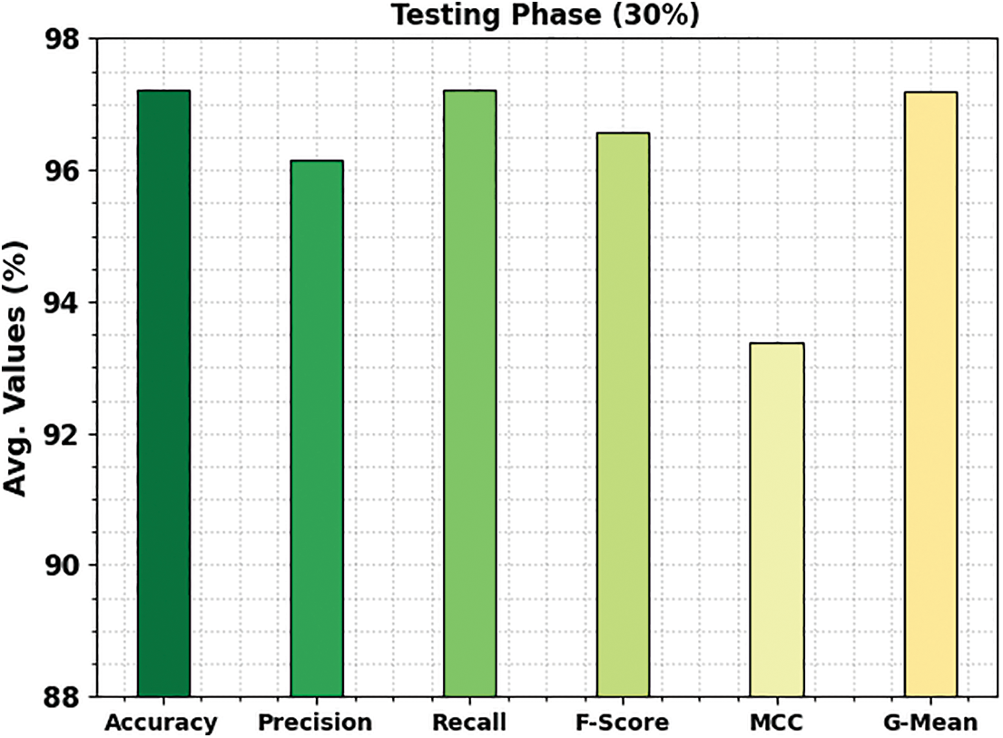
Figure 8: Average outcome of ETSOTL-MIAS system on 30% of TS database

The TACC and VACC of the ETSOTL-MIAS technique are investigated on bone cancer classification performance in Fig. 9. The figure displays that the ETSOTL-MIAS algorithm has shown improved performance with increased values of TACC and VACC. Notably, the ETSOTL-MIAS technique has attained maximum TACC outcomes.

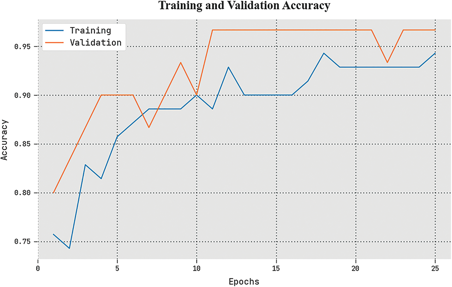
Figure 9: TACC and VACC analysis of the ETSOTL-MIAS system

The TLS and VLS of the ETSOTL-MIAS method are tested on bone cancer classification performance in Fig. 10. The figure exhibited the ETSOTL-MIAS approach has revealed better performance with the least values of TLS and VLS. Seemingly, the ETSOTL-MIAS method has reduced VLS outcomes.

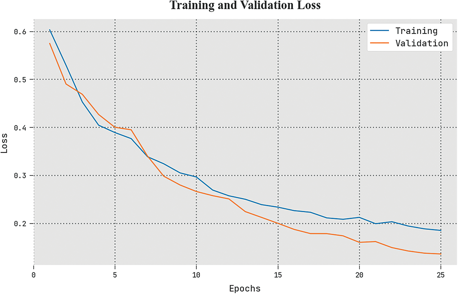
Figure 10: TLS and VLS analysis of the ETSOTL-MIAS system

A clear precision-recall study of the ETSOTL-MIAS algorithm under the test database is given in Fig. 11. The figure shows the ETSOTL-MIAS technique has enhanced values of precision-recall values in several classes.

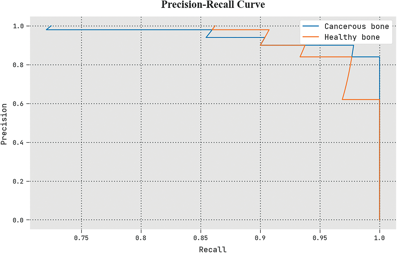
Figure 11: Precision-recall analysis of the ETSOTL-MIAS system

The detailed ROC investigation of the ETSOTL-MIAS technique in the test database is given in Fig. 12. The outcomes exhibited by the ETSOTL-MIAS algorithm have shown its ability in classifying distinct class labels in the test database.

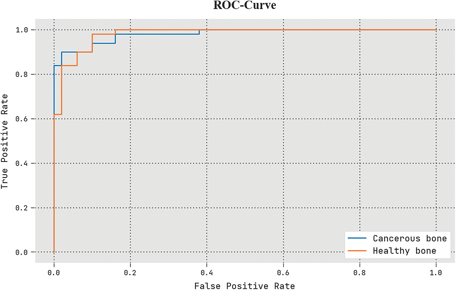
Figure 12: ROC analysis of the ETSOTL-MIAS system

To assuring the improved bone cancer results of the ETSOTL-MIAS model, a widespread comparison study is made in Table 4 [27]. Based on accuy, the ETSOTL-MIAS model has provided a higher accuy of 97.22%. Meanwhile, based on precn, the ETSOTL-MIAS approach has provided a higher precn of 96.15%.

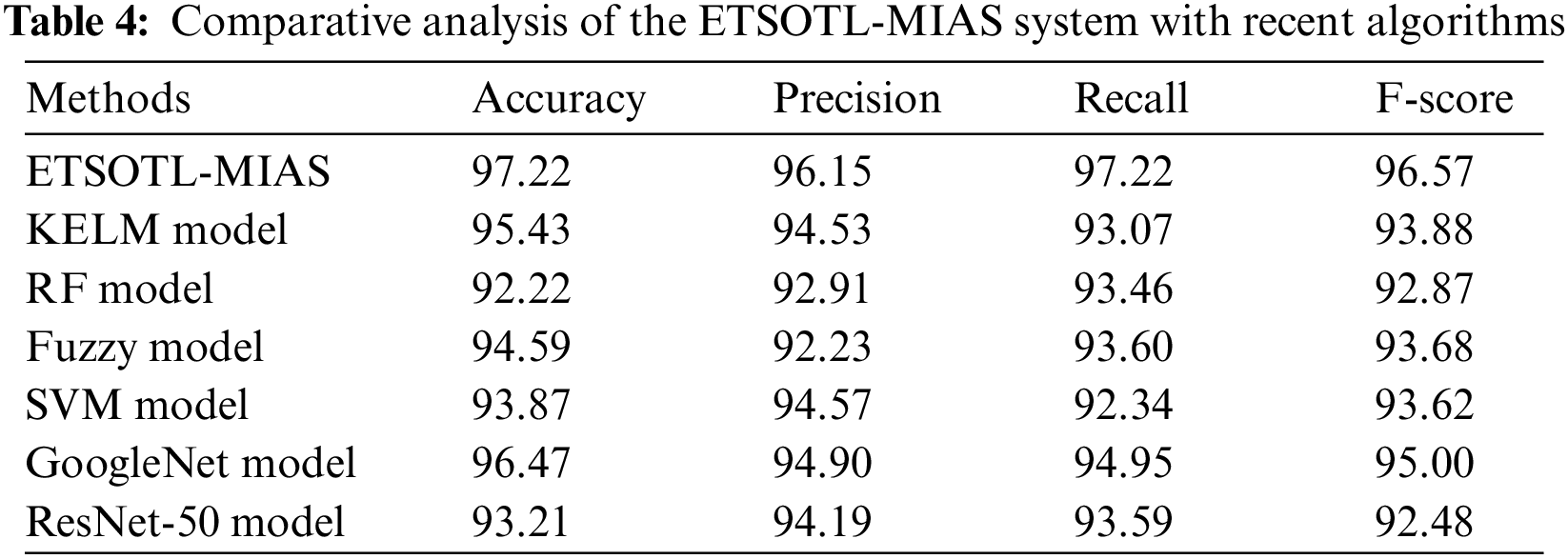
Moreover, based on recal, the ETSOTL-MIAS method has provided a higher recal of 97.22%. Finally, based on Fscore, the ETSOTL-MIAS approach has provided a higher Fscore of 96.57%. These results assured the maximum performance of the ETSOTL-MIAS model on bone cancer identification.

4  Conclusion

In this study, we have developed a new ETSOTL-MIAS technique for the identification and classification of bone cancer on medical imaging. The ETSOTL-MIAS technique involved the design of the Chan Vese segmentation technique to identify the affected regions in the medical image. For feature extraction purposes, the ETSOTL-MIAS technique designs a modified DarkNet-53 model. To avoid the manual hyperparameter adjustment process, the ETSOTL-MIAS technique exploits the ETSO algorithm. Finally, the classification of medical images takes place by the RF classifier. The performance validation of the ETSOTL-MIAS technique is tested on a benchmark medical image database. The extensive experimental analysis showed the promising performance of the ETSOTL-MIAS technique under different measures.

Acknowledgement: The author would like to acknowledge the financial support for this work from the Deanship of Scientific Research (DSR), University of Tabuk, Tabuk, Saudi Arabia.

Funding Statement: The authors would like to acknowledge the financial support for this work from the Deanship of Scientific Research (DSR), University of Tabuk, Tabuk, Saudi Arabia, under grant number S-1440-0262.

Author Contributions: The author confirm contribution to the paper as follows: study conception and design; data collection; analysis and interpretation of results. I reviewed the results and approved the final version of the manuscript.

Availability of Data and Materials: The dataset is collected from different Google images and The TCIA (Cancer Imaging Archive), available at https://imaging.cancer.gov/informatics/cancer_imaging_archive.htm.

Conflicts of Interest: The author declares that they have no conflicts of interest to report regarding the present study.

References

1. M. Sultana, A. Hossain, F. Laila, K. A. Taher and M. N. Islam, “Towards developing a secure medical image sharing system based on zero trust principles and blockchain technology,” BMC Medical Informatics and Decision Making, vol. 20, no. 1, pp. 1–10, 2020. [Google Scholar]

2. S. Namasudra, “A secure cryptosystem using DNA cryptography and DNA steganography for the cloud-based IoT infrastructure,” Computers and Electrical Engineering, vol. 104, pp. 108426, 2022. [Google Scholar]

3. O. Hosam and M. H. Ahmad, “Hybrid design for cloud data security using combination of AES, ECC and LSB steganography,” International Journal of Computational Science and Engineering, vol. 19, no. 2, pp. 153–161, 2019. [Google Scholar]

4. K. C. Nunna and R. Marapareddy, “Secure data transfer through internet using cryptography and image steganography,” in 2020 SoutheastCon, Raleigh, NC, USA, pp. 1–5, 2020. [Google Scholar]

5. L. Kumar, “A secure communication with one time pad encryption and steganography method in cloud,” Turkish Journal of Computer and Mathematics Education, vol. 12, no. 10, pp. 2567–2576, 2021. [Google Scholar]

6. W. A. Awadh, A. S. Hashim and A. Hamoud, “A review of various steganography techniques in cloud computing,” University of Thi-Qar Journal of Science, vol. 7, no. 1, pp. 113–119, 2019. [Google Scholar]

7. M. S. Abbas, S. S. Mahdi and S. A. Hussien, “Security improvement of cloud data using hybrid cryptography and steganography,” in Int. Conf. on Computer Science and Software Engineering, Duhok, Iraq, pp. 123–127, 2020. [Google Scholar]

8. B. Abd-El-Atty, A. M. Iliyasu, H. Alaskar and A. A. Abd El-Latif, “A robust quasi-quantum walks-based steganography protocol for the secure transmission of images on cloud-based E-healthcare platforms,” Sensors, vol. 20, no. 11, pp. 3108, 2020. [Google Scholar] [PubMed]

9. M. O. Rahman, M. K. Hossen, M. G. Morsad and A. Chandra, “An approach for enhancing security of cloud data using cryptography and steganography with e-lsb encoding,” International Journal of Computer Science and Network Security, vol. 18, no. 9, pp. 85–93, 2018. [Google Scholar]

10. S. Arunkumar, S. Vairavasundaram, K. S. Ravichandran and L. Ravi, “RIWT and QR factorization based hybrid robust image steganography using block selection algorithm for IoT devices,” Journal of Intelligent & Fuzzy Systems, vol. 36, no. 5, pp. 4265–4276, 2019. [Google Scholar]

11. R. Adee and H. Mouratidis, “A dynamic four-step data security model for data in cloud computing based on cryptography and steganography,” Sensors, vol. 22, no. 3, pp. 1109, 2022. [Google Scholar] [PubMed]

12. K. B. Madavi and P. V. Karthick, “Enhanced cloud security using cryptography and steganography techniques,” in Int. Conf. on Disruptive Technologies for Multi-Disciplinary Research and Applications, Bengaluru, India, pp. 90–95, 2021. [Google Scholar]

13. A. Sukumar, V. Subramaniyaswamy, V. Vijayakumar and L. Ravi, “A secure multimedia steganography scheme using hybrid transform and support vector machine for cloud-based storage,” Multimedia Tools and Applications, vol. 79, no. 15, pp. 10825–10849, 2020. [Google Scholar]

14. M. A. Khan, “Information security for cloud using image steganography,” Lahore Garrison University Research Journal of Computer Science and Information Technology, vol. 5, no. 1, pp. 9–14, 2021. [Google Scholar]

15. A. A. AB, A. Gupta and S. Ganapathy, “A new security mechanism for secured communications using steganography and cba,” ECTI Transactions on Computer and Information Technology, vol. 16, no. 4, pp. 460–468, 2022. [Google Scholar]

16. L. Gaur, U. Bhatia, N. Z. Jhanjhi, G. Muhammad and M. Masud, “Medical image-based detection of COVID-19 using deep convolution neural networks,” Multimedia Systems, vol. 29, pp. 1729–1738, 2023. https://doi.org/10.1007/s00530-021-00794-6 [Google Scholar] [PubMed] [CrossRef]

17. V. Chouhan, S. K. Singh, A. Khamparia, D. Gupta, P. Tiwari et al., “A novel transfer learning based approach for pneumonia detection in chest X-ray images,” Applied Sciences, vol. 10, no. 2, pp. 559, 2020. [Google Scholar]

18. V. Arora, E. Y. K. Ng, R. S. Leekha, M. Darshan and A. Singh, “Transfer learning-based approach for detecting COVID-19 ailment in lung CT scan,” Computers in Biology and Medicine, vol. 135, pp. 104575, 2021. [Google Scholar] [PubMed]

19. M. S. Ali, M. S. Miah, J. Haque, M. M. Rahman and M. K. Islam, “An enhanced technique of skin cancer classification using deep convolutional neural network with transfer learning models,” Machine Learning with Applications, vol. 5, pp. 100036, 2021. [Google Scholar]

20. M. S. Al-Rakhami, M. M. Islam, M. Z. Islam, A. Asraf, A. H. Sodhro et al., “Diagnosis of COVID-19 from X-rays using combined CNN-RNN architecture with transfer learning,” medRxiv, 2021. https://doi.org/10.1101/2020.08.24.20181339 [Google Scholar] [CrossRef]

21. I. D. Apostolopoulos and T. A. Mpesiana, “COVID-19: Automatic detection from X-ray images utilizing transfer learning with convolutional neural networks,” Physical and Engineering Sciences in Medicine, vol. 43, no. 2, pp. 635–640, 2020. [Google Scholar] [PubMed]

22. D. N. Thanh, N. N. Hien, V. B. S. Prasath, L. T. Thanh and N. H. Hai, “Automatic initial boundary generation methods based on edge detectors for the level set function of the Chan-Vese segmentation model and applications in biomedical image processing,” in Frontiers in Intelligent Computing: Theory and Applications, Advances in Intelligent Systems and Computing Book Series, vol. 1014. Singapore: Springer, pp. 171–181, 2019. [Google Scholar]

23. K. Jabeen, M. A. Khan, M. Alhaisoni, U. Tariq, Y. D. Zhang et al., “Breast cancer classification from ultrasound images using probability-based optimal deep learning feature fusion,” Sensors, vol. 22, no. 3, pp. 807, 2022. [Google Scholar] [PubMed]

24. M. Tubishat, M. A. Abushariah, N. Idris and I. Aljarah, “Improved whale optimization algorithm for feature selection in arabic sentiment analysis,” Applied Intelligence, vol. 49, no. 5, pp. 1688–1707, 2019. [Google Scholar]

25. S. I. Shyla and S. S. Sujatha, “Cloud security: LKM and optimal fuzzy system for intrusion detection in cloud environment,” Journal of Intelligent Systems, vol. 29, no. 1, pp. 1626–1642, 2020. [Google Scholar]

26. A. Palczewska, J. Palczewski, R. ese Robinson and D. Neagu, “Interpreting random forest classification models using a feature contribution method,” in Integration of Reusable Systems, Advances in Intelligent Systems and Computing Book Series, vol. 263. Cham: Springer, pp. 193–218, 2014. [Google Scholar]

27. A. Sharma, D. P. Yadav, H. Garg, M. Kumar, B. Sharma et al., “Bone cancer detection using feature extraction based machine learning model,” Computational and Mathematical Methods in Medicine, vol. 2021, pp. 1–13, 2021. [Google Scholar]