An Artificial Intelligence-Based Framework for Fruits Disease Recognition Using Deep Learning

1  Introduction

Feeding the fast-growing population is becoming a major challenge, especially when the climate conditions are changing and affecting the agriculture sector by introducing various risks in the form of different crop/fruit diseases [1]. Even though the production of fruit quantity and quality is enhanced due to technological advancements, 14.3% of people still suffer from malnutrition [2]. Additionally, due to population growth, there is a daily decrease in land available for cultivation. As a result, it is imperative to cultivate a healthy and sufficient quantity of crops or fruit to meet the needs of the people [3]. Fruits are necessary for humans because they provide several critical nutrients, such as vitamins C and A, folate, potassium, and dietary fiber [4]. However, fruit diseases are causing great losses in the revenue of important fruit crops every year [5]. Early detection and precise disease classification are essential for reducing the consequences of fruit diseases. Identifying a variety of fruit illnesses is crucial because farmers want to experiment with crops besides local plants on their farms, which is only feasible if an automated disease detection system supports both competent and inexperienced farmers [6].

While each location has distinctive regional fruit harvests consumed daily, some fruits, including apples, grapes, and citrus, are grown worldwide [7]. The research’s target plants are the fruit above crops because of their high production and consumption rates. Manual disease identification takes a lot of time and resources, including people, knowledge of fruit crops, and agricultural equipment [8]. Furthermore, it is impossible to accurately carry out the classification work in the real-time environment or the field areas due to the complexity of disease symptoms and the similarity of different diseases [9]. Visualizing people and identifying infections through microscopic research are two methods that could be used for manual disease detection. It also covers methods like molecular and microbiological diagnostics [10]. These meticulous manual and conventional procedures take time and demand more human labor and knowledge. The data shows that agricultural diseases are significant in the expanding population’s food shortage. The prospects of increased crop output are increasing daily thanks to developments in computer vision, AI methods, and sensor-based technologies [11]. This data collected through sensors or satellite imagery is fused to make better models for predicting the crop’s life cycle, including diseases and remedies [12]. Automated computer-based programs support decision-making, disease classification and prediction, fruit and vegetable quality classification, and soil quality classification. The application of imaging techniques, such as picture acquisition and subsequent image processing, is included in the computer science field of computer vision [13]. Some common computer-based techniques used for plant disease detection are classical techniques, preprocessing, segmentation, feature extraction, and classification methods.

The images taken in a real-world situation have a lot of noise and different illumination intensities. Therefore, disease classification suffers if the classifier directly supplies the actual image [14]. Several preprocessing processes are carried out to enhance the visual representation of samples to address these problems. Image segmentation is one such method. The Region of Interest (ROI) was correctly identified due to the segmentation procedure, which attempted to remove the unhealthy portion of the plant leaf. To perform recognition, it then uses it as input. To extract information and recognize objects or diseases, segmentation in computer vision entails dividing the existing image into segments or portions [15]. The segmentation technique also makes it easier to recall aberrant regions by reducing the complexity of the space and the input image data. The image’s boundaries and the necessary ROI are obtained as part of this procedure. Different techniques, such as K-means clustering [16], Otsu’s threshold algorithm [17], or by using boundary detection algorithms [18], can be used to segment data.

The feature is the basic information that helps solve computational issues in computer vision and machine learning [19]. For instance, a feature might be the edge or contour of an image. Multiple feature extraction techniques must be used on a sample since, typically, just one or two types of features are sufficient to extract the needed information. For instance, it takes a lot of time and requires more human resources to detect and identify plant diseases manually. Therefore, it is necessary to install an automated system on large-scale fields [20]. Deep learning-based models may be applied to many crops and have good classification accuracy. Farmers already utilize deep learning models for precise classification, which aids in producing high-quality crops and improves the quality. Thanks to advances in deep learning, there is no longer a requirement to separately apply feature extraction for categorization. It is possible to complete both procedures in a single unit [21]. A subset of machine learning (ML) and artificial intelligence (AI) called “deep learning” seeks to mimic the functions of the human brain in areas including speech recognition, object detection, and decision-making. In the past few years, deep learning has shown encouraging results in detecting and recognizing illnesses in agriculture. While deep learning techniques are more beneficial for large-scale datasets, classical machine learning techniques have been used successfully in agriculture when there is a limited amount of data. Convolutional layers are used in deep learning to extract an image’s more detailed information. The key driver of deep learning in agriculture is feature learning across multiple layers of hierarchies. The complicated model design allows the DL features to handle the challenging imaging situation more effectively [22,23].

Scientists have reported huge work for the timely and accurate identification and classification of fruit diseases; however, here are some major challenges which degrade the system accuracies: (i) Similar characteristics of crop symptoms, such as their color and texture, make confusion for correct recognition into their relevant class, (ii) Change of symptoms shapes for disease regions and (iii) Variations in illumination and background are the major challenges for accurate recognition. In addition, the presence of irrelevant and redundant information reduces recognition accuracy. This work focuses on overcoming the mentioned problems by presenting an ensembling technique involving four primary stages: contrast improvement, feature computation, feature fusion & selection, and classification. Our work employs a multi-layer feature fusion and best feature selection approach. The main contributions of the proposed work are as follows:

i)    Prepare a hybrid dataset containing both original and noisy data for learning fine-tuned deep learning models.

ii)   A pre-trained deep model efficient net-b0 is employed and fine-tuned in terms of layer addition and layer removal. After that, deep transfer learning trained the model on original and noisy data and extracted deep features.

iii)   Deep features of the noisy and original dataset have been fused using a new serially controlled descending-order probability approach.

iv)   A path-find optimization technique is chosen and improved by employing the higher probability value. The best features are employed for the final classification.

v)   An extensive experiment analysis is performed compared to the latest approaches to show the robustness of the proposed framework.

The later sections of the paper are organized as follows: the existing work on this topic is mentioned in Section 2. Then, the presented technique is given in Section 3, while the experimental evaluations are described in Section 4. Finally, in Section 5, the conclusion and plan of the proposed work are elaborated.

2  Related Work

Many researchers are working in the field of computer vision and machine learning to enhance the process of fruit disease detection and classification. Bansal et al. [24] discussed the importance of automated disease detection and classification in fruit plants because the manual process is tedious and time-consuming. A country’s economy, especially agriculture, depends on good quality and quantity of food, which highly depends on early disease detection. In the proposed model [24], a concatenation of features computed from DenseNet and EfficientNet-B7 is performed to classify apple leaf diseases. The publically available apple leaves dataset is used [25]. The dataset contains four data classes: healthy, apple scab, apple rust, and other diseases, including brown and yellow leaf spots. Data augmentation is performed to minimize the problem of overfitting [26]. Data augmentation includes flipping, noise addition, rotation, and shifting in data. Canny Edge Detection [27] is used for edge detection, which helps reduce Area of Interest (AoI).

Multiclass classification is performed because the dataset includes more than two classes for classification. The proposed model gives an accuracy rate of 96.25%. Li et al. [28] proposed that intelligent and early disease detection and classification play a vital role in enhancing the quality and quantity of fruit crops. The respective research presents a CNN-based model RegNet, which deals with five classes of apple leaf datasets. For validation, the proposed model is compared with other state-of-the-art models, namely EfficientNet-B0, MobileNet-V3, and ShuffleNet; for data balancing, multiple data enhancement techniques are used: image rotation, translation, scaling, and brightness calibration. In training a CNN model, the learning rate is an important parameter. It is a range of hyper-parameters that are updated in each iteration. A good learning rate adjustment can enhance the convergence speed of any model. Adam Optimizer is used in the respective research work, which enhanced the selection process of suitable learning rate. An accuracy rate of 99.23% is attained with the help of the proposed RegNet model and Adam Optimizer. Di et al. [29] presented that several researchers are using deep learning methods to detect fruit disease at its early stages.

Due to the difficulty of identifying numerous illnesses, a new model called DF-Tiny-Yolo is suggested for apple leaf disease detection. For evaluation, the suggested model is tested on four different data classes. The DenseNet model, which aids in feature propagation, increases detection accuracy. The proposed model achieved a 90.88% average Intersection over Union (IoU) and 99.2% Mean Average Precision (MAP). The introduction of DenseNet significantly reduces the vanishing gradient issue during model training.

Additionally, the feature of DenseNet helps connect the many model layers by creating connections between them, allowing for the reuse of features and assisting in reducing the overfitting issue. The performance measures in [29] are precision, recall rate, and average IoU. Gu et al. [30] proposed a model based on improved deep learning methods and K-Nearest Neighbor (KNN).

Apples and pears are the fruit trees that are being considered. Six distinct data classes—fire blight, Alternaria leaf spot, anthracnose, scab, marssonina blotch, and black necrotic—have been approved for testing. Seven pre-trained models—VGG-16, VGG-19, Inception ResNet, ResNet-50, DenseNet-121, EfficientNet-B0, and NasNet—extract deep features. The RoI is manually trimmed from the photos, improving recognition precision. The pre-trained CNN models are then fed the retrieved images for final optimization. The KNN algorithm is then used to detect related symptoms using the extracted features. The performance of each research is measured by its precision and accuracy, with ResNet-50 achieving the greatest precision rate of 98.83%. Syed-Ab-Rahman et al. [31] discussed the effects of fruit disease on crop yield, reducing the economy of any agricultural country. According to research, Citrus is an important fruit crop cultivated on a large scale; hence, attacks of pests and other diseases cause significant losses in its production. In the respective research work, a two-stage model is presented, which is based on Deep Convolutional Neural Network (DCNN). In the first stage region-based network model is proposed, and in the second stage, a suitable classifier is used to classify the potential region-based disease. The proposed model yields an accuracy rate of 94.37%, obtained on classes of three diseases: bacterial canker, huanglongbing, and black spot. In the pre-processing of available data, multiple steps are taken, i.e., they are initially converted into a greyscale, then histogram equalization is applied to stabilize the range of intensities. Finally, a Faster R-CNN model is applied, a four-stage network model including feature extraction, Region Proposal Network (RPN), pooling, i.e., Region of Interest (RoI), and classification.

The authors of the methodologies above performed classification after using pre-trained models for training. A few writers created customized models and extracted characteristics that were subsequently categorized using machine learning classifiers. The studies mentioned above did not use noisy data for training. The scalability of a model can be improved by training it on noisy data. Additionally, they did not concentrate on feature optimization to shorten the computational time.

3  Proposed Work

This section explains the proposed methodology as shown in Fig. 1. First, the dataset of three fruit leaf diseases, including apple, Citrus, and grapes leaves, is collected for evaluation. The originally obtained samples are given the name original data, whereas the data in which different artifacts are added is called noisy data. Then, on both the original and noisy data, a finely tuned EfficientNet-B0 Deep Convolutional Neural Network model is applied using transfer learning. As a result, two newly trained models, namely Model 1 and Model 2, are obtained. Then, the state-of-the-art feature extraction technique is applied to obtain useful and non-redundant features, which are later fused to get original and noisy data features. Finally, the path Finder Algorithm (PFA) based optimization technique is applied to obtain a set of optimized features classified using multiple classifiers, including Medium Neural Network, Wide Neural Network, Support Vector Machine, and others for classification.

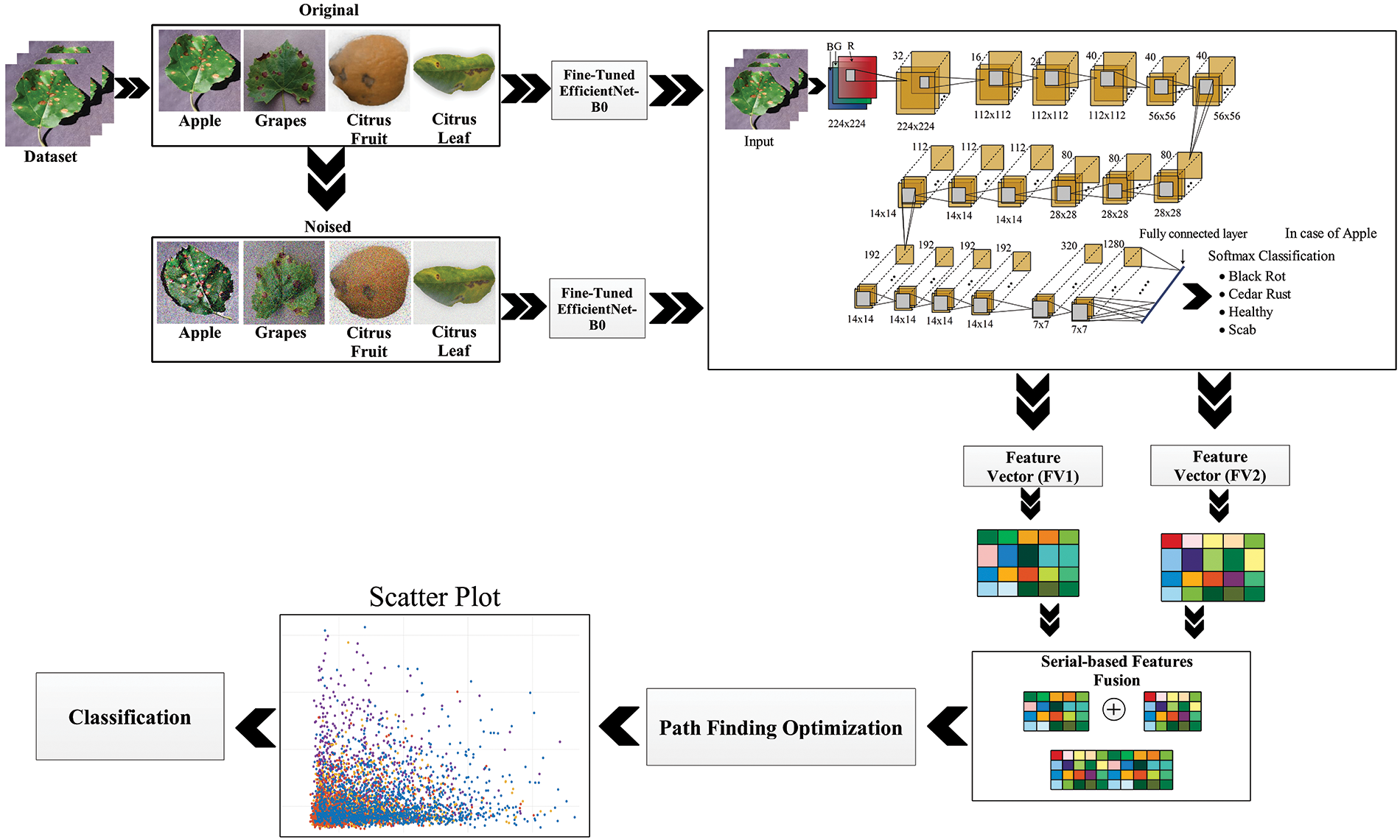
Figure 1: Proposed deep learning and optimization-based framework of fruit disease classification

3.1 Database Preparation

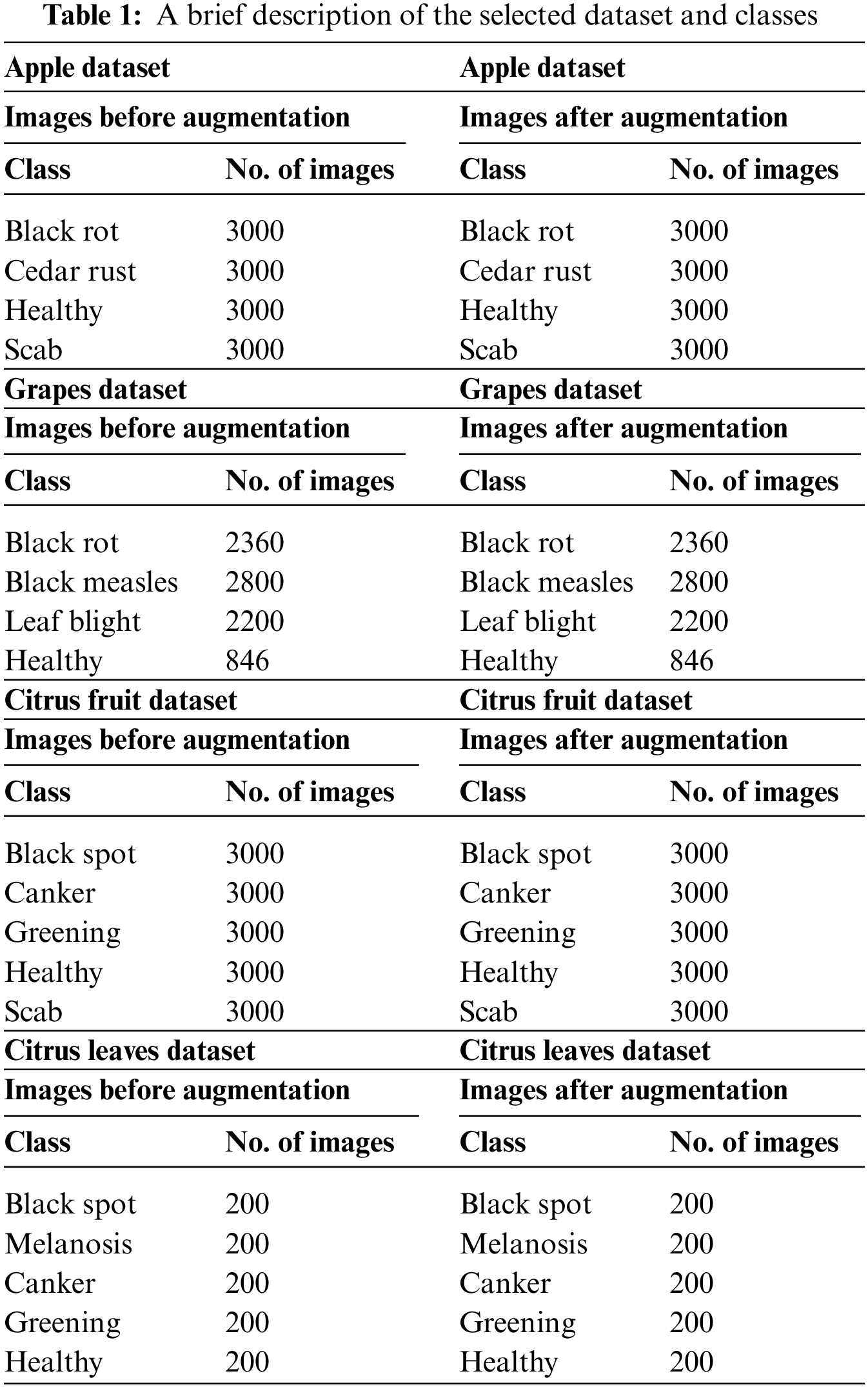
The database created for the evaluation is divided into two parts: the original dataset and the noisy dataset. The original dataset is comprised of three fruit leaves, including apples, grapes, and Citrus. Apple dataset contains four classes of data, including three classes of diseased leaves and one class of healthy leaves. The other three classes involve black rot, cedar rust, and scab. All four classes contain an equal number of images, i.e., 3000 of each class. The grapes dataset contains data of four classes, including healthy with 846 images, black rot with 2360 images, esca (black measles) with 2800 images, and leaf blight with 2200 images. Citrus is divided into citrus fruit and Citrus leaves data. The Citrus fruit dataset contains five classes: healthy, canker, black spot, greening, and scab. Each class contains an equal number of images, i.e., 3000 images in each class. The Citrus leaves dataset contains five classes with approximately 200 images of each class; classes include black spot, canker, greening, healthy, and melanosis. The images of the original dataset are shown in Fig. 2. For training and testing of the proposed architecture, 50:50 of the available datasets have opted to validate our results.

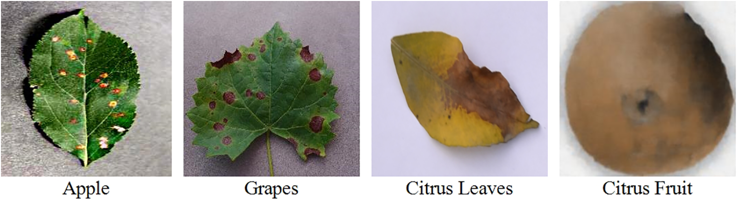
Figure 2: Sample images of the original dataset

The noisy database contains the same fruit leave diseases as used for the original data but with an additional noise added to the available dataset. Apple, Citrus, and grapes fruit leaves are used for evaluation purposes with the same number of images as used for the original. The type of noises added to the data are Gaussian Noise, Uniform Noise, Rayleigh Noise, Exponential Noise, and Salt and Pepper Noise. A few samples from the noisy dataset are given in Fig. 3. The detail of each class’s images is also given below in Table 1.

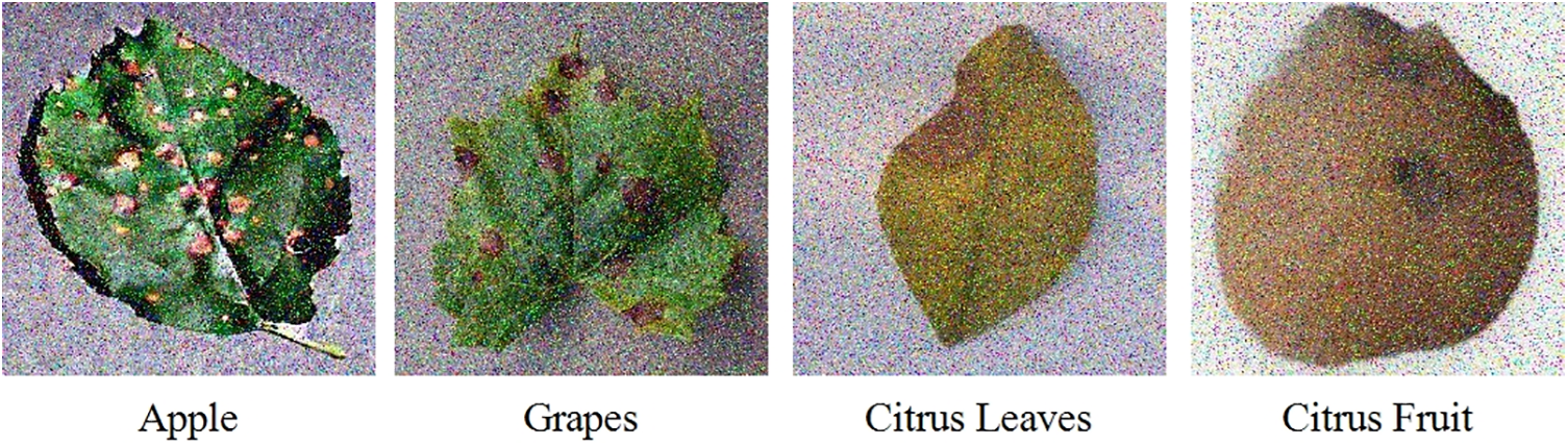
Figure 3: Sample images of the noisy dataset

3.2 Convolutional Neural Network

Before the advent of CNN models, the recognition or classification process involved extracting features that were either insufficient or did not achieve a higher level of accuracy [32]. CNN models are achieving higher levels of accuracy efficiently in all fields in which it is deployed. CNN models also follow a set of algorithms involving backpropagation, including convolutional and pooling layers and steps like feature extraction. The working of Neural Networks is based on mimicry of the human brain to the possible level. CNN involves multiple convolutional layers and helps recognize digital images or data.

The convolutional Layer is the most important and basic in a CNN architecture [33]. In this layer, the respective image’s activation function or map is generated by convolving the matrix of image pixels. The activation map is useful in storing the values of discriminant features, hence reducing the amount of data for processing. Convolution is the most important step of any CNN model, and Convolutional Layer (CL) is the most important layer among other layers. It is responsible for the 2D convolution of input and kernel in the forward go. In the beginning, the weights of kernels are selected randomly and then updated as the iteration moves on. The loss function updates weights as the network training starts. Ultimately, the final learned kernel can detect some patterns in the input image. The three steps of CL involve convolution initially, then stack and Non-Linear Activation Function (NLAF) at the end. Mathematically, let Y be the input matrix, and X. denotes its output. Let’s suppose a set of kernels such that. Hk,∀kϵ[1,…,k], output O(k) convolution after step 1 of convolution is given by [34]:

Ok=Y∗Hk,∀kϵ[1,…,k](1)

where * shows the operation of convolution. It is the dot product between inputs and the filter. In the second step of the stack, all the activation maps Ok are combined to form a new activation map which is 3D in nature, as mentioned in Eq. (2):

B=J(O1,…,Ok)(2)

where K is the total number of filters and J shows the compilation operation of activation maps. Three matrixes input, filter, and output sizes J are assumed such that:

J={ZI×SI×TIZm×Sm×TmZc×Sc×Tcy=Y y=Hk, kϵ[1,…,k]y=0(3)

where Z, S, and T are the height, width, and number of channels, respectively. I, m, and c in the subscript denote the input, filter, and output. There are two equalities first one is TI=Tm, i.e., channels of input are equal to the number of channels of filters. Secondly, Tc=k, i.e., the number of output channels equals the number of filters k. The values of Zc,Sc and Tc can be interpreted after a supposition such that D be the padding and F be the stride, as elaborated in Eqs. (4) and (5):

Zc=1+gfl[(2×D+ZI−Zm)/F](4)

Sc=1+gfl[(2×D+SI−Sm)/F](5)

where gfl is the floor function, the NLAF uses rectified Linear Unit (ReLU) function [35]:

σReLU=ReLU(bik)=max(0,bik)(6)

where bikϵB, members of the activation map B. ReLU is used extensively due to its better performance than other functions, such as the sigmoid function and hyperbolic tangent functions. Better gradient propagation is also one of the reasons for the ReLU function’s good performance.

Pooling Layer: The important function of this layer is to reduce the spatial dimensions of a given feature map without losing key information from the map. As a result, the number of features to be learned by the training model is reduced, and the problem of overfitting is resolved through pooling [36]. The pooling layer helps the CNN model learn all the dimensions of an input image, making the recognition process efficient. There are different types of pooling layers, like max and average pooling layers. Pooling, also called down-sampling, is an operation performed in a local region. It saves the information that is either redundant or unique in the neighbor of receptive fields and gives dominant information as an output response from that local region, as given in Eq. (7):

Xnm=hp(Znm)(7)

where, Xnm shows the pooled feature map of nth layer, for mth input feature map given by Znm and hp is given as the type of pooling operation performed.

Fully Connected Layer: The last layer fed to the neural network is a fully connected layer used for classification. A fully connected layer’s operation differs from convoluting and pooling layers because it is a globally performed operation [37]. This layer can also replace the global average pooling layer [38]. It takes features as input and then analyses the output globally of the previous layers. To mathematically define an FC layer, assume h and l as input and output dimensions, respectively. Weight Matrix G∈Hh,l(R) where h is rows and k are columns. The bias vector is given by a∈Rh, the input vector is given by g∈Rk and activation function is given by z.

FC(g)=z(Gg+a)∈Rh(8)

3.3 Pre-Trained Deep Model: EfficientNet-B0

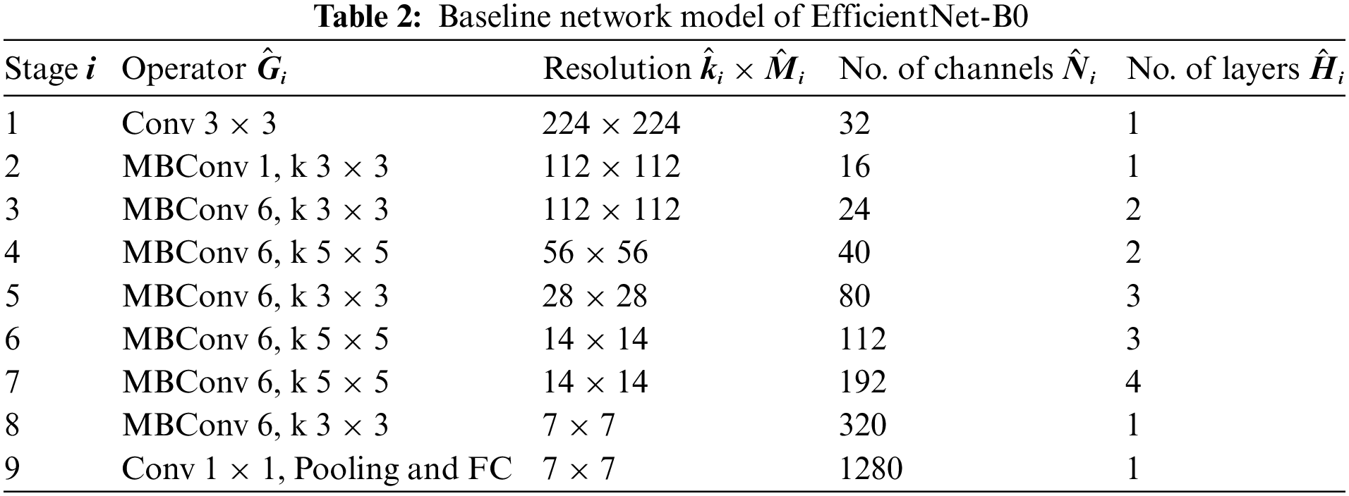
EfficientNet-B0 is trained on more than one million images of the ImageNet dataset [39]. It is a CNN model that can classify the images into 1000 classes of objects. The input size of images for this model is 224-by-224 and contains 290 × 1 CNN layers [40]. Scaling a model does not change the operator. G^i of the layer in the baseline network model. Due to resource constraints, there is a need for model scaling in the convolutional network, which is possible through different methods. For example, ResNet-18 and up models [41] adjust network depth, i.e., the number of network layers. Wide-ResNet [42] controls the width of a network, i.e., the number of network channels. In EfficientNet, three-way model scaling is performed by depth, width, and resolution. Targeted accuracy is maximized by keeping in view the three constraint resources, i.e., depth d, width w, and resolution r, which are given by the equations given below:

maxd,w,rAccuracy(C(d,w,r))(9)

where C stands for convolutional network and is defined as:

C(d,w,r)=Θi=1,…,8G^id.H^i(Y<r.k^i,r,M^i,w.N^i>)(10)

A baseline network model is developed, which helps optimize accuracy and FLOPS (Floating point operations per second). The architecture of EfficientNet-B0 is depicted in Table 2.

3.4 Transfer Learning

Transfer learning is mathematically defined as follows for fruit leaf disease classification [43]. A domain H is considered, which is divided into two parts, i.e., a feature vector space Y and a probability distribution function given by P(Y), Y = [y1, …, yn] ∈ Y. yi is the ith feature vector or instance, n is the total number of features in Y, and Y is the possible space of feature vectors. A task L of a given domain H is divided into two parts one is predictive function h(.), and the other is labeled space J; these two are learned from feature vectors of labeled pairs [yi, ji] where yi∈ Y, ji∈ J. Labels are denoted by J, which contain the values true and false, function h(y) denotes the learner which predicts the value of labels. From this explanation, domain H and task L are given by H = [Y, P(Y)] and L = [J, h(.)]. Now consider data of the source domain as Hs = [(ys1, Js1), …, (ysn, Jsn)], here ysi ∈ Ys which is the ith instance of source data Hs and Jsi∈ Js is the class label for corresponding Ysi. Similarly, target domain HT is given by HT = [(yT1, JT1), …, (yTn, JTn)] where yTi ∈ YT represents the ith instance of target data HT also JTi ∈ J is the respective class label for yTi. The predictive function is given by hs(.), and the predictive function is given by hT(.). By the above-given variable, transfer learning is defined as a process to improve the predictive function of target data hT(.) by using the source domain Hs and source task Ks, where Hs ≠ HT. A graphic view of the transfer learning is shown in Fig. 4.

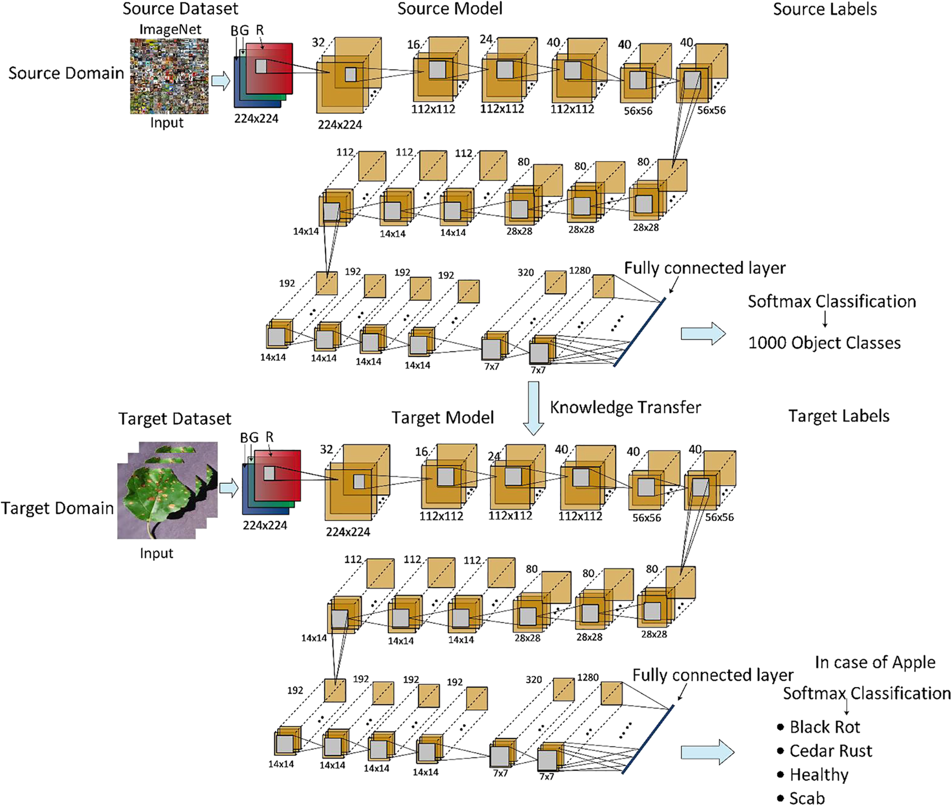
Figure 4: Transfer learning process representation for fruit leaf disease classification

In the fine-tuning process, the last three layers of EfficientNet-b0 models have been removed and added three new layers have fully connected, softmax, and classification output. After that, trained the model separate from the original images and generate noisy images. Several hyperparameters have been initialized randomly, such as a learning rate of 0.0003, epochs of 50, momentum value of 0.625, and SGD optimizer. Then training was performed using the transfer learning concept, and two new models were obtained for the feature extraction process.

3.5 Novelty 1: Features Extraction and Fusion

After the training using TL, features are extracted from the average pooling layer and obtained two feature vectors of dimension N×1280 and N×1280, respectively. Feature fusion is performed later using the serial concatenation probability approach. Fusion is a process in which more than one feature vector is combined to get one feature vector, which is more appealing and discriminative than the input feature vectors.

Let us have two feature vectors, h1(i) and h2(i) having dimensions N × 1280 and N × 1280, respectively. Suppose a fused vector of dimensions (N × 1280 + N × 1280) represented by h3(i). The proposed fusion approach is based on the following three steps.

In the first step, the probability of each feature value is computed and sorted features into descending order. Mathematically, it is represented from Eqs. (11)–(14), respectively.

Pi(h1)=∑i=1h⁡h1(i)N(11)

Pi(h2)=∑i=1h⁡h2(i)N(12)

d(h1)=Descending(Pi(h1))(13)

d(h2)=Descending(Pi(h2))(14)

where Pi(h1) denotes the probability values of feature vectors h1, Pi(h1) denotes the probability values of feature vectors h2, d(h1) denotes the descending value of h1, d(h2) denotes the descending value of h2. In the next step, both vectors d(h1) and d(h2) are fused in one matrix as:

Fusion=(d(h1)d(h2))(N×k1+N×k2)(15)

where k1 and k2 are 1280, and the total features after the fusion process are 2560.

3.6 Novelty 2: Improved Path Finder Algorithm (PFA) Optimization

Path Finder Algorithm (PFA) is a metaheuristic optimization algorithm [44]. This algorithm is also like other swarm-based intelligence algorithms. This algorithm is derived from the rules of living beings for their survival. Besides swarm-based intelligence algorithms, one plus point in PFA is that it is limited to only one species. If this algorithm take the example of the grey wolf algorithm, it is based on only the population of grey wolves. In PFA, the algorithm is based on the animal group, which is divided into two types depending on the fitness value. Two types of classes are the leader and followers, where the leader has a small fitness value. The leader is responsible for finding the path and location of food or hunt and leaving traces for the followers to reach the destination. The followers follow Pathfinder based on traces left by the leader. There is uncertainty for both the Pathfinder and the follower. The role of Pathfinder and follower become interchangeable after running some iterations by the algorithm based on searching capabilities, i.e., the Pathfinder can become a follower and vice versa (Pseudocode 1). For problem optimization, PFA is divided into two phases. Exploration is the first phase in which the location is updated by the PFA using the following updating formula:

abm+1=abm+2h3.(abm−abm−1)+Z(16)

where abm+1 reflects the updated position vector of Pathfinder, abm is the current position vector of Pathfinder, abm−1 is representing the previous position vector of Pathfinder, Z is generated in each iteration given below, random vector h3 is uniformly generated in the range [0,1], m is the number of current iterations. Exploitation is the second phase of PFA in which location updating is performed; updating of location is given below:

ajm+1=ajm+X1.(alm−ajm)+X2.(abm−ajm)+∈,j≥2(17)

∈=(1−mmmax).v1.Yjl,Yjl=‖aj−al‖(18)

Z=v2.e−2mmmax(19)

where v1 and v2 are randomly generated vectors that lie in the range of [−1,1], Yjl represents the distance between two members of the swarm or herd, m is the current iteration number and mmax are the maximum number of iterations. For guaranteed random and multidimensional motion, ∈ and Z must lie in an appropriate range. The fine-KNN classifier is employed as a fitness function in this work and obtained a selected feature vector of dimension N×722. The selected features are sorted into descending order and computed as a probability value. A threshold function is developed based on the highest probability value and selects only the features under that value.

4  Results and Discussion

Experimental Setup-The findings that were reached for the three different fruit plants—apples, grapes, and citrus—are covered in this section. To clarify the effectiveness of the proposed study, first discussed the results for each fruit separately before comparing them with more recent methods. The suggested framework is assessed using 10-fold cross-validation and a 50:50 evaluation ratio. Several hyperparameters have been initialized for fine-tuning deep learning models, including a learning rate of 0.0003, epochs of 50, momentum value of 0.625, and SGD optimizer. Several classifiers have been used for classification accuracy, and each classifier’s performance is evaluated using accuracy and time measures.

4.1 Apple Dataset Results

Accuracy and training time is the main statistical measures to evaluate the proposed methodology. For experimentation, four classes of apple data are used, namely black rot, cedar rust, scab, and healthy, which are evaluated by using 10-fold cross-validations. In the case of the apple plant, the highest classification accuracy rate of 100% is achieved on Medium Neural Network (M-NN) classifier with a training time of 14.303 s. This accuracy is achieved after implementing an optimizer, i.e., Path Finder Algorithm (PFA) based optimization technique. Cubic Support Vector Machine (C-SVM) and Wide Neural Network (W-NN) classifiers also gave good accuracy rates.

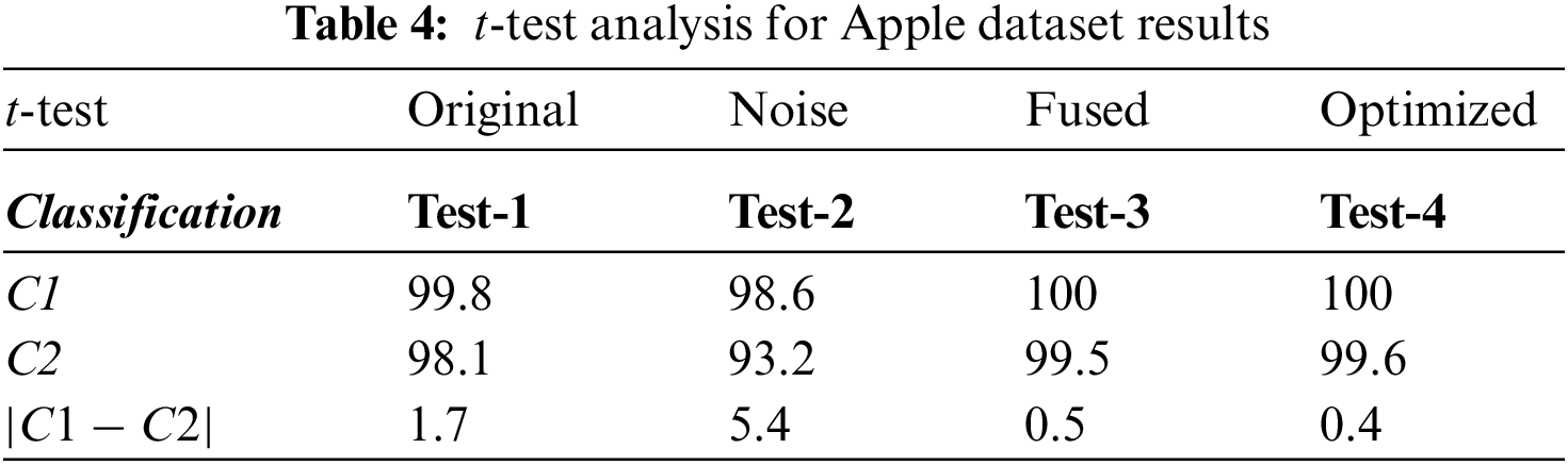
For this reason, ten different classifiers are used for evaluation, as mentioned in Table 3. The confusion matrix also proved the achieved accuracy rate through M-NN (Fig. 5). Diagonal values in the confusion matrix show the True Positive Rate (TPR). The values in Fig. 5 are clearly showing that the proposed approach shows improved TPR rates of 100%, 99.9%, 100%, and 100% for the Black Rot, Cedar Rust, healthy, and Scab classes of apple fruit diseases that are clearly showing the robustness of the proposed work. The t-test analysis is also computed, and values are noted in Table 4.

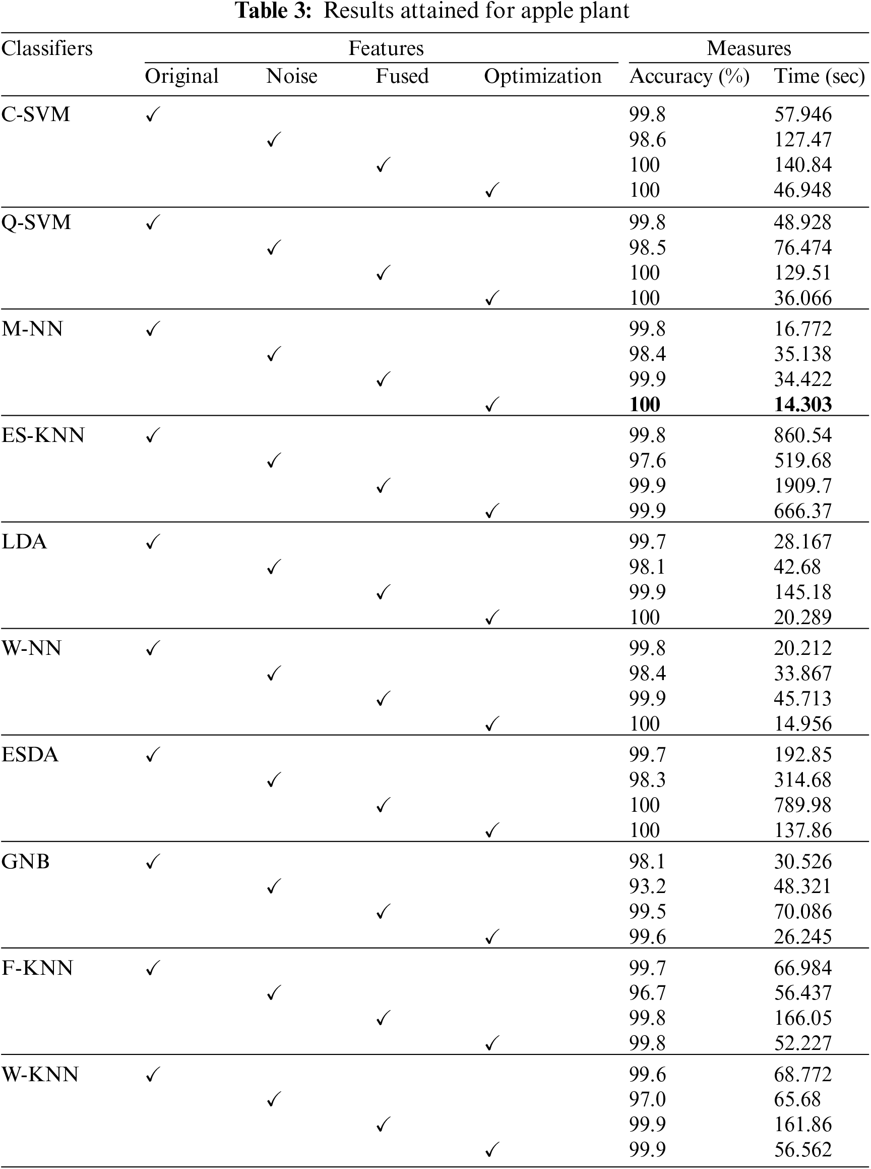
Figure 5: Confusion matrix for Apple dataset

After calculation mean value obtained is μ=2, standard deviation σ=2.32091, the value of t=1.72346, degree of freedom N−1=3, cumulative probability p=0.05 and Range =−3.182,+3.182.

Hypothesis: Value of t=1.72346 which lies in the range of −3.182,+3.182 of the two-tails test table. It shows that our t-test passed because the difference between the classifiers is very small.

4.2 Grapes Dataset Results

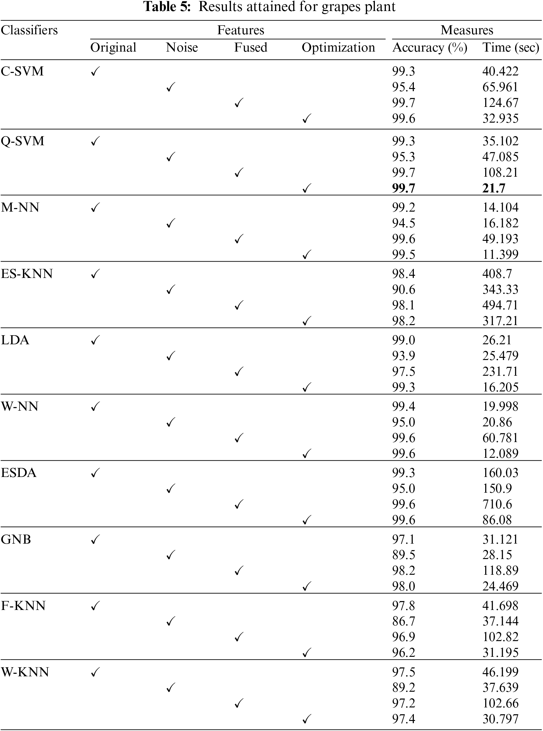
This section discussed the evaluation results of the proposed work for the grapes plant. The main statistical parameters used for evaluation are classification accuracy and training time. The grape dataset comprises four different classes, i.e., black rot, black measles, leaf blight, and healthy, which is used for model verification using 10-fold cross-validations. Ten different state-of-the-art classifiers are used for classification, and the results achieved are shown in Table 5. The values in Table 3 show that the highest classification accuracy is achieved by using a Quadratic Support Vector Machine (Q-SVM), i.e., 99.7% accuracy rate with a training time of 21.7 s. Wide and medium Neural Networks also achieved good accuracy rates, i.e., 97.4% and 99.7%. The major reason for improved classification accuracy is the PFA optimization technique, which extracts a nominative set of image features.

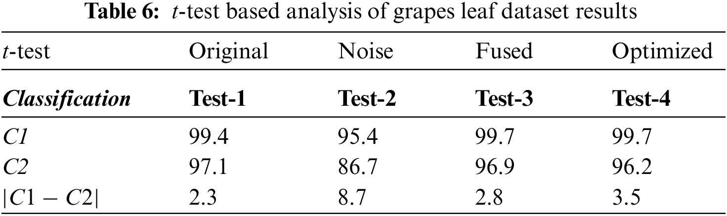
Moreover, the confusion matrix for classifying grape plant diseases is also given in Fig. 6. The values in Fig. 6 also prove the achieved results in which diagonal values show the True Positive Rates (TPR). The attained TPRs of 99.5%, 99.6%, 100%, and 99.5% for the Black Rot, Black Measles, Leaf Blight, and Healthy classes, respectively, exhibiting the proposed work’s effectiveness. The t-test-based analysis results are added under Table 6.

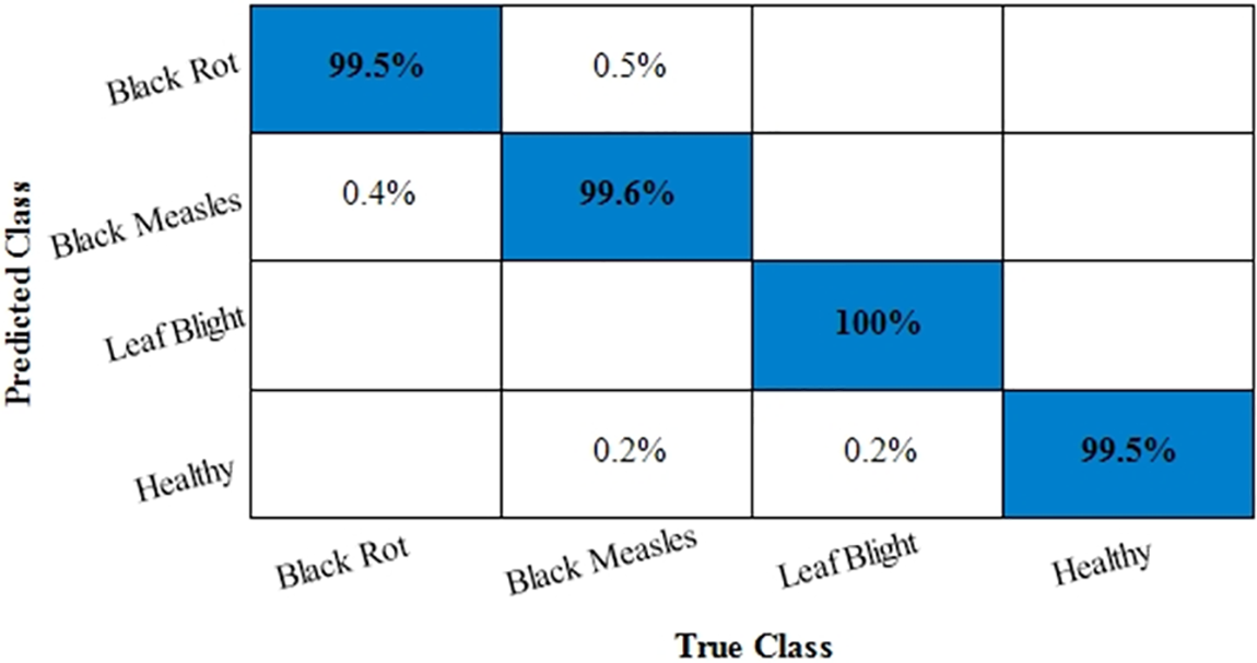
Figure 6: Confusion matrix for Grapes dataset

After calculation mean value obtained is μ=4.325, standard deviation σ=2.95789, value of t=2.92438, degree of freedom N−1=3, cumulative probability p=0.05 and Range =−3.182,+3.182.

Hypothesis: Value of t=2.92438 which lies in the range of −3.182,+3.182 of the two-tails test table. It shows that our t-test passed because the difference between the classifiers is very small.

4.3 Citrus Fruit Dataset Result

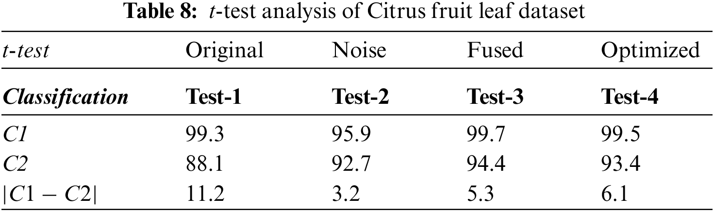
Next, classification performance of the proposed approach in recognizing the Citrus fruit diseases classification is presented. Accuracy and training time are the main statistical parameters used to test the proposed methodology. Three classes of Citrus fruit datasets, namely black spot, canker, greening, scab, and healthy, are considered for experimentation. The data is evaluated using 10-fold cross validations using ten different classifiers in Table 7. The highest accuracy rate is achieved on the Quadratic Support Vector Machine (Q-SVM), i.e., 99.7%, with a training time of 372.9 s. Medium and wide neural network classifiers also performed well in less training time. The accuracy in the case of citrus fruit is improved by using the fusion technique, i.e., features of original and noisy data are fused, and then classifiers are implemented. Such model description improves the recognition power of the proposed work. Further, the confusion matrix for the Citrus fruit is given in Fig. 7. It is quite visible from Fig. 7 that diagonal values in the confusion matrix showing the TPR depicts the high classification rate of the proposed approach. t-test results are given in Table 8.

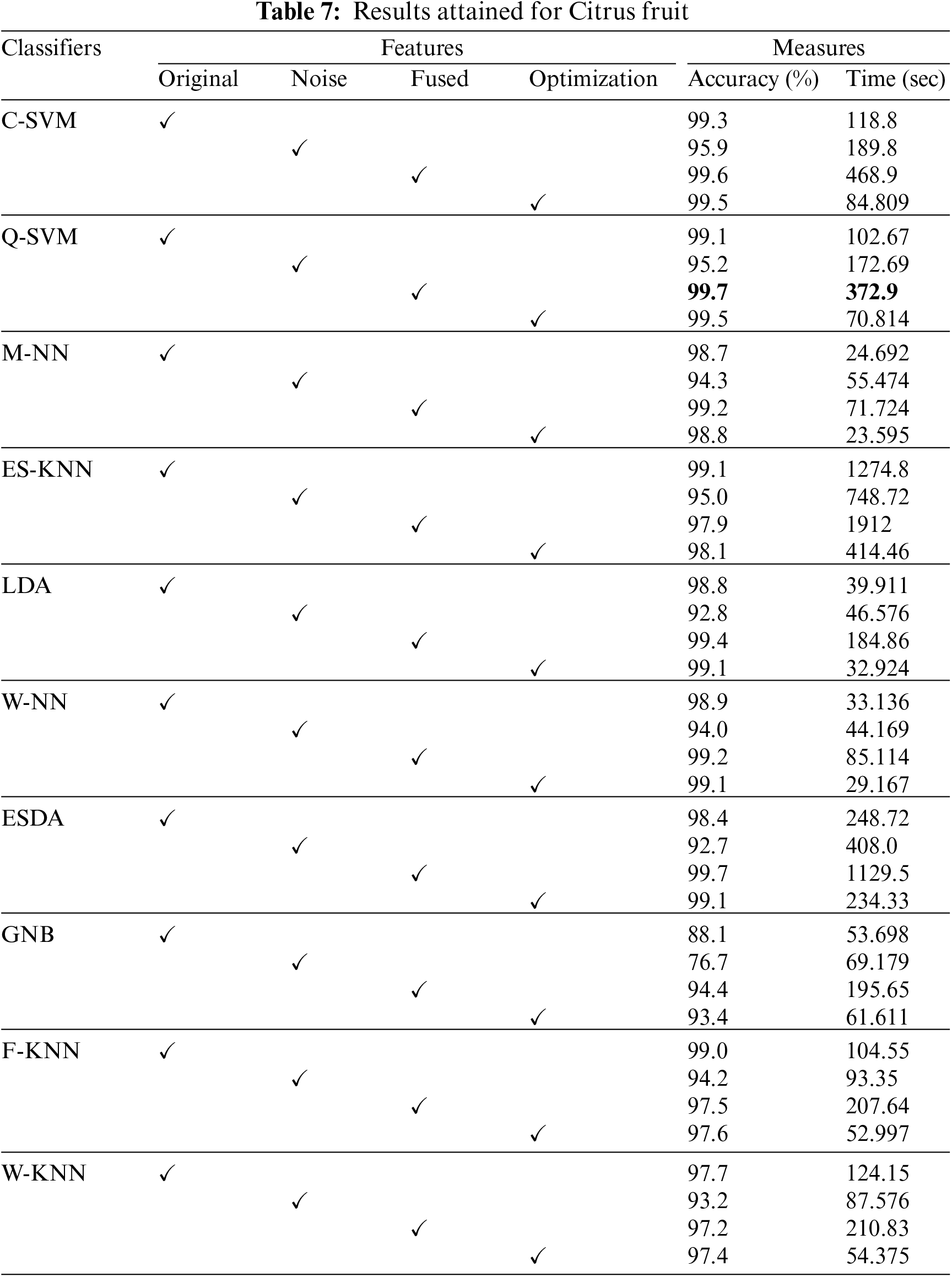
Figure 7: Confusion matrix for Citrus fruit dataset

After calculation mean value obtained is μ=6.45, standard deviation σ=3.39460, value of t=3.80015, degree of freedom N−1=3, cumulative probability p=0.05 and Range =−3.182,+3.182.

Hypothesis: Value of t=3.80015 which does not lie in the range of −3.182,+3.182 of the two-tails test table. It shows that our t-test failed because the difference between the classifiers is higher than the previous results.

4.4 Citrus Leaves Dataset Results

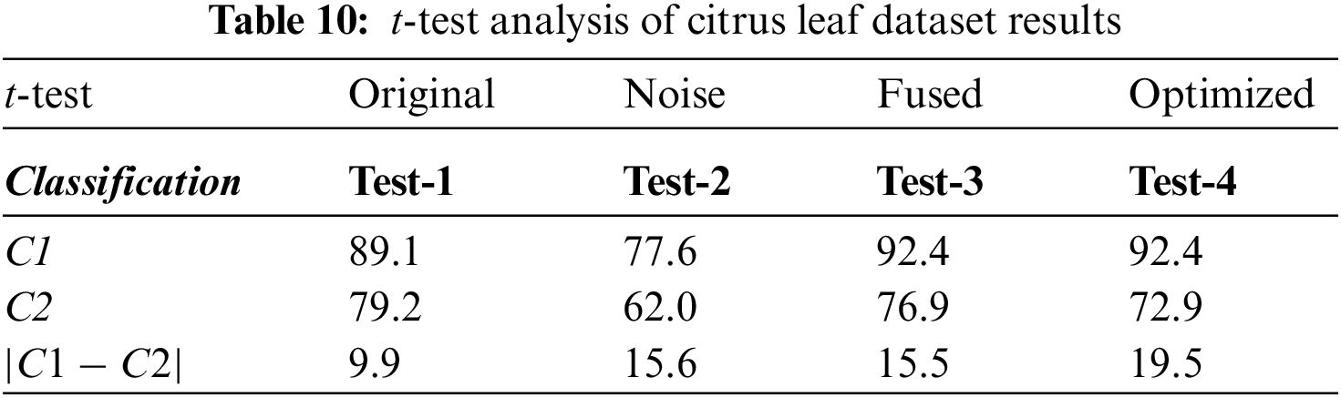
Next, an experiment is performed to validate the model’s effectiveness in recognizing the various diseases from the leaves images of the citrus plant. The two main statistical parameters for evaluation are accuracy and training time. In the case of Citrus leaves, five different classes, namely black spot, melanoses, greening, canker, and healthy, are used to evaluate the proposed methodology. Performance results for ten different classifiers are given in Table 9. The 10-fold cross-validations is employed on the available dataset. As a result, the highest accuracy rate is achieved M-NN, i.e., 93.4%, with a training time of 29.713 s for the fused feature set. Further, the confusion matrix for citrus plant leaves diseases is also given in Fig. 8. It is quite visible from Fig. 8 that diagonal values in the confusion matrix showing the TPR indicate the high recognition power of the introduced model to differentiate various abnormalities of the citrus plant leaves. Table 10 shows the analysis of the proposed accuracy.

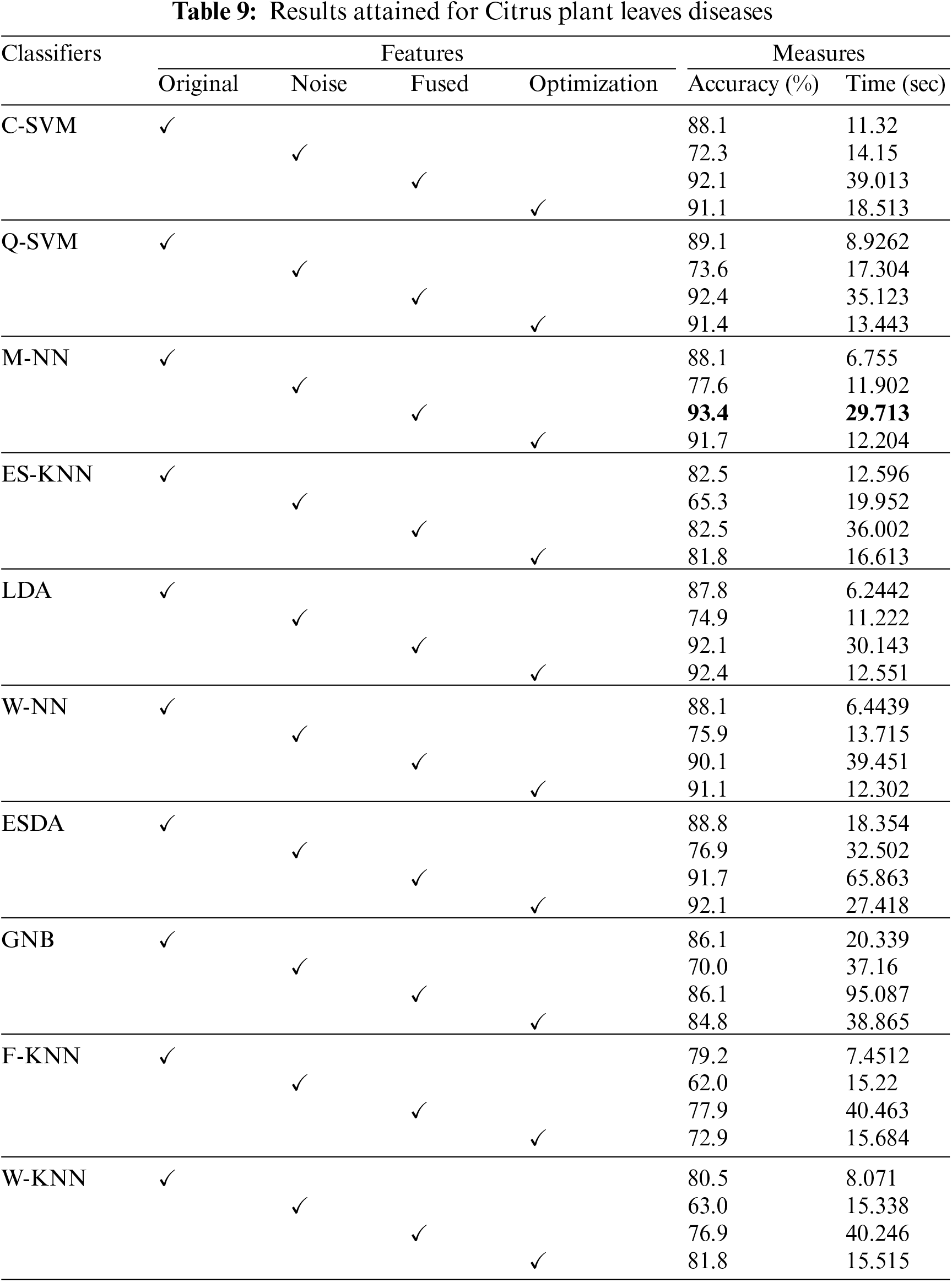
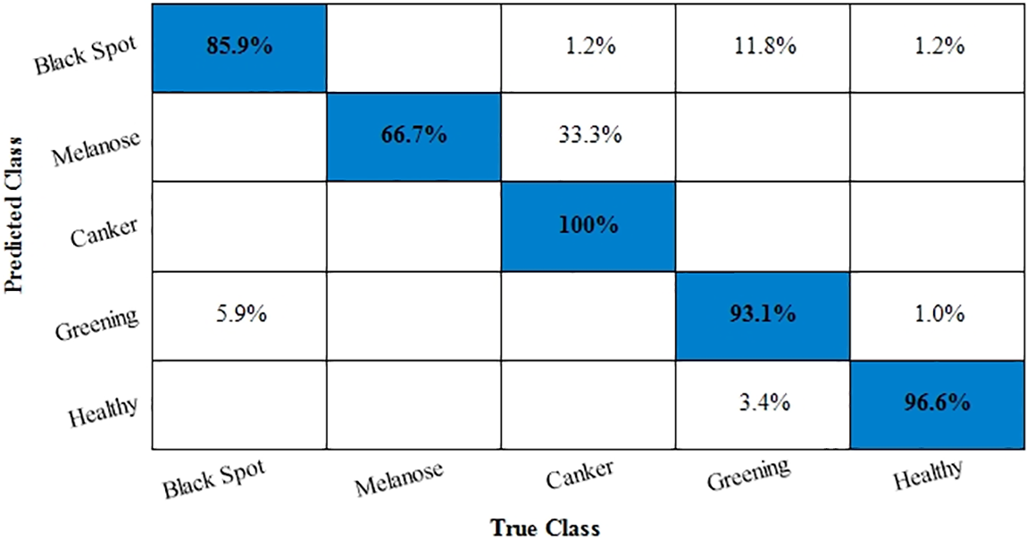
Figure 8: Confusion matrix for Citrus leaves dataset

After calculation mean value obtained is μ=15.15, standard deviation σ=3.95010, the value of t=7.67069, degree of freedom N−1=3, cumulative probability p=0.05 and Range =−3.182,+3.182.

Hypothesis: Value of t=7.67069 which does not lie in the range of −3.182,+3.182 of the two-tails test table. It shows that our t-test failed because of the reason that the difference between the classifiers is higher.

4.5 Comparison

Here, a comparison for all three fruit plants, namely apple, Citrus, and grapes, is performed with new approaches that attempt to solve the same problem. The attained comparison is given in Table 11. Sun et al. [45] presented a CNN-based model for classifying common apple diseases. Experimental results show 83.12% classification accuracy, depicting the model’s efficiency and accurate disease classification. Gu et al. [30] presented an improved CNN-based model for accurately classifying commonly occurring apple diseases. Badjie et al. [46] presented a framework for grape disease classification and obtained an accuracy rate of 97.75% after the experimentation. Paymode et al. [47] proposed a Convolutional Neural Network based Visual Geometry Group (VGG) model and obtained the highest accuracy value of 99.7%. Tiwari et al. [48] discussed automatic plant leaves detection using Deep Convolutional Neural Networks (DCNN). Elaraby et al. [49] discussed the difficulties observed during the manual detection of plant diseases because only plant pathologists can classify diseases with the naked eye, which is also sometimes a complex task. They used AlexNet and VGG-19, two pre-trained models, for accurate classification and obtained an accuracy of 99.7%. Syed-Ab-Rahman et al. [31] presented a faster R-CNN two-stage CNN-based model and obtained 94.37% accuracy. Khattak et al. [50] presented a CNN-based model and achieved 94.55% accuracy. In the proposed framework, the obtained accuracy of 100%, 99.7%, 99.7%, and 93.4% for Apple, Grapes, Citrus fruits, and Citrus leaves datasets, respectively. Moreover, the visual analysis is conducted through Grad-CAM visualization, as shown in Fig. 9. From this figure, it is clearly observed that the proposed framework diagnosis of disease region is well and also shows the importance of better trained deep models.

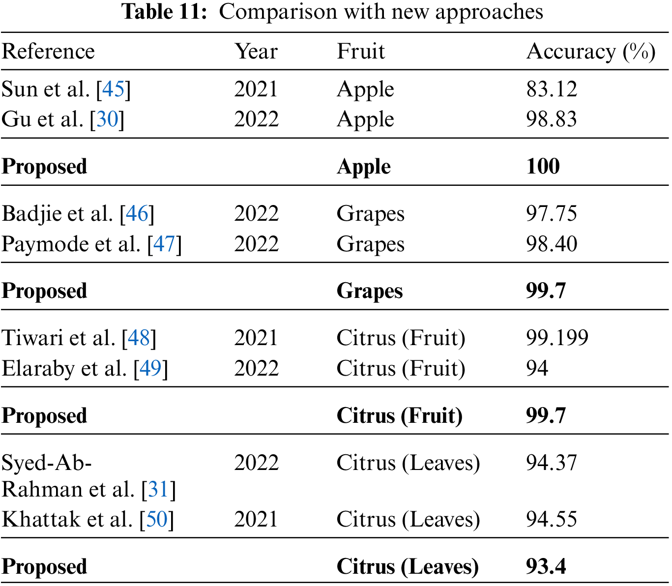
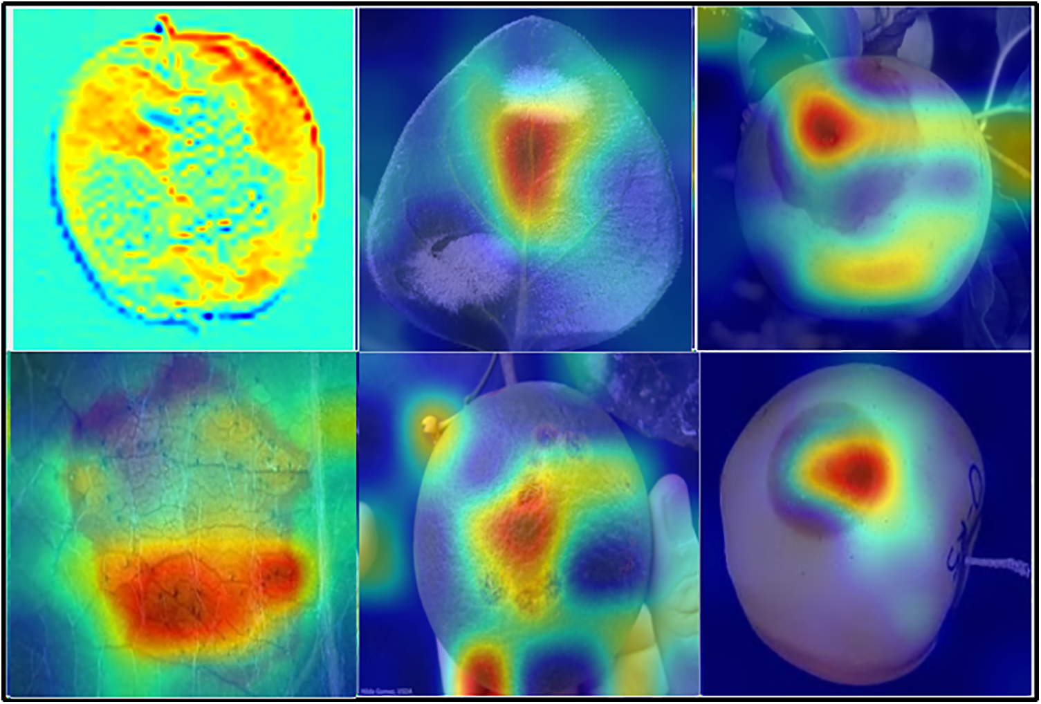
Figure 9: Grad-CAM based visualization of the proposed framework

5  Conclusion

Using the concept of feature fusion with key point optimization, an automated method for classifying diseases of three different types of fruits is provided in this study. All three fruit categories’ photos are first gathered and given original data names. After that, numerous artifacts are added to the original dataset and given the moniker “noisy data.” Transfer learning is then utilized to apply the EfficientNet-B0 Deep Convolutional Neural Network model to the original and noisy data, computing representative and non-redundant features later fused to obtain features from both the original and noisy data. Finally, employing a variety of classifiers, including the Medium Neural Network, Wide Neural Network, Support Vector Machine, and others, the PFA optimization technique creates a collection of optimized features that are then categorized. As a result, it is observed that the suggested fusion technique boosts processing effectiveness while improving prediction performance.

Additionally, the optimization stage helps shorten testing times while keeping classification accuracy. Future researchers will propose a CNN-based model and recommend Bayesian optimization to optimize the model hyperparameters. Additionally, a few effective learning strategies and fresh keypoint nomination methods will be used.

Acknowledgement: This work was supported by the “Human Resources Program in Energy Technology” of the Korea Institute of Energy Technology Evaluation and Planning (KETEP) and granted financial resources from the Ministry of Trade, Industry, and Energy, Korea.

Funding Statement: This work was supported by the “Human Resources Program in Energy Technology” of the Korea Institute of Energy Technology Evaluation and Planning (KETEP) and granted financial resources from the Ministry of Trade, Industry, and Energy, Korea (No. 20204010600090).

Author Contributions: The authors confirm contribution to the paper as follows: study conception and design: I.H, M.A.K, and M.N; data collection: I.H, M.A.K, and T.K; draft manuscript preparation: I.H, M.A.K, and M.N; funding: T.K and J.C; validation: T.K and J.C; software: I.H, M.A.K, and T.K; visualization: M.N and J.C; supervision: M.A.K, M.N and J.C. All authors reviewed the results and approved the final version of the manuscript.

Availability of Data and Materials: The dataset used in this work is publically available for research purpose (https://www.kaggle.com/datasets/emmarex/plantdisease).

Conflicts of Interest: The authors declare that they have no conflicts of interest to report regarding the present study.

References

1. C. Gao, “Genome engineering for crop improvement and future agriculture,” Cell, vol. 184, no. 6, pp. 1621–1635, 2021. [Google Scholar] [PubMed]

2. Z. Tian, J. W. Wang, J. Li and B. Han, “Designing future crops: Challenges and strategies for sustainable agriculture,” The Plant Journal, vol. 105, no. 2, pp. 1165–1178, 2021. [Google Scholar] [PubMed]

3. A. Kader, “Importance of fruits, nuts, and vegetables in human nutrition and health,” Perishables Handling Quarterly, no. 106, pp. 4–6, 2001. [Google Scholar]

4. Z. Tang, Z. Zhao, X. Wu and W. Lin, “A review on fruit and vegetable fermented beverage-benefits of microbes and beneficial effects,” Food Reviews International, vol. 6, no. 2, pp. 1–38, 2022. [Google Scholar]

5. G. Fenu and F. M. Malloci, “Forecasting plant and crop disease: An explorative study on current algorithms,” Big Data and Cognitive Computing, vol. 5, no. 1, pp. 2, 2021. [Google Scholar]

6. S. Sangeetha, M. Sudha, R. Balamanigandan and V. Pushparathi, “Comparison of crop disease detection methods-an intensive analysis,” Psychological Education, vol. 58, no. 12, pp. 10540–10546, 2021. [Google Scholar]

7. L. Hartley, E. Igbinedion, J. Holmes and N. Flowers, “Increased consumption of fruit and vegetables for the primary prevention of cardiovascular diseases,” Cochrane Database of Systematic Reviews, vol. 15, no. 4, pp. 1–15, 2013. [Google Scholar]

8. R. Zhu, H. Zou, Z. Li and R. Ni, “Apple-Net: A model based on improved YOLOv5 to detect the apple leaf diseases,” Plants, vol. 12, no. 4, pp. 169, 2023. [Google Scholar]

9. X. Wang, J. Liu and X. Zhu, “Early real-time detection algorithm of tomato diseases and pests in the natural environment,” Plant Methods, vol. 17, no. 4, pp. 1–17, 2021. [Google Scholar]

10. S. Thomas, M. T. Kuska, D. Bohnenkamp and A. Brugger, “Benefits of hyperspectral imaging for plant disease detection and plant protection: A technical perspective,” Journal of Plant Diseases and Protection, vol. 125, no. 2, pp. 5–20, 2018. [Google Scholar]

11. N. C. Eli-Chukwu, “Applications of artificial intelligence in agriculture: A review,” Engineering, Technology & Applied Science Research, vol. 9, no. 7, pp. 4377–4383, 2019. [Google Scholar]

12. M. Ouhami, A. Hafiane, Y. Es-Saady, M. El Hajji and R. Canals, “Computer vision, IoT and data fusion for crop disease detection using machine learning: A survey and ongoing research,” Remote Sensing, vol. 13, no. 6, pp. 2486, 2021. [Google Scholar]

13. S. Sood and H. Singh, “Computer vision and machine learning based approaches for food security: A review,” Multimedia Tools and Applications, vol. 21, no. 5, pp. 1–27, 2021. [Google Scholar]

14. J. Chen, J. Chen, D. Zhang, Y. A. Nanehkaran and Y. Sun, “A cognitive vision method for the detection of plant disease images,” Machine Vision and Applications, vol. 32, no. 5, pp. 1–18, 2021. [Google Scholar]

15. A. Yousuf and U. Khan, “Ensemble classifier for plant disease detection,” Multimedia Tools and Applications, vol. 20, no. 4, pp. 1–27, 2021. [Google Scholar]

16. A. Likas, N. Vlassis and J. J. Verbeek, “The global k-means clustering algorithm,” Pattern Recognition, vol. 36, no. 2, pp. 451–461, 2003. [Google Scholar]

17. S. Bashir and N. Sharma, “Remote area plant disease detection using image processing,” IOSR Journal of Electronics and Communication Engineering, vol. 2, no. 11, pp. 31–34, 2012. [Google Scholar]

18. S. Kumar and R. Kaur, “Plant disease detection using image processing–A review,” International Journal of Computer Applications, vol. 124, no. 21, pp. 1–11, 2015. [Google Scholar]

19. J. Liu and X. Wang, “Plant diseases and pests detection based on deep learning: A review,” Plant Methods, vol. 17, no. 2, pp. 1–18, 2021. [Google Scholar]

20. J. A. Wani, S. Sharma, M. Muzamil, S. Ahmed and S. Singh, “Machine learning and deep learning based computational techniques in automatic agricultural diseases detection: Methodologies, applications, and challenges,” Archives of Computational Methods in Engineering, vol. 12, no. 2, pp. 1–37, 2021. [Google Scholar]

21. M. Nimbarte, M. Pal, S. Sonekar and P. Ulhe, “Some effective techniques for recognizing a person across aging,” Evolutionary Computing and Mobile Sustainable Networks, vol. 3, no. 1, pp. 69–77, 2021. [Google Scholar]

22. A. Kamilaris and F. X. Prenafeta-Boldú, “Deep learning in agriculture: A survey,” Computers and Electronics in Agriculture, vol. 147, no. 6, pp. 70–90, 2018. [Google Scholar]

23. J. Padmapriya and T. Sasilatha, “Deep learning based multi-labelled soil classification and empirical estimation toward sustainable agriculture,” Engineering Applications of Artificial Intelligence, vol. 119, no. 8, pp. 105690, 2023. [Google Scholar]

24. P. Bansal, R. Kumar and S. Kumar, “Disease detection in apple leaves using deep convolutional neural network,” Agriculture, vol. 11, no. 2, pp. 617, 2021. [Google Scholar]

25. R. Thapa, K. Zhang, N. Snavely, S. Belongie and A. Khan, “The plant pathology challenge 2020 data set to classify foliar disease of apples,” Applications in Plant Sciences, vol. 8, no. 4, pp. e11390, 2020. [Google Scholar] [PubMed]

26. L. Perez and J. Wang, “The effectiveness of data augmentation in image classification using deep learning,” Archives of Computational Methods in Engineering, vol. 12, no. 2, pp. 1–37, 2017. [Google Scholar]

27. J. Canny, “A computational approach to edge detection,” IEEE Transactions on Pattern Analysis and Machine Intelligence, vol. 14, no. 2, pp. 679–698, 1986. [Google Scholar]

28. L. Li, S. Zhang and B. Wang, “Apple leaf disease identification with a small and imbalanced dataset based on lightweight convolutional networks,” Sensors, vol. 22, no. 4, pp. 173, 2021. [Google Scholar] [PubMed]

29. J. Di and Q. Li, “A method of detecting apple leaf diseases based on improved convolutional neural network,” PLoS One, vol. 17, no. 3, pp. e0262629, 2022. [Google Scholar] [PubMed]

30. Y. H. Gu, H. Yin, D. Jin, R. Zheng and S. J. Yoo, “Improved multi-plant disease recognition method using deep convolutional neural networks in six diseases of apples and pears,” Agriculture, vol. 12, no. 14, pp. 284–300, 2022. [Google Scholar]

31. S. F. Syed-Ab-Rahman, M. H. Hesamian and M. Prasad, “Citrus disease detection and classification using end-to-end anchor-based deep learning model,” Applied Intelligence, vol. 52, no. 6, pp. 927–938, 2022. [Google Scholar]

32. A. Ajit, K. Acharya and A. Samanta, “A review of convolutional neural networks,” in 2020 Int. Conf. on Emerging Trends in Information Technology and Engineering (ic-ETITE), NY, USA, pp. 1–5, 2020. [Google Scholar]

33. W. H. L. Pinaya, S. Vieira, R. Garcia-Dias and A. Mechelli, “Convolutional neural networks,” Machine Learning, vol. 21, no. 4, pp. 173–191, 2021. [Google Scholar]

34. Y. D. Zhang, S. C. Satapathy and S. H. Wang, “Improved breast cancer classification through combining graph convolutional network and convolutional neural network,” Information Processing & Management, vol. 58, no. 8, pp. 102439, 2021. [Google Scholar]

35. D. R. Nayak, D. Das, R. Dash, S. Majhi and B. Majhi, “Deep extreme learning machine with leaky rectified linear unit for multiclass classification of pathological brain images,” Multimedia Tools and Applications, vol. 79, no. 3, pp. 15381–15396, 2020. [Google Scholar]

36. J. Teuwen and N. Moriakov, “Convolutional neural networks,” Handbook of Medical Image Computing and Computer Assisted Intervention, vol. 11, no. 2, pp. 481–501, 2020. [Google Scholar]

37. A. Khan, A. Sohail, U. Zahoora and A. S. Qureshi, “A survey of the recent architectures of deep convolutional neural networks,” Artificial Intelligence Review, vol. 53, no. 15, pp. 5455–5516, 2020. [Google Scholar]

38. M. Lin, Q. Chen and S. Yan, “Network in network,” Information Processing & Management, vol. 28, no. 6, pp. 102439, 2013. [Google Scholar]

39. J. Deng, W. Dong, R. Socher, K. Li and F. F. Li, “ImageNet: A large-scale hierarchical image database,” in 2009 IEEE Conf. on Computer Vision and Pattern Recognition, NY, USA, pp. 1–8, 2020. [Google Scholar]

40. M. Tan and Q. Le, “Efficientnet: Rethinking model scaling for convolutional neural networks,” in Int. Conf. on Machine Learning, NY, USA, pp. 6105–6114, 2019. [Google Scholar]

41. K. He, X. Zhang, S. Ren and J. Sun, “Deep residual learning for image recognition,” in Proc. of the IEEE Conf. on Computer Vision and Pattern Recognition, NY, USA, pp. 770–778, 2016. [Google Scholar]

42. S. Zagoruyko and N. Komodakis, “Wide residual networks,” Sensors, vol. 21, no. 2, pp. 1–21, 2016. [Google Scholar]

43. K. Weiss, T. M. Khoshgoftaar and D. Wang, “A survey of transfer learning,” Journal of Big Data, vol. 3, no. 11, pp. 1–40, 2016. [Google Scholar]

44. H. Yapici and N. Cetinkaya, “A new meta-heuristic optimizer: Pathfinder algorithm,” Applied Soft Computing, vol. 78, no. 21, pp. 545–568, 2019. [Google Scholar]

45. H. Sun, H. Xu, B. Liu, D. He and J. He, “MEAN-SSD: A novel real-time detector for apple leaf diseases using improved light-weight convolutional neural networks,” Computers and Electronics in Agriculture, vol. 189, no. 5, pp. 106379, 2021. [Google Scholar]

46. B. Badjie and E. D. Ülker, “A deep transfer learning based architecture for brain tumor classification using MR images,” Information Technology and Control, vol. 51, no. 4, pp. 332–344, 2022. [Google Scholar]

47. A. S. Paymode and V. B. Malode, “Transfer learning for multi-crop leaf disease image classification using convolutional neural network VGG,” Artificial Intelligence in Agriculture, vol. 6, no. 5, pp. 23–33, 2022. [Google Scholar]

48. V. Tiwari, R. C. Joshi and M. K. Dutta, “Dense convolutional neural networks based multiclass plant disease detection and classification using leaf images,” Ecological Informatics, vol. 63, no. 4, pp. 101289, 2021. [Google Scholar]

49. A. Elaraby, W. Hamdy and S. Alanazi, “Classification of citrus diseases using optimization deep learning approach,” Computational Intelligence and Neuroscience, vol. 2022, no. 14, pp. 1–21, 2022. [Google Scholar]

50. A. Khattak, M. U. Asghar, U. Batool and M. Z. Asghar, “Automatic detection of citrus fruit and leaves diseases using deep neural network model,” IEEE Access, vol. 9, no. 3, pp. 112942–112954, 2021. [Google Scholar]