Optimal Energy Consumption Optimization in a Smart House by Considering Electric Vehicles and Demand Response via a Hybrid Gravitational Search and Particle Swarm Optimization Algorithm

Nomenclature

1  Introduction

Most industrial and developing countries have recently paid attention to energy loss prevention in residential buildings. This issue has found more significance with the rising demands for oil and oil-generated energy. The need for new residential, administrative, educational, and other buildings and the tendency to use new equipment has increased energy consumption in this sector. The global energy loss statistics show that wasteful energy consumption is higher in residential and commercial buildings than in other sectors. Currently, almost 40% of the total energy consumed worldwide belongs to the residential and commercial sectors [1]. Building automation and management systems have had remarkable achievements in reducing construction industry costs and decreasing and optimizing energy consumption. For better and more reasonable energy savings, there is a dire need for building smartization and precise control systems in buildings. Building management systems (BMS) are installed in buildings to control different parts of the building via their components [2]. These systems aim to adapt the operation of different components to the needs of the building, its residents, and the environmental conditions at the time. Various sensors inside and outside buildings and a unified system can control all welfare and security conditions in real-time. This way, energy losses are controlled and used to achieve an ideal condition [3]. Building smartization systems provide all these items for the residents to better exploit building spaces [4]. At present, smart houses mainly focus on demand response (DR) strategies and the interaction between generation companies and consumers. DR refers to a change in electrical energy consumption on the consumers’ part in response to a change in electricity price or incentives offered for electricity consumption reduction in peak hours [5].

In the DR process, end-users change their consumption pattern in response to electricity price variations at different times. In other words, they manage and program their consumption. To motivate the end-users to manage their consumption then, incentives are offered to them in addition to reducing their electricity costs [6]. All these processes promote grid confidence during faults. This definition shows that DR programs mainly aid power systems during peak hours. They motivate the consumers to re-program their consumption patterns. These programs have recently become very popular in modern electric power systems. Overall, DR aims to decrease electricity consumption in peak hours when the energy purchasing price on the market is very high or the system’s storage level is low due to possible events. Home energy management systems (HEMS) and smart measuring infrastructure play a vital role in the effectiveness of DR strategies in residential areas [7]. Optimal programming of appliances is an effective home energy management method that can decrease energy costs and peak demands. With the emergence of smart grids in recent years, various studies have been conducted on load programming, DR, and their optimization in smart houses, which will be reviewed below. In [8], an integrated framework was proposed for DR to resolve the existing deficiencies. First, an analysis of the household energy consumption data, a controllable system, and DR were taken into account. Then, the energy consumption pattern was reduced by using flexible load models and better use of ESS. In [9], an efficient and cost-effective EMS was implemented in smart industrial grids, focusing on the increasing tendency in electric load consumption and constraints on increasing the electricity power station capacity. Next, the optimal programming was performed by using the existing energy sources along with the DR program, EVs in the parking lot, and EMS in the smart industrial grids. In [10], a DR strategy was proposed based on the user-expected price for a smart house with an ESS to minimize the energy consumption costs. In [11], a HEMS was introduced by considering DR and dispersed generation (DG) sources in modeling. Household electricity demand, EVs, BESS, and different non-time-shiftable devices were present in the system. In [12], the effect of efficient DR in a smart grid was noted for energy balance. It was stated that efficient management could reduce the national electricity grid load and minimize the local operational electricity costs. In [13], a novel demand-side management method was proposed for programming the operation of home appliances to minimize energy supply costs by considering time-variable energy prices. Due to the uncertainty in predicting home appliances’ performance, and solar RES generation, stochastic programming was conducted by considering the energy adjustment variable β to model the uncertainty in time and appliance energy consumption. In [14], the performance of a smart house was dealt with in the presence of EVs, solar panels, and time-shiftable loads. In [15], DR optimization was formulated as a linear optimization problem to minimize the household bills and the waiting time for appliances. In [16], the consumption of different appliances in a household at different free times was determined to minimize the maximum hourly load. DR optimization was formulated as a linear optimization problem solved by MILP. A considerable decrease was obtained in the household peak hourly load. Moreovera more balanced hourly load can be attained by using several households in the DR program. In [17], the optimal charge/discharge pattern and BESS capacity were determined in smart house energy management with a solar system using an optimal metaheuristic algorithm and stochastic mixed-integer nonlinear programming (MINLP) and by taking into account uncertainty in solar-generated power prediction. In [18], MinLP was used to solve the residential DR optimization problem. The optimal on/off status of 10 household appliances at 10-min free times for a 24-h horizon was obtained in the DR program. The daily bill and consumer problems were minimized for an optimization problem with several binary decision variables. In [19], a smart household management method was proposed for houses with a solar energy generation system and ESS. The house’s consumed energy was predicted by using neural networks. In [20], the optimal performance of a smart HEM system in coordinating and integrating the appliances was examined to promote the productivity and economic advantages of the smart home.

Less time for the charging model is presented in [21] by balancing total consumption without any discomfort of drivers. In this approach, the owners of EVs should fill in an information sheet which consists of the number and lengths of their next. A holistic approach to optimizing the use of various home appliances based on the prosumers’ preferences and defined schedules is presented in [22]. The Peer-to-Peer (P2P) energy trading role in system operation is presented in [23], which is considered in various test cases by four prosumer approaches considering Energy Storage Systems (ESS), Photovoltaic (PV), and EV. The ESS placement is presented in [24] based on residential buildings by considering the mutual benefits of investors and users. Optimal load dispatch from the energy hub to reduce the total costs of the energy hub, i.e., exploitation and emission costs, is presented in [25]. The presented energy hub consists of combined heat and power (CHP), PV, wind turbine (WT), and EV. The Monte Carlo simulation approach has been considered in the modeling of this system by considering future uncertainties in electricity prices.

The imprecise prediction of RES-generated power would certainly lead to non-optimal HEM (energy storage programming, EV charge/discharge management, energy sales/purchase to/from the grid, appliance on/off programming, etc.). Non-optimal energy management and programming also increase household electricity costs, thereby limiting the advantages of home smartization. Therefore, stochastic programming and considering the uncertainties lead to better programming. Moreover, by using the risk criterion, considerable variations in-home energy supply costs in different scenarios can be managed so that the consumer does not face great variations in costs and the expected costs can be reduced.

None of the reviewed papers have comprehensively proposed an energy supply cost-restrained linear model for smart HEM by considering EV charge/discharge programming, DR program, solar RES, and ESS for predicting solar-generated power prediction uncertainty. Therefore, the present paper aims to propose a model to consider the factors mentioned above. So, the contributions of this paper can be summarized as follows:

•   Solving the optimal energy consumption problem by considering the electric vehicles and demand response in smart homes.

•   Application of hybrid gravitational search and particle swarm optimization algorithm for solving the mentioned problem.

•   Considering the solar RES and ESS for predicting solar-generated power prediction uncertainty.

1.1 Smart Houses

In smart houses, residential buildings are combined with smart technologies to promote safety, electricity consumption optimization and users’ welfare. Users in these houses can control and monitor the HEMS and smart appliances from a distance; in other words, HEMS is a distant monitoring system using distance communication technology. This system includes hardware and software that allow users to effectively manage their electricity consumption by controlling the time of using smart appliances.

1.1.1 Smart House Structure and Model

A smart house must be equipped with a HEMS, which consists of hardware and software, e.g., smart meters. Smart meters receive and dispatch signals to electricity supply companies. Electricity supply companies transfer price signals to smart meters through the data network. Then, smart meters dispatch the price signals to energy management controllers (EMC) and send users’ feedback to the companies. An EMC is the core of HEMS. Through sensors installed in appliances, EMC allows users to connect to smart appliances by using smartphone apps [26].

2  System Description and Method

A smart HEMS aims to minimize the daily energy consumption costs by meeting all the system constraints. The total cost is defined as the difference between the cost of the energy purchased from the grid and the revenues resulting from selling energy to the grids (Eq. (1)). To constrain cost variations in different scenarios then, the conditional value at risk (CVaR) criterion is used:

Cost=(1−β)∑t∑sρs[PtsgridΔTλtsell]+βCVAR(1)

where Cost is the building’s daily energy consumption cost, ρs is the probability of occurrence of the s th scenario, ΔT is the programming interval, CVAR is the CVaR and β is the weight coefficient for the risk criterion. The value of CVAR is defined in Eqs. (2) and (3):

CVAR=η+11−α∑sρsξs(2)

∑t[PtsgridΔTλtbuy−PtssoldΔTλtsell]−η≤ξ(s)(3)

where η, α and ξ are recourse variables to calculate the risk criterion CVAR. The objective function must be optimized based on the following constraints.

2.1 Power Balance

In any electric system, the balance between the generated and consumed power must hold as follows [4]:

Ptsgrid+PtsPV,used+PtsEV,dis+PtsESS,dis=PtsEV,ch+PtsESS,ch+Ptother+∑mPmtssh∀t,s(4)

Generated power comprises the power purchased from the grid, solar power, EV discharge power, and ESS power. Consumed power comprises constant load demands, EV charge power, ESS charge and shiftable loads’ consumed power. This constraint must hold for all the intervals and scenarios.

2.2 ESS Modeling

With the increased penetration of RES in electricity grids and the transformation of inactive distribution networks into active ones, it is essential to aggregate these resources to promote participation and visibility and to create a proper mediator between these sources and the electricity grid. The battery energy storage system (BESS) is an accessible resource greatly contributing to peak shaving, usable voltage quality, and active force adjustment capacity. Batteries are among the most frequently used chargeable reservoirs of different sizes and designs. The main attribute of BESS is its low costs and low self-discharge. Batteries are incorporated to store the surplus energy generated by the system and supply the additional power demanded by loads. Batteries can be set to a state of charge or discharge, depending on the system’s performance. The input power of batteries can be positive or negative, depending on the charge/discharge performance. Technical constraints of BESS are presented below. The following equations demonstrate the initial battery energy and the minimum and maximum energy storage levels in the battery [4].

SOCt=SOCinitial(5)

SOCt≤SOCmax(6)

SOCt≥SOCmin(7)

The minimum and maximum battery charge and discharge constraints are presented below:

Ptcharge≤Pchargemax×Utcharge(8)

Ptcharge≥Pchargemin×Utcharge(9)

Ptdisk≤Pdiskmax×Utdisk(10)

Ptdisk≥Pdiskmin×Utdisk(11)

The battery cannot simultaneously be charged and discharged. This constraint is formulated below:

Utcharge+Utdisk≤1(12)

The dynamic model of battery energy is calculated via:

SOCt=SOCt−1+ηchB×Ptcharge−PtdiskηdiskB(13)

2.3 EV Modeling

EVs utilize a battery with considerable capacity; therefore, the EV model is assumed to be similar to the battery model. The mathematical modeling of EVs resembles that of the ESS system with the difference that EVs are in the parking lot at certain and limited times, while the BESS constantly participates in the HEM program. Moreover, as the homeowner also owns the EV and the optimization program is solved for the next 24 h, the EV owner almost precisely knows the daily EV use in the next 24 h. Therefore, the uncertainty in predicting the time of EV’s presence in the parking lot is not taken into account [27].

Constraints on EV modeling are described below:

PtsEV,ch≤CREVutEVZtEV∀t,s(14)

PtsEV,dis≤DREV(1−utEV)ZtEV∀t,s(15)

SOEtsEV=SOEt−1sEV+CEEVPtsEV,chΔT−PtsEV,DISΔT∀t≠tent,s(16)

SOEtentsEV=SOEEV,ini∀s(17)

ZtEVSOEEV,ini≤SOEtsEV≤ZtEV,max∀t,s(18)

SOEtdepsEV≥MSOEEV,max(19)

In Eqs. (14) and (15), the EV battery charge and discharge power is constrained at the hours when the EV is in the parking lot. Eq. (16) calculates the EV battery’s charge level at the hours when the EV is in the parking lot. Based on Eq. (17), when the EV enters the parking lot, it has a certain level of energy. Constraint (18) specifies the minimum and maximum permissible levels of EV energy. Constraint (19) allows the homeowner to determine an optional EV charge level when exiting the house.

2.4 Solar Panel Model

The power generated by solar panels supplies the internal needs of the building; if there is surplus power, it can be sold to the upstream grid:

PtsPV=PtsPV,used+PtsPV,sold∀t,s(20)

Ptssold=Ptspv,sold∀t,s(21)

Based on Eq. (20), solar power can supply the internal uses of the building and be sold to the grid. In this paper, the surplus amount of power generated by solar panels can be sold to the upstream grid (Eq. (21)).

2.5 Power Exchange with the Upstream Grid

A smart building is connected to the upstream grid via a feeder with thermal constraints. Therefore, the power purchased from/sold to the upstream grid should not exceed the feeder’s thermal limit or the value mentioned in the contract.

Ptsgrid≤N1utgrid∀t,s(22)

Ptssild≤N(1−utgrid)∀t,s(23)

Based on Constraints (22) and (23), if the building is receiving power from the upstream grid, the sold power must be 0. Similarly, if the building is selling power, the power entering from the grid must be 0. Values of N1 and N2 parameters are determined by the agreed-upon framework between the building energy supplier and the owner.

2.6 Household Loads

To better model the household appliances, they are classified based on the method of usage into three groups: flexible loads, appliances with the stochastic time of use (STOU), and weather-related loads (WRLs). Flexible loads have a predictable and routine time of use (TOU) and follow a specific behavioral pattern, e.g., washing machines, dishwashers, and electric water boilers. The TOU of loads with the stochastic TOU depends on unpredictable factors and conditions and does not follow a specific behavior pattern, e.g., televisions, computers, and lighting.

Weather-related loads are a type of inflexible loads with weather-related consumption. Simply put, weather parameter determines the consumption of these loads, e.g., refrigerators, ventilation systems, and water heaters.

2.6.1 Flexible Load Modeling

The following method is adopted in this study to model the consumption pattern of flexible loads. First, any flexible appliance is defined as Euj. Then, the appliance is assumed to consume the energy of Uj every time it is turned on. We also assume this flexible appliance consumes this amount of energy within [Aj, Bj] and is plugged in. In this interval, Aj stands for the time of plug-in and Bj for the time of plug-out. Based on these assumptions and determining the nature of the defined parameters, the flexible loads are modeled as follows:

Uj=∑n=Ajn=BjEEujh,{[Aj,Bj]∈n,Aj<Bj}(24)

For each flexible appliance, we define minimum and maximum hourly energy consumptions, specified as DjMin and DjMax, respectively. Based on the mentioned hourly energy consumption levels, the DR program by the consumer is expressed as:

Djmin≤Ejh≤Djmax,h=Aj,Aj+1,…,Bj−1,Bj(25)

where Ejh indicates the consumption of the Euj flexible appliance at the hth hour. To model the total energy consumed by flexible loads at the hth hour, therefore, the following equation is defined:

tEFLh={Uj=∑h=Ajh=BjEEujh,Djmin≤Ejh≤Djmax,h=Aj,…,Bj}(26)

The flexible loads are chosen for the day-ahead DR program in this project include a washing machine, a dishwasher and an EV.

2.7 Solar Power Uncertainty Modeling

Solar energy can be used for important and beneficial applications as a clean energy, accessible everywhere and to everyone. The main characteristics of solar cells include their independence from the global electricity grid or fuels, their bio-friendliness, and their lack of noise pollution. These systems do not take much space, are easily installed, and can be adapted to the systems used within buildings. The main advantage of PV systems is that their power can be consumed in far-away regions. In the regions that lie outside the reach of the grid, the use of PV systems can be more cost-effective than electricity branching. Concerning the inherent variability of solar energy and the uncertainty in its power generation, the Beta probability distribution function (PDF) is used to predict the solar power:

PDF(x)={Γ(α+β)Γ(α)Γ(β)⋅xα−1⋅(1−x)β−10otherwise0≤x≤1,0≤α,0≤β(27)

β=(1−u)(u(1−u)σ2−1)(28)

α=u.β1−u(29)

where α and β are the Beta function parameters, u is mean and σ is SD of solar power.

2.8 Scenario Generation and Reduction

LHS is a group sampling method. Since the Weibull distribution function of each stochastic variable is known, sampling stratification is performed with the sampling delay average to ensure the integrity of sampling data and increase the volume of data. The Weibull distribution should be classified into several parts for each uncertain parameter. Herein, the LHS method is adopted for scenario generation, as presented below [28].

Step 1: Determining the number of scenarios and then dividing the probability distribution of each uncertain parameter into N;

Step 2: Selecting the mean value from the probabilistic distance [(i−1)/N,i/N] where 1≤i≤N;

Step 3: Calculating the values of the sample of wind speed, solar irradiation, electricity price and electric charge based on the inverse cumulative distribution function;

Backward scenario reduction is a positive method for reducing the number of scenarios. This technique provides a set of scenarios to estimate their primary set.

Considering ξs(s=1,2,…,Ns) as different Ns scenarios with the probability, probabilities, and DTs,s⋅ as the paired distance of the scenarios, the following steps should be followed [29]:

Step 1: Take S as the primary set of scenarios and DS as the set of scenarios that should be eliminated. The primary DS is zero. Calculate the distance of all the scenario pairs: DTs,s⋅=DT(ξs,ξs),S,S′=1,2,…,Ns as by DTs,s⋅=∑(Vis−Vis)2. Vis is a vector of unspecified parameters in scenario s.

Step 2: For any scenario k, DTk(r)=minDTk,s,S′,k∈s and S′≠k,r are the scenario criteria with minimum distance from scenario k.

Step 3: Calculate PDk(r)=prob(k)×DTk(r),k∈s and select d in it PDd=minPDk,k∈S.

Step 4: S=S−{d},DS=DS+{d},prob(r)=prob(r)+prob(d).

Step 5: Repeat Steps 2–4 to eliminate the intended number.

2.9 DR

In the DR process, end-users change their consumption pattern in response to electricity price variations at different times. In other words, they manage and program their consumption. To motivate the end-users to manage their consumption then, incentives are offered to them in addition to reducing their electricity costs. All these processes promote grid confidence during faults. This definition shows that DR programs mainly aid power systems during peak hours. They motivate the consumers to re-program their consumption patterns. These programs have recently become very popular in modern electric power systems [30].

As noted before, DR can include the incentives to motivate end-users to manage their electricity consumption during faults in the system and gird. As explained below, DR programs confer numerous advantages for the power grid, electricity retailers, and consumers. DR programs can reduce the peak load to average peak ratio (PAR), thereby preventing unnecessary investments in generation, transfer, and distribution systems and reducing electricity costs. In peak hours, the grid must use generation units with high greenhouse gas emissions to supply electricity because power stations with less greenhouse gas emissions are working at full capacity. Therefore, DR programs can decrease greenhouse gas emissions by reducing peak demand. When certain events occur in the grid, DR programs mitigate the pressure on the power system through direct load control and emergency load reduction to prevent global outage and load disconnection. DR programs can, therefore, promote grid confidence. Moreover, in DR programs, the strong dependence of electricity retailer market prices on wholesale market prices leads to more efficient use of resources in electric power systems. DR programs are attractive to consumers due to their numerous benefits. These programs provide economic benefits and continuous electricity supply (outage prevention). Therefore, consumer benefits can be divided into two economic and confidence-related categories. Due to the increased price of fossil fuels and electricity in recent years, consumers use DR programs to plan, shift and transfer their consumption to other times, thereby benefiting from the economic profit of these programs. Moreover, DR programs mitigate the outage and continuous electricity supply by reducing consumption when events occur in the grid or during peak hours. In the present study, the DR program aimed to level the load curve by shifting loads from peak intervals to non-peak or moderate-load hours, thereby reducing operation costs [31].

In TOU-based DR programs, the operator shifts part of the load to other intervals as formulated below:

Load(t)=(1−DR(t))×load(t)+ldr(t)(30)

load(t)−loadinc(t)=DR(t)×load(t)−ldr(t)(31)

Technical constraints of the DR program are examined below. Note that no load is reduced or increased; the loads are shifted from peak intervals to intermediate- or low-load intervals. At the time of system operation, the relationship between increasing and decreasing loads are defined as:

∑t=1Tldr(t)=∑t=1TDR(t).load(t)(32)

The following equation expresses that the increasing load must be smaller than a percentage of the baseline load:

loadinc(t)≤inc(t).load(t)(33)

Based on the following equations, the percentage of load decrease and increase must be smaller than a certain value:

DR(t)≤DRmax(34)

inc(t)≤incmax(35)

2.10 The Proposed Hybrid Algorithm

The proposed method is a combination of PSO and GS algorithms to solve the posed problem. The PSO process, coupled with the GS algorithm, tries to resolve the problems mentioned in the Introduction. In fact, by using the law of gravity, each particle of the PSO algorithm is improved such that the particles yielding equal clusters have equal values and fitness. The proposed algorithm begins with several random particles and a suitable structure to optimize the number of clusters. Each particle is decoded, and the cluster centers are extracted from it. By using the extracted cluster centers, the data are clustered. Now, the GS algorithm is used. Each cluster has a cluster center to which some pieces of data belong. The data of each cluster apply a gravitational force to the cluster center and attract it towards themselves. In the first edition of the algorithm, all the data in a cluster have the same weight, and only the data’s distance from the cluster center affects the magnitude of force. The force applied to the cluster center from each piece of data is calculated as:

μi(t+1)←μi(t)+1ncωt(xij−μi(t))mj(36)

where μi indicates the ith feature of the cluster center, xij expresses the ith feature of the jth piece of data in the cluster, t denotes the number of GS algorithm iterations, ω is the reduction coefficient to control the convergence in GS algorithm iterations and must be <1, nc is the number of data pieces in the cluster and mj is the mass of the jth piece of data which is assumed to be 1 at the baseline. In fact, the GS algorithm tries to find the center of gravity of the data in a cluster and uses it as the cluster center. It uses an iterative process for this purpose (Fig. 1). Note that the data of each cluster apply a force only to the center of that cluster.

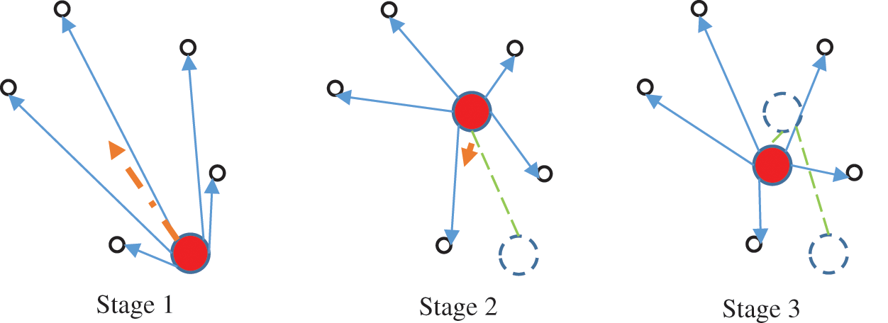
Figure 1: Three stages of GS algorithm execution in a data cluster

After executing the GS algorithm, the clustering must be evaluated based on the criteria to calculate the particle fitness (in the PSO algorithm). Appropriate evaluation criteria consider the distance between the data in the cluster and the cluster center and between the two clusters. Since the proposed method aims to find the minimum, we must invert the evaluation criteria, the higher values of which indicate better clustering quality. A simple solution adopted in this paper is multiplying the evaluation criterion result by −1 to demonstrate particle fitness. After evaluation, the velocity of each particle is achieved by using the PSO algorithm updating equation:

Vdj(t+1)=γVdj(t)+c1r1i[pbestdj−xdj(t)]+c2r2i[gbestdj−xdj(t)](37)

where pbest is the best position the particle has occupied, gbest is the best position of the particle in the population and v shows the particle’s velocity. By using the particle velocity, its position in the next iteration is specified:

xdj(t+1)=Vdj(t+1)+xdj(t)(38)

After finding the new position of each particle, the next round of the algorithm is executed.

2.10.1 Particle Structure

Particles are designed such that the number of clusters can also be obtained. Each particle has two parts. In the first part (selector), each element indicates whether the center of the corresponding cluster will appear as a cluster in the solution. For instance, the particle shown in Fig. 2 tries to cluster a dataset with dimensions of 3.

Figure 2: An example of particle structure in the proposed algorithm

In this example, if the value of each selector element is >0.5, the center of the corresponding cluster will be involved in clustering; otherwise, that cluster center will not be used. In this example, 0 particles cluster the data into three clusters. A piece of data may not belong to any cluster center; in this case, when using the GS algorithm, these cluster centers are removed to improve cluster centers. This is simply done by setting the value of the cluster selector to 0.

2.10.2 The Proposed Algorithm

A combination or hybridization involves combining two or more different things, which results in better results than their individual states. The GA and PSO algorithms have similar properties. Both have an initial random population and a certain amount of competency to assess the population. Therefore, combining these two methods can create an efficient hybrid algorithm.

In this section, we introduce the structure of the combined gravitational search algorithm and particle community. Fig. 3 shows a view of this algorithm.

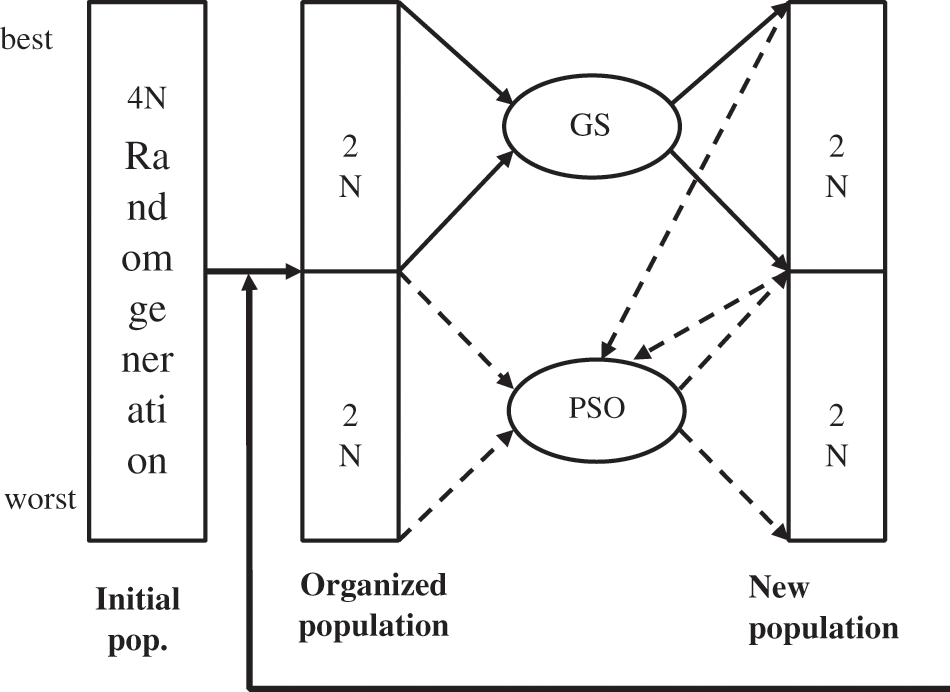
Figure 3: Combination of gravitational search algorithm () and particle swarm optimization ()

Fig. 3 shows that the combined gravitational search and particle clustering algorithm starts with an initial population. When the problem is next N, the hybrid algorithm is a 4N member that is generated completely randomly. 4N members are sorted by merit, 2N top members respond to the gravitational search algorithm, and a new 2N member population is created by mutation, generational intersection, and elitism. The lower member 2N is applied as a particle, a particle community optimization mechanism. In applying the particle optimization mechanism, the new population created by the gravitational search algorithm is used as the regulator. The best member of this new population is used as Pgbest, and each corresponding member is used as a neighborhood or Pibest in relation (37). The population resulting from the application of the particle optimization mechanism is merged with the population created by the gravitational search algorithm, the new 4N members are sorted according to merit, and the previous process is repeated until convergence is achieved. A combination of hybridization involves combining two or more different things, which results in better results than their individual states. The GA and PSO algorithms have similar properties. Both have an initial random population and a certain amount of competency to assess the population. Therefore, combining these two methods can create an efficient hybrid algorithm.

In this section, we introduce the structure of the combined gravitational search algorithm and particle community. Fig. 3 shows a view of this algorithm.

Fig. 3 shows that the combined gravitational search and particle clustering algorithm starts with an initial population. When the problem is next N, the hybrid algorithm is a 4N member that is generated completely randomly. 4N members are sorted by merit, 2N top members respond to the gravitational search algorithm, and a new 2N member population is created by mutation, generational intersection, and elitism. The lower member 2N is applied as a particle, a particle community optimization mechanism. In applying the particle optimization mechanism, the new population created by the gravitational search algorithm is used as the regulator. The best member of this new population is used as Pgbest, and each corresponding member is used as a neighborhood or Pibest in relation (37). The population resulting from the application of the particle optimization mechanism is merged with the population created by the gravitational search algorithm, the new 4N members are sorted according to merit, and the previous process is repeated until convergence is achieved.

The algorithm has the following steps:

1.    The initial population is randomly generated.

2.    The cluster centers are extracted in each particle.

3.    Data clustering is performed such that each piece of data belongs to a cluster center.

4.    The force applied to each cluster center is calculated based on the distance between the data of that cluster and the cluster center.

5.    The cluster center is displaced based on Equation 0.

6.    Go to Step 4 if there is any change in the cluster center.

7.    Updated centers’ coordinates are placed in the particle.

8.    Fitness is calculated based on an internal criterion.

9.    Gbest of all the particles and Pbest for each particle are selected.

10.   The position of each particle is updated based on Eqs. (36) and (37).

11.   Go to Step 2 if none of the exit conditions is met.

12.   Extract the cluster centers’ coordinates from the best particle and take them to the output as the clusters’ centers.

3  Test and Results

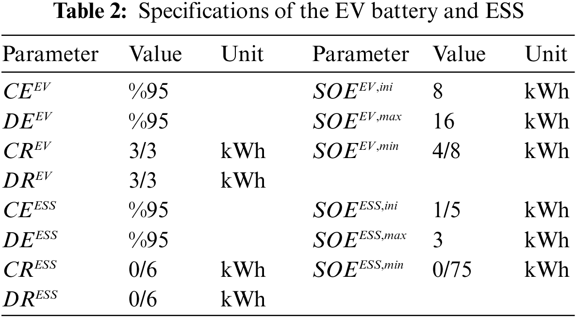
To evaluate the overall effects of different appliances on the consumer’s electricity bill, the proposed model for HEM is simulated in MATLAB and the results are discussed here. The data of STOU loads and non-shiftable appliances are presented in Table 1. The hourly demand curve of the non-shiftable TOU appliances and the curve of the solar power generated by a 500 W solar panel installed on the roof are given in Fig. 4 [32]. The technical and behavioral parameters of EV and ESS are presented in Table 2.

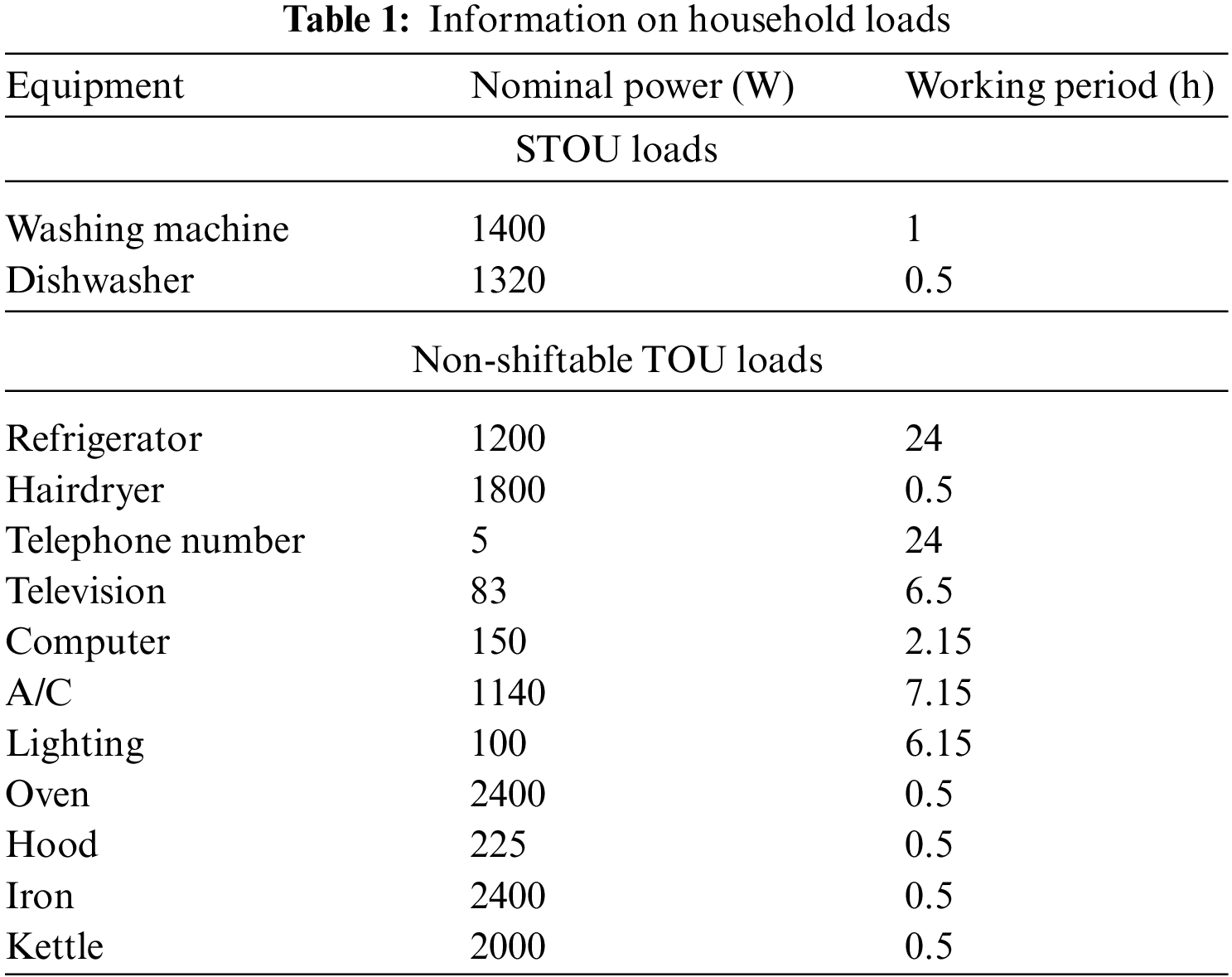
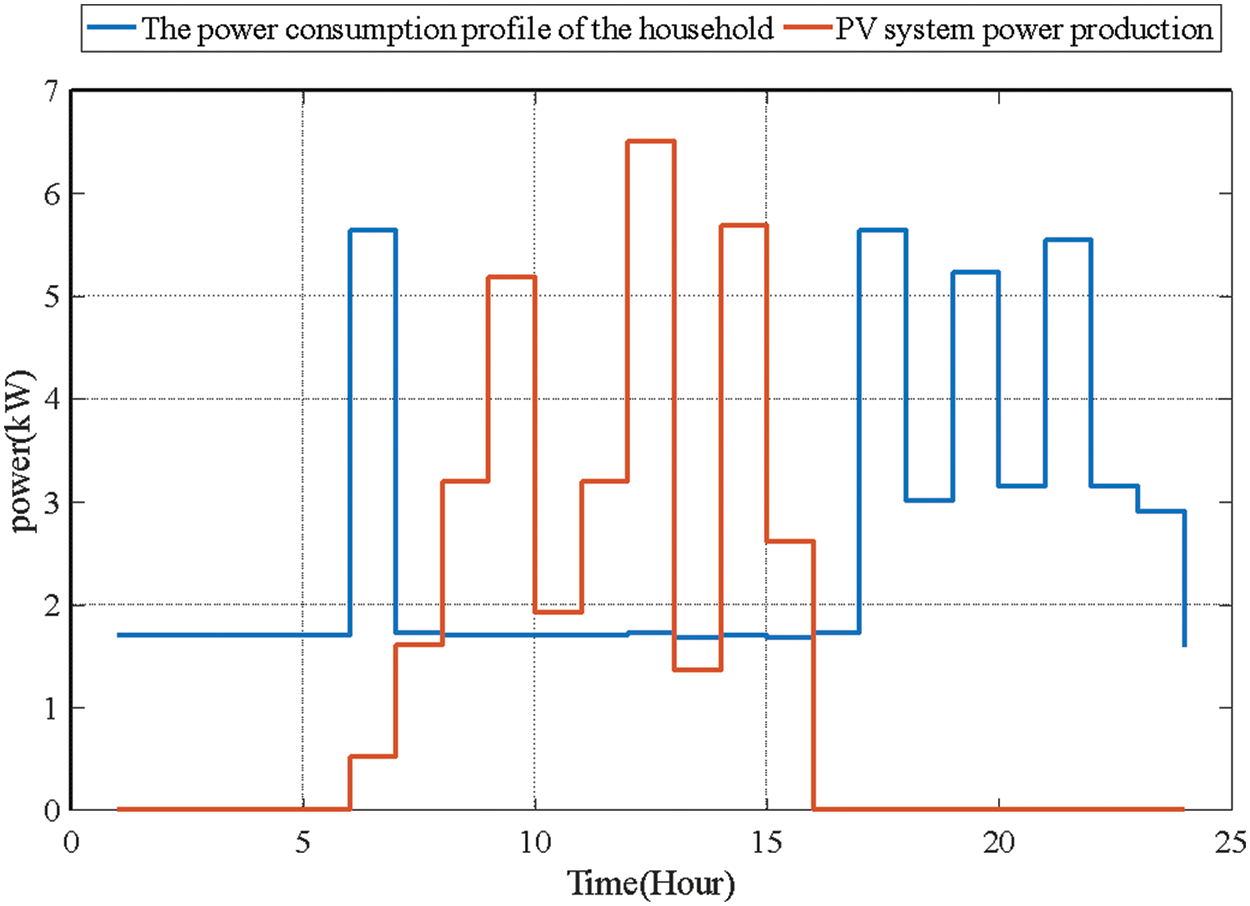
Figure 4: Load demand and solar power

It is assumed that the EV exits the parking lot at 7 a.m. and returns at 6 p.m. When the EV is leaving the parking lot, its battery must be charged to maximum capacity to prepare the EV for the trip. The distribution company determines the electricity purchasing price from the upstream grid. This price can be defined as different values in time blocks. Herein, the energy purchasing price is assumed hourly and based on Fig. 5. The energy sales price when injected into the grid, the energy sales price is assumed to be constant and equal to 4 cents/kWh [13].

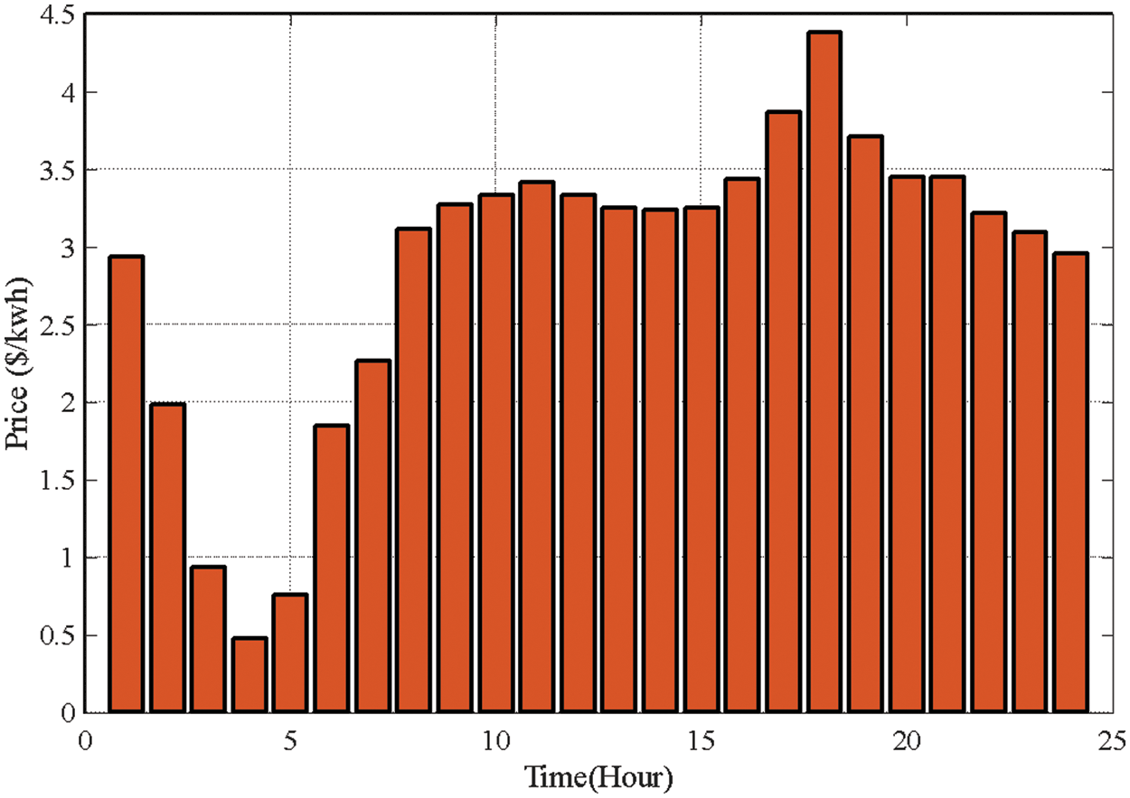
Figure 5: Energy purchasing price from the grid [4]

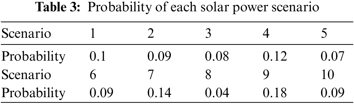
To predict the solar power, 100 scenarios were generated and then reduced to 10 to increase the computational speed and reduce the computation time. The scenarios for solar power prediction and the occurrence probability of each are presented in Table 3. To generate the scenarios of solar power, the SD is assumed to be 20% of the predicted value per hour.

3.1 Different States of Smart House Operation

Four states are assumed to evaluate the economic effects of using the equipment in the smart building. In all four states, the DR strategy is based on price, and the EV is in the parking lot from 6 p.m. to 7 a.m. the next day.

The first state: PV systems and ESS are not used.

The second state: A PV system with a generation power capacity of 500 W is used. It can sell the generated energy to the upstream grid and consume it for household uses.

The third state: In addition to the EV and PV system, an ESS with the capacity of 3 kWh is included.

The fourth state: By considering the uncertainty in solar power prediction, the smart house programming problem is stochastically programmed. In this state, by considering the CVAR, the values of α and β are assumed to be 0.8 and 0.2, respectively.

3.2 Results of the Proposed Model for Smart House Management

In the first state (DR program and EV included in the HEMS), the power exchanged with the grid is displayed in Fig. 6.

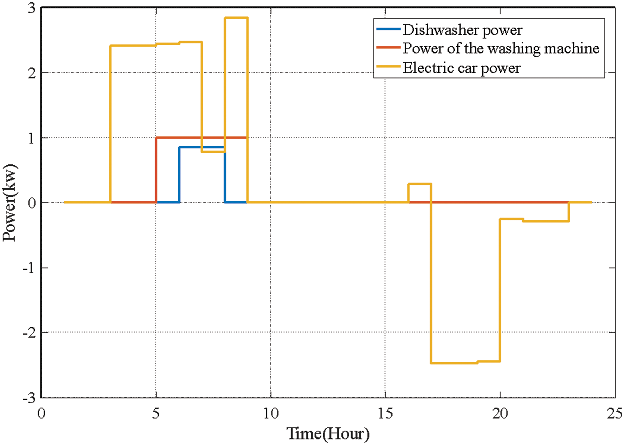
Figure 6: The power exchanged with the gird in the first state

The EV charge/discharge performance and the STOU loads are given in Fig. 7.

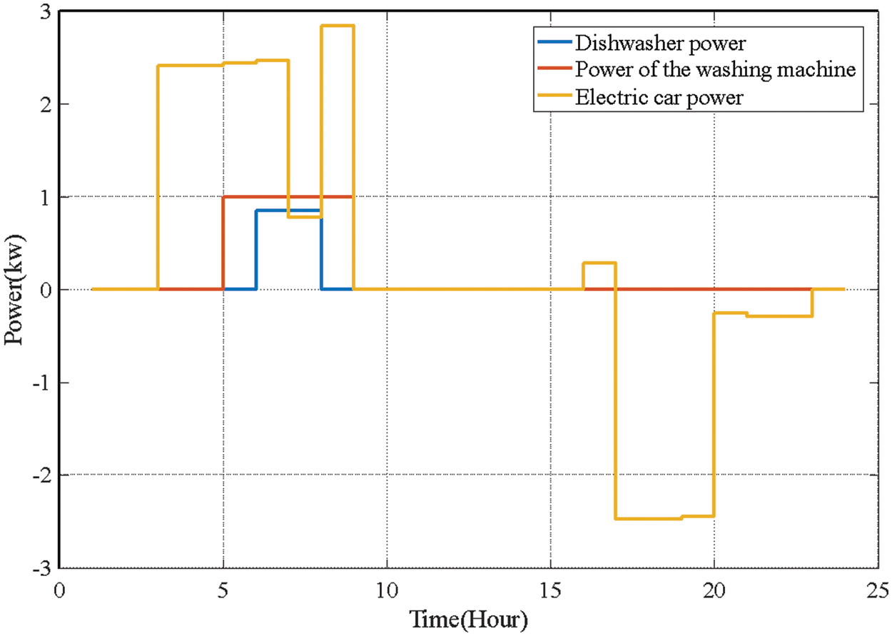
Figure 7: EV power and STOU loads in the first state

Based on Fig. 7, the difference between the consumed power of appliances with a determined TOU and the power received from the grid is due to the presence of EV and STOU loads. When the energy purchasing price is minimum, the EV is charged to the maximum, and the washing machine and dishwasher are turned on. When the price is maximum, the EV is discharged to the minimum and delivers its energy to the house. According to Fig. 8, the positive values indicate EV charging, and negative values indicate EV discharging.

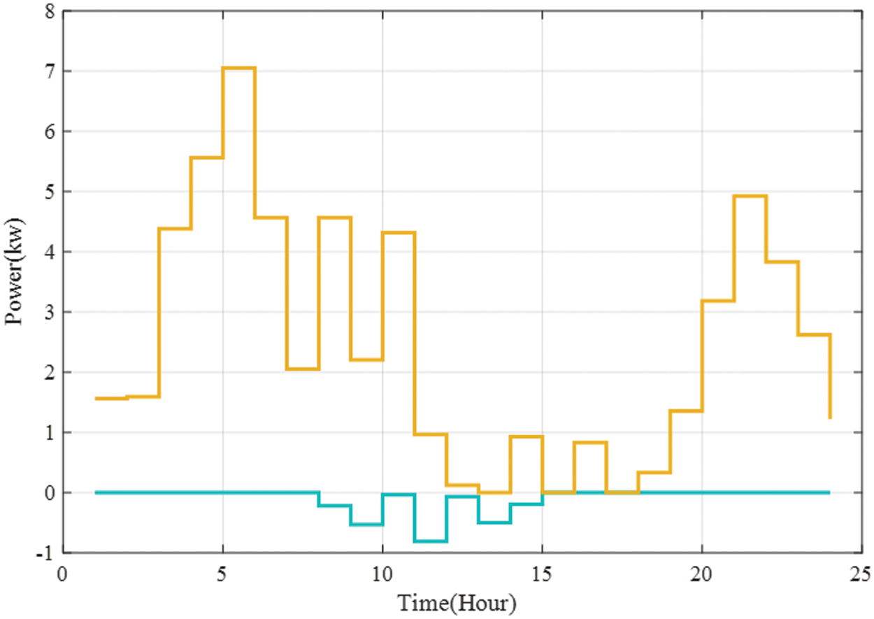
Figure 8: The power exchanged with the gird in the second state

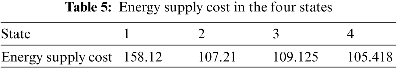
The energy supply cost is 157.58 cents in the first state. In the second state (PV system with 3 kWh capacity installed on the roof), variations in exchanged power with the grid are displayed in Fig. 8.

In Fig. 8, positive values of exchanged power indicate receiving power from the grid. In contrast, negative values indicate selling power to the grid. The power sold to the grid is the surplus of the power generated by the PV system. When the energy from the PV system is available, all the power consumed by the house is supplied, and no power is received from the grid.

In this case, the EV charge/discharge performance and the STOU loads are similar to the first state. When the energy price is minimum, the EV is charged to maximum; when the energy price is high, the EV is discharged as much as possible for internal use. The energy supply cost for the second state is 108.58 cents which are reduced compared to the first state due to using the PV system.

Results of the third state (EV, PV system, and ESS with 3 kWh capacity) are given in Figs. 9 and 10.

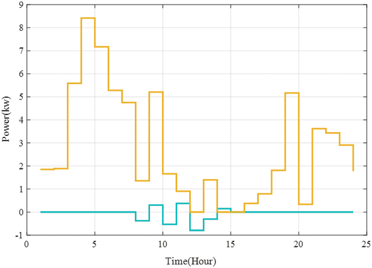
Figure 9: The power exchanged with the gird in the third state

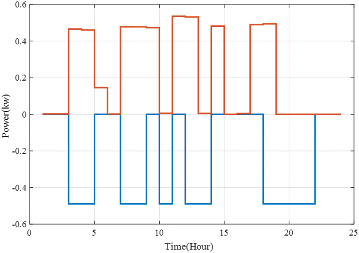
Figure 10: ESS power in the third state

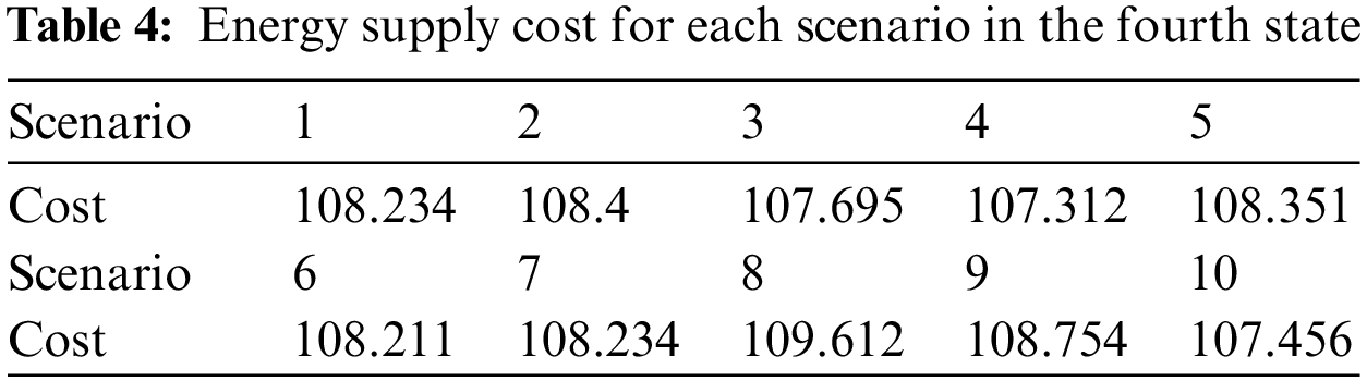
The power exchanged with the gird is displayed in Fig. 8, and the ESS charge/discharge performance is given in Fig. 10. In Fig. 8, the positive values indicate ESS SOC, and negative values indicate ESS SOD. The EV SOC and SOD results and shiftable appliances are similar to the first and second states. The energy supply cost for the third state is 108.212 cents which is reduced compared to the first state. In the fourth stage (PV system power modeled with uncertainty), the energy supply cost for each scenario is presented in Table 4.

The energy supply cost in the four stages is compared in Table 5.

The sensitivity of the expected cost of energy supply and the CVAR risk criterion to the beta parameter change for the fourth case, where the uncertainty in the prediction of solar power is considered, is shown in Fig. 11.

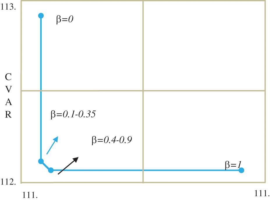
Figure 11: Sensitivity of the expected cost of energy supply and the CVAR risk based on beta change

According to Fig. 11, the expected cost of power supply and the CVART risk criterion are slightly sensitive to changes in the beta parameter. In this paper, only solar power is modeled as a random variable with uncertainty. Due to the capacity of solar panels, which has a relatively small share in smart home power supply and few options to decide on cost reduction in scenarios, there are differences There is, however, not much difference between the lowest and highest cost in the defined scenarios, which has led to the low sensitivity of the expected cost of energy supply and CVAR risk criterion to beta changes.

3.3 Proposed Algorithm Analysis

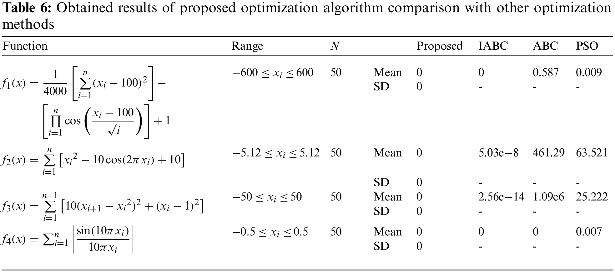
In this section, the proposed optimization algorithm is compared with other optimization methods. To cover the fair comparison condition, the benchmark function with the same parameters and area has been considered as presented in Table 6. Obtained results of the comparative analysis are presented in this table as well through the comparison with the artificial bee colony (ABC) algorithm, Improved ABC (IABC), and classic PSO. In all presented results, the proposed approach could outperform other optimization methods.

4  Conclusion

Most of the industrial and developing countries have recently paid attention to energy loss prevention in residential buildings. This issue has found more significance with the rising demands for oil and oil-generated energy. The need for new residential, administrative, educational, and other buildings, as well as the tendency to use the new equipment, have increased energy consumption in this sector. The global energy loss statistics show that wasteful energy consumption is higher in residential and commercial buildings than in other sectors. The current study proposed a model for home energy management to minimize the energy supply cost by considering STOU loads, EV with V2H capability, ESS, and PV systems. Due to the variable nature of RES, such as the PV system, uncertainty was considered in the formulation. Scenarios were generated by the LHS method and reduced by the backward method. A hybrid PSO and GS algorithm was used for optimization. The simulation results revealed that the energy supply cost could be reduced with the proper management of STOU appliances, and the grid could be aided in peak hours. To evaluate the economic effects of each system in the HEM, four states were considered, and the TOU of each STOU appliance was determined. Comparing the results indicated that including each additional system reduced the house energy supply cost.

Funding Statement: The authors received no specific funding for this study.

Conflicts of Interest: The authors declare that they have no conflicts of interest to report regarding the present study.

References

1. Duan, M., Darvishan, A., Mohammaditab, R., Wakil, K., Abedinia, O. (2018). A novel hybrid prediction model for aggregated loads of buildings by considering the electric vehicles. Sustainable Cities and Society, 41, 205–219. DOI 10.1016/j.scs.2018.05.009. [Google Scholar] [CrossRef]
2. Mohammadi, M., Talebpour, F., Safaee, E., Ghadimi, N., Abedinia, O. (2018). Small-scale building load forecast based on hybrid forecast engine. Neural Processing Letters, 48(1), 329–351. DOI 10.1007/s11063-017-9723-2. [Google Scholar] [CrossRef]
3. Cao, W., Pan, X., Sobhani, B. (2021). Integrated demand response based on household and photovoltaic load and oscillations effects. International Journal of Hydrogen Energy, 46(79), 39523–39535. DOI 10.1016/j.ijhydene.2021.08.212. [Google Scholar] [CrossRef]
4. Erdinc, O. (2014). Economic impacts of small-scale own generating and storage units, and electric vehicles under different demand response strategies for smart households. Applied Energy, 126, 142–150. DOI 10.1016/j.apenergy.2014.04.010. [Google Scholar] [CrossRef]
5. Nurmanova, V., Bagheri, M., Abedinia, O., Sobhani, B., Ghadimi, N. et al. (2018, October). A synthetic forecast engine for wind power prediction. 2018 7th International Conference on Renewable Energy Research and Applications (ICRERA), pp. 732–737. Paris, France, IEEE. [Google Scholar]
6. Wu, Y., Mäki, A., Jokisalo, J., Kosonen, R., Kilpeläinen, S. et al. (2021). Demand response of district heating using model predictive control to prevent the draught risk of cold window in an office building. Journal of Building Engineering, 33, 101855. DOI 10.1016/j.jobe.2020.101855. [Google Scholar] [CrossRef]
7. Babaei, M., Abazari, A., Soleymani, M. M., Ghafouri, M., Muyeen, S. M. et al. (2021). A data-mining based optimal demand response program for smart home with energy storages and electric vehicles. Journal of Energy Storage, 36, 102407. DOI 10.1016/j.est.2021.102407. [Google Scholar] [CrossRef]
8. Azimi, Z., Hooshmand, R. A., Soleymani, S. (2021). Optimal integration of demand response programs and electric vehicles in coordinated energy management of industrial virtual power plants. Journal of Energy Storage, 41, 102951. DOI 10.1016/j.est.2021.102951. [Google Scholar] [CrossRef]
9. Li, X. H., Hong, S. H. (2014). User-expected price-based demand response algorithm for a home-to-grid system. Energy, 64, 437–449. DOI 10.1016/j.energy.2013.11.049. [Google Scholar] [CrossRef]
10. Amer, A., Shaban, K., Gaouda, A., Massoud, A. (2021). Home energy management system embedded with a multi-objective demand response optimization model to benefit customers and operators. Energies, 14(2), 257. DOI 10.3390/en14020257. [Google Scholar] [CrossRef]
11. Judge, M. A., Manzoor, A., Maple, C., Rodrigues, J. J., ul Islam, S. (2021). Price-based demand response for household load management with interval uncertainty. Energy Reports, 8493–8504. DOI 10.1016/j.egyr.2021.02.064. [Google Scholar] [CrossRef]
12. Chen, X., Wei, T., Hu, S. (2013). Uncertainty-aware household appliance scheduling considering dynamic electricity pricing in smart home. IEEE Transactions on Smart Grid, 4(2), 932–941. DOI 10.1109/TSG.2012.2226065. [Google Scholar] [CrossRef]
13. Alizadeh, M., Jaafari, M. (2019). Smart home optimized energy management considering energy storage, solar cell, electric vehicle and load response. Journal of Modeling in Engineering, 17(57), 215–226. [Google Scholar]
14. Mohsenian-Rad, A. H., Leon-Garcia, A. (2010). Optimal residential load control with price prediction in real-time electricity pricing environments. IEEE Transactions on Smart Grid, 1(2), 120–133. DOI 10.1109/TSG.2010.2055903. [Google Scholar] [CrossRef]
15. Zhu, Z., Tang, J., Lambotharan, S., Chin, W. H., Fan, Z. (2012). An integer linear programming based optimization for home demand-side management in smart grid. 2012 IEEE PES Innovative Smart Grid Technologies (ISGT), pp. 1–5. Washington DC, USA, IEEE. [Google Scholar]
16. Hemmati, R., Saboori, H. (2017). Stochastic optimal battery storage sizing and scheduling in home energy management systems equipped with solar photovoltaic panels. Energy and Buildings, 152, 290–300. DOI 10.1016/j.enbuild.2017.07.043. [Google Scholar] [CrossRef]
17. Setlhaolo, D., Xia, X., Zhang, J. (2014). Optimal scheduling of household appliances for demand response. Electric Power Systems Research, 116, 24–28. DOI 10.1016/j.epsr.2014.04.012. [Google Scholar] [CrossRef]
18. Pipattanasomporn, M., Kuzlu, M., Rahman, S. (2012). An algorithm for intelligent home energy management and demand response analysis. IEEE Transactions on Smart Grid, 3(4), 2166–2173. DOI 10.1109/TSG.2012.2201182. [Google Scholar] [CrossRef]
19. Zamanloo, S., Abyaneh, H. A., Nafisi, H., Azizi, M. (2021). Optimal two-level active and reactive energy management of residential appliances in smart homes. Sustainable Cities and Society, 71, 102972. DOI 10.1016/j.scs.2021.102972. [Google Scholar] [CrossRef]
20. Molla, T. (2022). Smart home energy management system. In: Research anthology on smart grid and microgrid development, pp. 1132–1147. IGI Global. [Google Scholar]
21. Saeedirad, M., Rokrok, E., Joorabian, M. (2022). A smart discrete charging method for optimum electric vehicles integration in the distribution system in presence of demand response program. Journal of Energy Storage, 47, 103577. DOI 10.1016/j.est.2021.103577. [Google Scholar] [CrossRef]
22. ur Rehman, U., Yaqoob, K., Khan, M. A. (2022). Optimal power management framework for smart homes using electric vehicles and energy storage. International Journal of Electrical Power & Energy Systems, 134, 107358. DOI 10.1016/j.ijepes.2021.107358. [Google Scholar] [CrossRef]
23. Görgülü, H., Topçuoğlu, Y., Yaldız, A., Gökçek, T., Ateş, Y. et al. (2022). Peer-to-peer energy trading among smart homes considering responsive demand and interactive visual interface for monitoring. Sustainable Energy, Grids and Networks, 29, 100584. [Google Scholar]
24. Peng, P., Li, X., Shen, Z. (2022). Energy storage capacity optimization of residential buildings considering consumer purchase intention: A mutually beneficial way. Journal of Energy Storage, 51, 104455. DOI 10.1016/j.est.2022.104455. [Google Scholar] [CrossRef]
25. Li, R., SaeidNahaei, S. (2022). Optimal operation of energy hubs integrated with electric vehicles, load management, combined heat and power unit and renewable energy sources. Journal of Energy Storage, 48, 103822. DOI 10.1016/j.est.2021.103822. [Google Scholar] [CrossRef]
26. Rezaee Jordehi, A. (2021). An improved particle swarm optimisation for unit commitment in microgrids with battery energy storage systems considering battery degradation and uncertainties. International Journal of Energy Research, 45(1), 727–744. DOI 10.1002/er.5867. [Google Scholar] [CrossRef]
27. Ma, Y., Li, C., Zhou, J., Zhang, Y. (2020). Comprehensive stochastic optimal scheduling in residential micro energy grid considering pumped-storage unit and demand response. Journal of Energy Storage, 32, 101968. DOI 10.1016/j.est.2020.101968. [Google Scholar] [CrossRef]
28. Niknam, T., Azizipanah-Abarghooee, R., Narimani, M. R. (2012). An efficient scenario-based stochastic programming framework for multi-objective optimal micro-grid operation. Applied Energy, 99, 455–470. DOI 10.1016/j.apenergy.2012.04.017. [Google Scholar] [CrossRef]
29. Jordehi, A. R. (2019). Optimisation of demand response in electric power systems, A review. Renewable and Sustainable Energy Reviews, 103, 308–319. DOI 10.1016/j.rser.2018.12.054. [Google Scholar] [CrossRef]
30. Nojavan, S., Qesmati, H., Zare, K., Seyyedi, H. (2014). Large consumer electricity acquisition considering time-of-use rates demand response programs. Arabian Journal for Science and Engineering, 39(12), 8913–8923. DOI 10.1007/s13369-014-1430-y. [Google Scholar] [CrossRef]
31. Ailong, M. A., Zhong, Y., Zhang, L. (2014). Remote sensing imagery clustering using an adaptive bi-objective memetic method. 2014 IEEE Congress on Evolutionary Computation (CEC), pp. 50–57. Beijing, China, IEEE. [Google Scholar]
32. Umetani, S., Fukushima, Y., Morita, H. (2017). A linear programming based heuristic algorithm for charge and discharge scheduling of electric vehicles in a building energy management system. Omega, 67, 115–122. DOI 10.1016/j.omega.2016.04.005. [Google Scholar] [CrossRef]
Cite This Article
Copyright © 2022 The Author(s). Published by Tech Science Press.
This work is licensed under a Creative Commons Attribution 4.0 International License , which permits unrestricted use, distribution, and reproduction in any medium, provided the original work is properly cited.
Downloads
Citation Tools