Low-Carbon Dispatch of an Integrated Energy System Considering Confidence Intervals for Renewable Energy Generation

1  Introduction

Under the guidance of the dual-carbon target, the modern energy system is gradually transforming into a new energy system with renewable energy as the main source. Within this emerging energy framework, Integrated Energy Systems (IES) with electric-thermal coupling as the core enhances low-carbon energy utilization through multi-source coupling conversion, which provides an effective way to promote low-carbon emission reduction and improve energy utilization efficiency in the energy transition process [1].

The distributed generation (DG) within IES is gradually transitioning to become the predominant energy source for the energy system due to its zero-carbon characteristics [2,3]. However, the randomness and predictive errors associated with DG necessitate that IES possess substantial peak-shaving capabilities. During the energy dispatch process, it is imperative to prepare for peak-shaving reserves to mitigate the risk of insufficient downward reserves within the IES. This inadequacy could otherwise lead to instances of curtailed solar and wind power and limitations on carbon emissions reduction potential. Therefore, it is critical to optimize the control functions within the multi-source coupling elements of the IES. Achieving a harmonious balance between ensuring the low-carbon operation of the IES and utilizing the regulation capabilities in generation, demand and storage becomes essential. This pragmatic approach not only helps to align with the salient features of renewable energy generation but also helps to develop economically viable dispatch strategies. Consequently, it holds pivotal significance in realizing the objective of achieving low-carbon operations within the modern landscape of integrated energy systems.

Since IES carbon emissions mainly originate from coal and other energy sources consumed by power-side generating units for energy supply [4], source-side cogeneration units utilizing carbon capture and sequestration technology for carbon capture retrofit can become an ideal complementary power source for renewable energy power generation. Currently, carbon capture power plants primarily employ two methods for carbon capture: the shunt type and the liquid storage type. Among them, the shunt type carbon capture power plant carbon capture energy consumption and unit power are positively correlated [5], and CO2 must be continuously captured and analyzed. Liquid storage carbon capture power plants exhibit ``energy time-shift characteristics'' [6], allowing for the timely storage of captured CO2. However, economic conflicts may arise when carbon trading prices are low. The emergence of integrated and flexible operations in carbon capture plants, which combine both shunt and liquid storage methods [7,8], addresses the limitations of individual approaches and achieves the separation of CO2 absorption and capture processes. Furthermore, determining how to effectively employ carbon capture operational adjustments to broaden the output spectrum of carbon capture power plants, thereby enhancing the source-side carbon capture power plant's capability for energy time-shift adjustments to accommodate fluctuations in renewable energy power generation, holds substantial significance in mitigating carbon emissions within the IES.

Differing from source-side carbon capture power plants that directly capture and absorb CO2, the load and storage side within IES adjusts its operational conditions through demand response and grid regulation. This response aims to address fluctuations in distributed generation (DG) power output, indirectly contributing to the reduction of the system's carbon emissions. Notably, research regarding the involvement of electric/thermal energy storage systems (ESS) in regulation applications has been progressively expanding. It has evolved from focusing solely on single-system optimization [9] to encompassing optimization across diverse scenarios within the IES framework [10]. Additionally, load-side controllable loads have initiated participation in the optimization of IES operations through demand response mechanisms [11,12]. Reference [13] delved into the influential role of existing carbon trading mechanisms on IES operations, while reference [14] proposed a heuristic algorithm-based approach for load scheduling and energy storage system management. Nevertheless, the existing coordination and optimization strategies for resources on the load and storage side within the IES predominantly rely on deterministic wind and solar forecasts [15]. Unfortunately, this approach tends to overlook discrepancies between actual values and predictions due to the inherent variability of wind and solar resources. This oversight results in inadequate consideration of the available margins for various resource types.

The objective of this article is to delve into the backdrop of multi-source coupling within IES, the integrated flexible operational mode of source-side carbon capture power plants in IES, and the extent to which the coordination attributes of the flexibility of resources on the load and storage side have been comprehensively considered, as this has a bearing on the holistic realization of low-carbon complementary advantages. Moreover, the passive consumption scenario resulting from the volatility and unpredictability of renewable energy sources, such as wind and solar, demands assurance that the predictive errors associated with distributed generation within IES possess the requisite coping capacity at the day-ahead stage.

The main contributions of this work can be summarized as follows:

(1) This study centres on the regional IES as its focal research target. The analysis investigates the energy time-shift characteristics intrinsic to the integrated flexible operation of the source-side carbon capture power plant. Simultaneously, it evaluates the regulatory attributes and carbon-reduction adaptability exhibited by the flexible resources on the load and storage components. Leveraging the low-carbon synergies inherent in IES source-load-storage resources, this research introduces a coordinating low-carbon scheduling mechanism. This mechanism ensures seamless coordination among the source, load, and storage aspects.

(2) Given the varying confidence intervals associated with wind and solar renewable energy sources, along with the downward adjustment margin reserve of flexibility resources, and taking into account the dispatchable resource utilization efficiency, an IES day-ahead dispatch model is formulated. This model incorporates confidence intervals, effectively bolstering the IES's capacity to accommodate errors in renewable energy forecasts.

(3) Taking the electric-thermal coupling system as an example, the comprehensive benefits of IES are evaluated through simulation, and the coordinated operation of the source-load-storage side under different scenarios is analyzed, which effectively reduces the carbon emission of the system after optimization, improves the economic benefits of the system operation, and provides auxiliary guidance for the optimized operation of IES in a low-carbon environment.

2  Analysis and Modeling of the Source-Load-Storage Mechanism of IES

Electric-thermal coupled IES is powered on the supply side by carbon capture power plants, conventional cogeneration units, higher-level grids, as well as wind and photovoltaic power sources. On the demand side, the user's production process undergoes adjustments via demand response mechanisms, effectively addressing the requirements for IES peak shaving and valley filling. Concurrently, the storage facet is managed through the synergy of electric and thermal energy storage. Notably, the IES's internal electric and thermal network is intricately linked with electric heating equipment via cogeneration units, thereby enabling seamless energy conversion. This synergy facilitates the dynamic bidirectional energy flow, underscoring the exploration of synergistic potentials among the supply, demand, and storage components.

In response to the diversified needs of users within the IES, an integrated electric-thermal energy system, as shown in Fig. 1, is established to safeguard electric and thermal load demand.

Figure 1: The structure of IES

2.1 Mechanistic Analysis and Modelling of Carbon Capture Power Plants

The integrated flexible operation of carbon capture power plants consists of two parts: split-flow and liquid storage operation [16]. The split-flow operation controls CO2 emissions by adjusting the flue gas bypass, while the liquid storage operation decouples the CO2 capture and absorption processes by relying on liquid storage equipment, allowing the unit to adjust the power consumption for CO2 capture and absorption at any time. The integrated flexible operation mode combines the advantages of the two operation modes, converting the CO2 that should be captured in real-time during peak load periods into storage in solution to reduce direct carbon emissions, and consuming the pre-stored CO2 in solution during low load periods to make full use of the unit's residual power while reducing the unit's carbon emissions. Through the process of storing and recapturing the carbon emissions of the unit, the flexible transfer of CO2 is finally realized, which enables the unit to meet the demand for energy supply during the peak load period and fully utilize the remaining power of the unit during the low load period, which is beneficial to the auxiliary IES for renewable energy consumption.

After the installation of carbon capture devices in ordinary CHP, the total output of the carbon capture unit is increased by the carbon capture energy power on top of the net output of the unit. The carbon capture energy power is composed of fixed energy consumption and operating energy consumption [17], and the operating energy consumption is composed of resolved energy consumption and compression energy consumption [18]. The carbon capture power plant model is thus established, as shown in Eq. (1) [19].

{ PGi,t=PJi,t+σGϕGi,t+PDi+PBi,tEtotalCO2i,t=ESGi,t+βδiEGi,t0≤EtotalCO2i,t≤ηβegiPGi,maxPBi,t=λEtotalCO2i,tEGi,t=egiPGi,t(1)

In the above equation, PGi,t, PBi,t, PJi,t, PDi,t are the total output power, operating energy consumption, net output power, and fixed energy consumption of unit i at time t, respectively; EGi,t, EtotalCO2i,t, ESGi,t are the total amount of CO2 produced by unit i at time t, the total amount of CO2 already captured, and the amount of CO2 provided by the solution memory, respectively; egi is the carbon emission intensity of unit i; σG is the reduction value of output electric power when extracting unit steam volume at the fixed steam inlet; δi is the flue gas split ratio of unit i; β is the carbon capture efficiency; η is the maximum operating condition factor of regeneration tower and compressor; λ is the energy consumption for capturing unit CO2.

From the derivation of Eq. (1), the expression of the net output range of the carbon capture unit is shown in Eq. (2) [19].

PGi,min−ληβδmaxeg,iPGmax−PD,i≤PJt,i≤PGi,max−PD,i(2)

Observably, when considering equivalent installed capacities, the carbon capture plant exhibits a heightened capacity for carbon capture in comparison to a conventional CHP unit devoid of carbon capture technology. This discrepancy leads to a diminished net output threshold. Additionally, the incorporation of a solution memory configuration assigns a modifiable power allocation to the unit, yielding an energy-time-shifting phenomenon. This temporal energy adjustment serves to further curtail the unit's lower net output boundary, thereby enhancing its alignment with the requisites of renewable energy generation and bolstering its efficacy in responding adeptly to low-carbon imperatives.

2.2 Modeling of Controllable Loads

The load-side controllable load has the characteristics of large scale and obvious influence by the user's type of electricity consumption, which is regulated directly by the superior grid or its initiative to respond to the change of electricity price, change the user's production process, adjust the working hours to shift and cut its electricity consumption in response to the IES regulation demand. According to the characteristics of controllable load, the electrical load is divided into two categories: transferable load and interruptible load [20]. The controllable loads are modelled as follows:

PDR,t=PL,t+PTSL,t−PIL,t(3)

In the above equation: PDR,t, PL,t are the post and pre-electric load values of the electric load demand response at time t; PTSL,t is the transferable electric load value; PIL,t is the interruptible electric load at time t.

Transferable load maintains the same total load throughout the dispatch cycle by reallocating part of the load from the original consumption period. It satisfies the following constraints:

PTSL,t,min≤|PTSL,t|≤PTSL,t,max(4)

∑t=124PTSL,t=0(5)

In the above equations: PTSL,t,max, PTSL,t,min are the upper and lower limits of transferable electric load at time t, respectively.

The interruptible load is part of the load that is cut in response to the power system’s peak demand during the tight power supply time, and the pressure of supplying energy on the IES source side is relieved by economic subsidies. It satisfies the following constraints:

0≤∑t=124PIL,t≤PIL,max(6)

In the above equation: PIL,t,max is the maximum total interruptible load.

2.3 Modeling of Electric Heating Equipment

Electric heat production equipment is generally based on high-grade heat production equipment such as electric boilers, which effectively connect the IES electric heat coupling link and can quickly and efficiently convert excess electricity that cannot be consumed by the power system during the time of large differences in electric heat demand, providing another effective channel for low-carbon emission electric energy consumption during the low load period, while relieving the heat supply pressure of CHP units. The model is:

ϕEB,t=εEBPEB,t(7)

0≤PEB,t≤PEB,max(8)

In the above equations: ΦEB,t is the heating power of electric heating equipment; PEB,t is the electric power consumed by electric heating equipment; PEB,max is the maximum power of electric heating equipment; εEB is the electric heat conversion efficiency.

2.4 Modeling of Energy Storage Devices

Electric/thermal energy storage in IES plays a flexible regulating role during operation, storing low-carbon clean energy that is difficult to consume by IES during large-scale renewable energy generation, and making timely supply during periods of high load demand to reduce IES carbon emission pressure and adapting to IES dynamic regulation needs.

The installation of Battery Energy Storage (BES) and Thermal Energy Storage (TES) can promote the reduction of carbon emission levels in electric-thermal systems. A unified model of the response characteristics and constraints of the two types of energy storage is shown below:

Ei,t=Ei,t−1+PESS,c,i,tμc−PESS,dis,i,t/μdis(9)

Emin≤Ei,t≤Emax(10)

δESS,c,tPESS,c,min≤PESS,c,t≤δESS,c,tPESS,c,max(11)

δESS,dis,tPESS,dis,min≤PESS,dis,t≤δESS,dis,tPESS,dis,max(12)

δESS,dis,t+δESS,c,t≤1(13)

In the above equations: Ei,t is the remaining capacity of the ith energy storage device in time t, Emax, Emin are the upper and lower limits of energy storage capacity; PESS,c,i,t, PESS,dis,i,t are the charging/supplying power of energy storage device i in time t, PESS,c,max, PESS,c,min, PESS,dis,max, PESS,dis,min are the upper and lower limits of the charging/supplying power of the energy storage device; μc, μdis are the charging/supplying efficiency of the energy storage; δESS,c,t, δESS,dis,t indicate the working state of the energy storage, with 0 representing the non-working state and 1 representing the working state.

3  IES Low Carbon Economic Dispatch Model Considering Confidence Intervals for Renewable Energy Generation

3.1 Choice of an Upper Limit of a Flexible Confidence Interval for Renewable Energy

Acknowledging the inherent unpredictability in forecasting scenic renewable energy outputs, an IES scheduling model predicated upon confidence intervals is introduced. This model adeptly addresses the oscillations within scenic renewable energy generation profiles, facilitating the optimized utilization of low-carbon renewable resources. Moreover, it ensures the equilibrium of electricity and heat outputs within the IES domain by orchestrating resource allocation intricacies intrinsic to the system’s internal dynamics.

Since the forecast curve and confidence interval of renewable energy generation can only be obtained in the day-ahead scheduling stage, this paper considers the scenario of wind and light abandonment due to insufficient IES down the regulation margin and plays the role of IES source-load-storage regulation to make down-regulation margin reserve in the scheduling stage to cope with the fluctuation of renewable energy generation output. The downward adjustment margin is composed of common CHP units, carbon capture units, electric heating production equipment, electric and thermal energy storage and controllable loads. While dispatching according to the scenic power forecast curve, a sufficient downward margin is provided for IES, and the downward margin constraints need to be satisfied during the dispatching process:

PEB,max−PEB,h,t+PESS,c,i,t−PESS,dis,i,t+PJi,t−PJi,min+PGi,t−PGi,min=PWup+PVup−PW−PV(14)

In the above equation, PWup, PVup are the upper confidence interval of wind power and photovoltaic power generation, and PW, PV are the predicted values of wind power and photovoltaic power generation.

Due to discernible disparities among the projected curves for renewable energy generation and the associated confidence intervals, the upper bound of the confidence interval is established by considering the variations across these intervals for both wind and photovoltaic outputs. For the sake of illustrative computations, confidence intervals ranging from 70% to 100% are determined in increments of 10% [21]. In line with reference [21], a 10% interval differential identifies the 90% interval as the most reliable prediction range, encapsulating a substantial portion of actual values. Consequently, the mean divergence between the upper limits of the confidence interval for renewable energy power generation at 100% and 70% throughout the prediction interval is adopted as a reference criterion. When a considerable deviation exists between the 100% confidence interval and the reference value, it indicates relatively diminished prediction accuracy during that timeframe. Accordingly, the upper limit of the 90% confidence interval is selected as the definitive upper bound for renewable energy power generation. This choice facilitates prudent provisioning for renewable energy consumption while avoiding unwarranted overestimation. Conversely, when deviations fall below the average threshold, indicative of heightened forecast precision for that period, resource scheduling adheres to the original projected curve to prevent unwarranted downward adjustments. This dynamic framework establishes a flexible upper limit for the confidence interval, enabling the IES to effectively address potential resource misallocation resulting from predictive errors. It allows for ample leeway in downward adjustments, simplifying dispatcher decisions for suitable renewable energy forecast intervals contingent upon real-world circumstances.

ΔPave,t=(P100up,tYU−P70up,tYU)/∑t=124(P100up,tYU−P70up,tYU)(15)

PtYC={P90up,tYU,(P100up,tYU−P70up,tYU)≥ΔPave,tPtYU,(P100up,tYU−P70up,tYU)<ΔPave,t(16)

In the above equations: P100up,tYU, P90up,tYU, P70up,tYU are the upper confidence interval of 100%/90%/70% renewable energy generation at time t, respectively, PYCt is the renewable energy forecast curve obtained after considering the difference of confidence intervals at time t, and ΔPave,t is the average value of the difference between 100% confidence interval and upper 70% confidence interval at time t.

3.2 Objective Function

In this paper, we construct a low-carbon dispatch model with IES-integrated cost optimization as the objective function.

minf=CG+Cq+Cy+Cz+CS+CDR+CESS+CTES+Cbuy(17)

In the above equation: f is the comprehensive cost of the dispatch model; CG is the cost of supplying thermal power units; Cq is the total cost of abandonment penalty; Cy is the cost of carbon trading; Cz is the cost of renovation and depreciation of carbon capture power plants; CS is the cost of solvent loss in the carbon capture process; CDR is the cost of demand-side response regulation; CESS, CTES are the cost of charging/supplying electric and thermal energy storage, respectively; Cbuy is the cost of purchasing power from the upper grid.

3.2.1 Cost of Supplying Energy to Thermal Power Units (CG)

CG=∑t=124∑i=1M[ai(PG,i,t+σGϕG,i,t)2+bi(PG,i,t+σGϕG,i,t)+ci](18)

In the above equation: ai, bi, ci are the coal consumption cost coefficients of unit i, respectively; M is the number of units.

3.2.2 Total Cost of Wind Abandonment Penalty (Cq)

Cq=∑t=124KqPwq,t(19)

In the above equation: Kq is the penalty cost per unit of abandoned wind volume; Pwq,t is the abandoned wind power at time t.

3.2.3 Cost of Carbon Trading (Cy)

Cy=Ky[Ec−∑i=1M∑t=124(δhPGi,t)](20)

In the above equation: Ky is the carbon trading price; Ec is the total carbon emission of the system; δh is the carbon emission allowance factor.

3.2.4 Daily Depreciation Cost of Carbon Capture Power Plant (Cz)

Cz=CFL(1+r)Nzlr365[(1+r)Nzl−1]+PRYVRY(1+r)NRYr365[(1+r)NRY−1](21)

In the above equation: r is the discount rate of the carbon capture plant; CFL and Nzl are the total cost of carbon capture equipment and depreciable life of the split-flow plant, respectively; PRY is the total cost of solution storage per unit volume of liquid storage carbon capture plant; VRY and NRY are the volume of solution storage and depreciable life, respectively.

3.2.5 Solvent Loss Cost (CS)

CS=∑t=124∑i=1MKSφEtotalCO2i,t(22)

In the above equation: KS is the ethanolamine solvent cost factor; φ is the solvent running loss factor.

3.2.6 Energy Storage Operating Costs (CESS, CTES)

CESS=βprice,iESS∑t=124(|PESS,c,i,t|+|PESS,dis,i,t|)(23)

CTES=βprice,iTES∑t=124(|ϕTES,c,i,t|+|ϕTES,dis,i,t|)(24)

In the above equations: ϕTES,c,i,t, ϕTES,dis,i,t are the charging/supplying power of thermal energy storage device i in time period t; βESSprice,i, βTESprice,i are the charging/supplying O&M costs of electric and thermal energy storage.

3.2.7 Cost of Load Regulation (CDR)

CDR=eprTSL∑t=124PTSL,t+eprIL∑t=124PIL,t(25)

In the above equation: eprTSL is the unit transferable load adjustment price; eprIL is the unit interruptible load adjustment price.

3.2.8 Cost of Power Purchase from the Upper Grid (Cbuy)

CBY=∑t=124eprice,tPBY,t(26)

In the above equation: eprice,t is the time-sharing tariff for electricity purchased from the upper grid in time period t.

3.3 Constraints

3.3.1 Constraint with the System’s Electrical Power Balance

∑i=1MPG,i+PW+PV+PESS,dis+PBY=PLOAD+Pwq+PEB+PDR+PESS,c(27)

3.3.2 Constraint on the Thermal Power Balance of the System

∑i=1MϕG,i+ϕEB+ϕTES,dis=ϕLOAD+ϕTES,c(28)

3.3.3 Climbing Constraints of Cogeneration Units

PG,t−PG,t−1≤ΔPu(29)

PG,t−1−PG,t≤ΔPd(30)

In the above equations: PG,max, PG,min are the maximum and minimum electric output of the CHP unit; ϕG,max, ϕG,min are the maximum and minimum heat output of the CHP unit; ΔPu, ΔPd are the climbing rate of the unit.

3.3.4 Constraints for Integrated Flexible Operation Mode Carbon Capture Power Plants

Carbon capture power plants are retrofitted based on ordinary CHP units with the same output constraint climbing constraint as conventional CHP units.

Considering the carbon capture power plant storage constraint, this paper refers to the treatment in reference [19] and expresses the CO2 mass in the form of solution volume, as shown in the following equation:

VCA,t=ESG,tMMEAMCO2θCRρR(31)

In the above equation: VCA,t is the volume of solution required to provide CO2 at time t from the solution memory installed in the power plant; MMEA and MCO2 are the molar masses of MEA and CO2; θ is the regeneration tower resolution; CR is the concentration of the alcohol amine solution; ρR is the density of the alcohol amine solution.

The solution memory constraint contains the reservoir volume constraint and the reservoir volume change constraint, as shown in the following equation [19]:

{ VCFYt=VCFYt−1−VCAtVCPYt=VCPYt−1−VCAt0≤VCFYt≤VCR0≤VCPYt≤VCRVCFY0=VCFY24VCPY0=VCPY24(32)

In the above equation: VFY,t and VPY,t are the solution volumes of the liquid-rich memory and the liquid-poor memory at time t, respectively; VCR is the capacity of the solution memory; VFY0, VPY0, VFY24, VPY24 are the solution volumes of the liquid-rich memory and the liquid-poor memory at the beginning/end of the scheduling cycle, respectively.

3.4 Low Carbon Economy Scheduling Model Solution Principles

The core solution principle of the developed IES low-carbon economic dispatch model, as presented in this study and taking into account the confidence intervals of renewable energy generation, is depicted in Fig. 2.

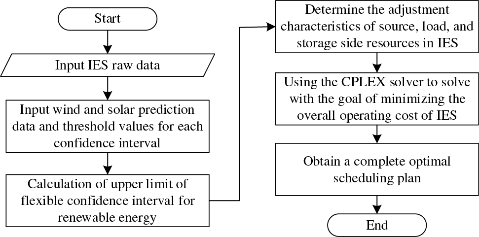
Figure 2: Low-carbon scheduling model solution principle

The fundamental approach presented in this paper entails establishing the parameters for each constituent component within the IES. This involves inputting the forecast data for wind and solar irradiation, subsequently delineating upper and lower bounds for the confidence intervals. Subsequently, calculations are performed to derive the upper limit of the adaptable confidence interval for renewable energy. Building upon these calculations, day-ahead optimization of scheduling is executed encompassing the source-side cogeneration units, carbon capture units, storage-side electric and thermal energy storage, and load-side controllable loads within the IES. The optimization process revolves around the objective of minimizing the integrated cost of the IES. In doing so, the achievable downward reserve margin within the IES under diverse scenarios is assessed, ultimately yielding an optimized scheduling plan. Furthermore, this approach facilitates an examination of the contribution of each system component within the scheduling outcome towards enhancing the low-carbon advantages inherent to the IES.

4  Example Analysis

To verify the effectiveness of the proposed scheduling model, a winter IES in a region of North China is used as an example for analysis.

4.1 Parameter Setting of the Algorithm

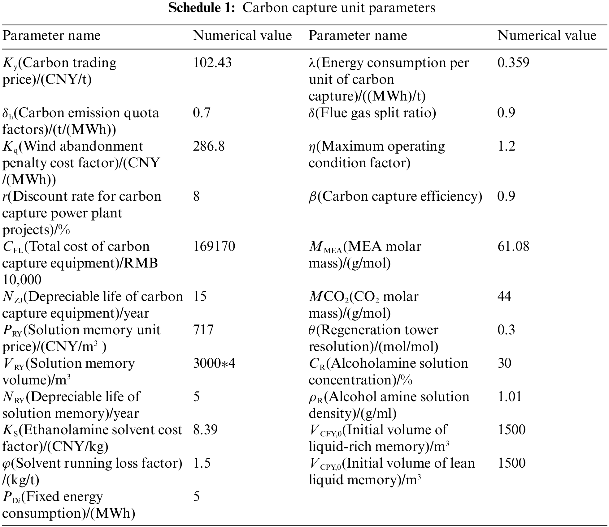
Two CHP units are installed in this regional IES, one unit is converted into a carbon capture power plant and the other unit is a normal CHP unit, the basic parameters of the two units are the same, and the detailed parameters are shown in Table 1, detailed parameters of the carbon capture unit are shown in schedule 1 in the Appendix A [22]. The maximum power of both transferable and interruptible electrical loads is set at 5% of the peak electrical load for each time, where the transferable load subsidy price is 0.26 RMB/kW and the interruptible load terminal adjustment price is 0.4 RMB/kW [23].

During the dispatch cycle, the electric and thermal load demand is shown in Fig. 3. The power purchase price of IES from the superior grid is shown in Fig. 4 [24]. The carbon intensity factor of the power purchase from the superior grid is set to 1. The electric/thermal energy storage parameters are shown in Table 2. The power limit of the electric heating equipment is 10,000 kW, and the efficiency of the heating is 0.95. The rest of the system parameters are shown in the attached Table 1. The simulation environment of this paper is Intel Core i5-9300H CPU, 16 GB RAM, compiled and tested in MATLAB R2020b using CPLEX.

Figure 3: Power/heat load demand curve

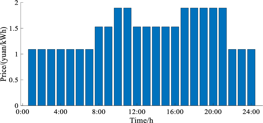
Figure 4: Time of use price

Based on the confidence interval distributions of wind power and PV provided in references [21,25], the results are shown in Figs. 5 and 6, respectively. The curves in Figs. 5 and 6 are 100%, 90%, 80%, and 70% confidence intervals from outside to inside, respectively, setting the installed capacity of scenic power for 30,000 kW.

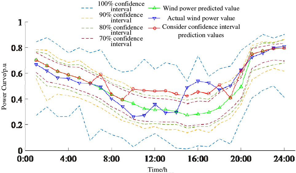
Figure 5: Confidence interval and prediction curve of wind power

Figure 6: PV confidence interval and prediction curve

From the analysis of Figs. 5 and 6, it is evident that there exist minimal discrepancies within the confidence intervals of PV power generation. Furthermore, the PV-predicted values exhibit a high degree of alignment with the actual PV values. Remarkably, throughout the entirety of the prediction period, the adaptable upper boundary of the PV power generation’s confidence interval closely aligns with the PV predicted values. Compared with PV, the difference between the confidence intervals of wind power is more obvious, especially in the period of 14:00–20:00, the predicted and actual values of wind power have produced significant differences, and the actual values have crossed the upper bound of the 90% confidence interval. This indicates that wind power has high uncertainty and low prediction accuracy, so if we rely on wind power prediction for pre-IES dispatch, it will lead to insufficient available regulation margin and a large amount of abandoned power when wind power generation is higher than the predicted value. Therefore, different scenarios are classified according to the reference upper limit of the downward adjustment margin of controllable resources in the IES day-ahead scheduling process.

(1) Scenario 1: Using wind power and PV actual forecast values for IES day-ahead dispatching, without considering the dispatching downward adjustment margin reserve, and obtaining IES source-load-storage optimal dispatching results;

(2) Scenario 2: Considering the forecast error due to scenery renewable energy, while dispatching according to the forecast value, the margin reserve is adjusted downward according to the upper limit of 70% scenery confidence interval, and the IES source load storage optimized dispatching result is obtained;

(3) Scenario 3: Considering the scenery renewable energy forecast error, while dispatching according to the forecast value, the margin reserve is adjusted downward according to the upper limit of the flexible confidence interval for renewable energy generation, and the IES source load storage optimized dispatch results are obtained.

4.2 Analysis of Algorithm Results

The scheduling cost results for each scenario are shown in Table 3, and the source load storage scheduling results are shown in Figs. 7–12.

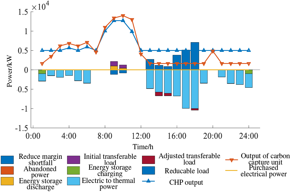
Figure 7: Scenario 1 power system results

Figure 8: Scenario 1 thermal system results

Figure 9: Scenario 2 power system results

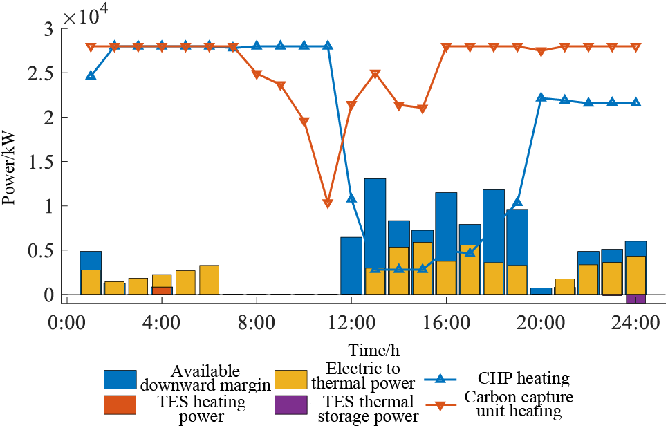
Figure 10: Scenario 2 thermal system results

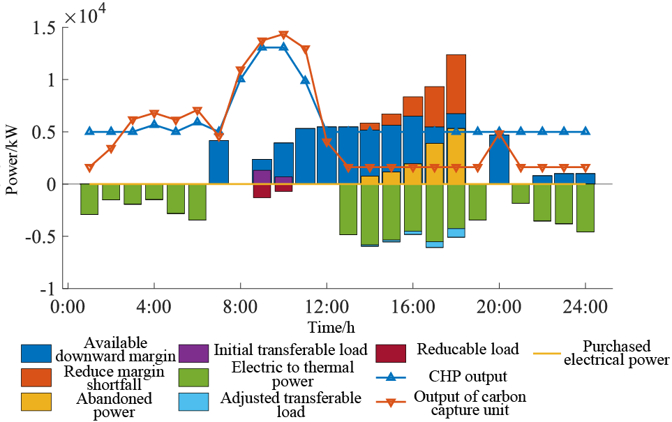
Figure 11: Scenario 3 power system results

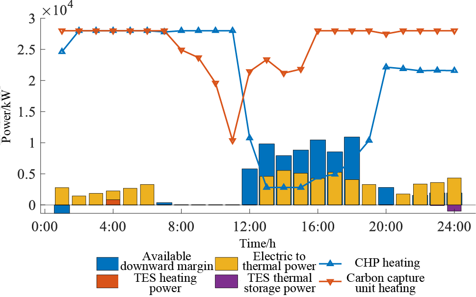
Figure 12: Scenario 3 thermal system results

Observing Figs. 7 and 8, it becomes apparent that in Scenario 1, when not factoring in the downward adjustment of margin reserves, scheduling based on the anticipated wind and photovoltaic power generation profiles facilitates the complete utilization of renewable energy. Within the time intervals of 7:00–12:00 and 19:00–21:00, the primary operational phases of CHP units and carbon capture units coincide with the troughs in wind and photovoltaic power generation as well as the peaks in load demand. The carbon capture units, distinguished by their favourable low-carbon attributes, exhibit slightly higher output than conventional cogeneration units in this period due to the influence of carbon trading costs. Concurrently, energy storage systems can be strategically centralized to provide power during periods of elevated demand.

Following the 12:00–17:00, the photovoltaic power generation enters a phase of heightened output. During this interval, surplus renewable energy generation finds utilization predominantly through electric heating equipment, coinciding with a downturn in power supply from the CHP unit. The carbon capture unit, operating with the distinct advantages of both shunt-type and liquid storage operation modes, demonstrates a lower minimum output threshold compared to conventional cogeneration units. This feature renders it more effective in regulating power output during the peaks of wind and photovoltaic renewable energy generation, thereby ensuring commendable performance in achieving reduced carbon emissions throughout its operational cycle. In terms of the heating system, the carbon capture unit showcases superior low-carbon operational attributes compared to standard units, resulting in sustained higher output when fulfilling the demands of the heat supply within the specified timeframe.

In this specific scenario, the overall cost incurred by the IES stems from carbon trading expenses and unit operational costs, with the highest solution loss observed in the source-side carbon capture plant compared to the other scenarios. Here, the strategy of dispatching in line with the forecasted wind curve disregards the necessary downward margin reserved for wind power generation. Consequently, an excessive depletion of available downward resources within the IES transpires, resulting in the highest unit energy supply cost in the day-ahead dispatch plan among the three scenarios. While the day-ahead scheduling of the IES, aimed at meeting the projected wind power generation, attains full utilization of wind-based renewable energy, the analysis depicted in Figs. 5 and 6 underscores the potential variance between renewable energy forecast values and actual outcomes. Illustrated in Fig. 7, when actual wind power generation reaches the upper limit of the 70% confidence interval, a deficit of 13,849 kW in downward margin emerges. This discrepancy implies that an exceeding actual wind power generation leads to a substantial deficiency in IES's downward margin, triggering significant wind and light energy wastage, thereby diminishing the system's resilience against errors in renewable energy prediction. Sole reliance on the previous day's forecast curve for scheduling results in inadequate readiness for the actual downward adjustment margin necessary for renewable energy. Therefore, in Scenario 2 and Scenario 3, distinct upper confidence intervals for renewable energy generation are considered to accommodate adjustable resource reserves, as depicted in Figs. 9–12.

Examining Figs. 9 and 10, notable distinctions arise between the outcomes obtained in Scenario 2 and those in Scenario 1, particularly when integrating the upper limit of the 70% confidence interval into the day-ahead scheduling strategy. In Scenario 2, operational constraints are imposed on the CHP units and electric heating equipment due to the utilization of the 70% confidence interval as the basis for dispatch margin reserves. Throughout the primary abandonment timeframe of 13:00–16:00, the electric heating equipment necessitates the reservation of a downward margin corresponding to the upper limit of the 70% confidence interval. Despite this, the equipment’s heating power remains below its maximum capacity. Notably, the scheduling process does not incorporate the utilization of electric storage equipment. Consequently, the downward adjustment responding capacity of 5000 kW, equivalent to the upper limit of the 70% confidence interval, remains unallocated—serving as reserve capacity to address potential prediction errors associated with wind-solar renewable energy power generation.

The available downward margin presented in Fig. 9 signifies the downward adjustment capability offered by the IES when adhering to the upper limit of the 70% confidence interval. This translates to the potential downward adjusted power that can be harnessed from cogeneration units, carbon capture apparatus, electric heating generation, controllable loads, and electric energy storage. By reserving this available downward margin during the preliminary dispatch phase, a reduction of 1431 kW is achieved in the downward margin deficit compared to the dispatch outcome of Scenario 1, especially when actual wind and solar renewable energy generation reach the upper limit of 70% confidence interval. This highlights the advantageous impact of pre-allocating resources across the IES’s source, load, and storage components. Such strategic allocation empowers the IES to adeptly accommodate the inherent fluctuations of renewable energy, effectively contributing to the economic decarbonization of IES operations.

From an economic standpoint, Scenario 2 yields a reduction in the supply strain imposed on the primary carbon-emitting component within the IES, namely the CHP unit. This reduction stems from the adoption of day-ahead scheduling aligned with the upper limit of the 70% confidence interval. Consequently, both carbon transaction costs and unit operation costs diminish by 10% and 16.7%, respectively, relative to the benchmarks established in Scenario 1. Additionally, the cost linked to solution losses in the carbon capture unit experiences a decline due to lowered energy supply pressures. However, this strategy of day-ahead dispatch according to the upper limit of the 70% confidence interval coincides with an amplified necessity for regulating the fluctuations inherent in renewable energy within the IES. Consequently, the IES witnesses a 23.6% surge in the requirement for energy storage regulation in comparison to Scenario 1. This augmentation is geared towards achieving enhanced adaptation to the dynamic shifts characteristic of renewable energy generation.

While the inclusion of a downward margin reserve based on the upper limit of the 70% confidence interval in Scenario 2 undeniably enhances the IES’s capacity for renewable energy consumption, it is not without its drawbacks. This approach leads to the inadvertent expenditure of regulation resources during certain peak load periods. To address this concern, Scenario 3 introduces a more adaptable approach: it involves the dynamic selection of upper confidence interval limits for renewable energy output based on the distinctions observed in each confidence interval. Subsequent scheduling outcomes following the allocation of reserves for adjustable resources are aptly illustrated in Figs. 11 and 12.

In Fig. 11, with the implementation of adjustable resource reserves based on the flexible upper limit of the renewable energy confidence interval, the penalty cost associated with power abandonment experiences a notable decrease of 13.4%. Furthermore, compared to Scenario 2, the deficiency in the downward adjusted margin for renewable power generation is further mitigated by 13.1%. Both scenarios exhibit periods of power abandonment and downward margin deficits predominantly during the 13:00–16:00 timeframe. However, this interval witnesses a notable transformation when adapting to the flexible upper limit of the renewable energy confidence interval. This adaptation relieves the pressure on IES internal resources—source, load, and storage—associated with renewable energy consumption. This proactive adjustment effectively curtails the redundancy in regulation margin, enabling the system to more adeptly concentrate resource regulation. Particularly within the 21:00–7:00 timeframe, the disparity between the upper limits of the 100% and 70% confidence intervals for renewable energy generation remains relatively marginal. This results in conserving the required available down-regulation margin in Scenario 3. Such resource conservation enables the load and storage-side resources to better manage renewable energy fluctuations and be optimally allocated to periods necessitating urgent down-regulation margin.

Simultaneously, the incorporation of a flexible upper limit for the renewable energy confidence interval results in further optimization of the IES operational expenses. This adaptation notably reduces carbon trading costs in contrast to Scenario 2. Nevertheless, due to the comparably conservative setting of the renewable energy confidence interval when juxtaposed with Scenario 2, the unit regulation cost undergoes a 9.2% escalation. However, this increase remains substantially lower than in Scenario 1. While the solution loss cost registers a mere 5.6% increment in comparison to Scenario 2, the downward adjustment margin is effectively fine-tuned—a marked enhancement over Scenario 2. This refinement enables the conservation of regulation resources within the IES, fostering improved resilience against renewable energy forecast errors. By skillfully directing the available regulation resources towards periods characterized by elevated regulatory demands, the approach avoids dispersing the allocation of down-regulation resources across the entirety of the operational cycle, effectively alleviating the regulation burden on energy storage resources. Moreover, since the solution memory investment cost of the carbon capture unit remains constant, the discount rate and solution discount cost maintain uniformity across all three scenarios. Considering the relatively higher regulation cost associated with controllable load operation, energy storage emerges as a more frequently summoned, flexible regulatory resource across the three scenarios. The utilization of controllable loads is confined to instances of heightened regulation pressure in specific periods.

For the district heating system, the heating power of the units in Scenario 3 is similar to that of Scenario 2, with the main difference centred on the 12:00–15:00 time period. During this period, the output of the carbon capture unit in Scenario 3 is lower than that of the carbon capture unit in Scenario 2, while the output of the CHP unit in both scenarios is the same. The reason is that in Scenario 3, the flexible upper limit of renewable energy generation reduces the supply pressure of the electricity and heat conversion equipment, which can provide more heat energy for the district heat system so that the units do not have to prepare too much downward margin to meet the demand of electricity and heat loads. The carbon capture unit, due to its better low-carbon characteristics, can take on more energy supply functions at lower carbon costs, effectively guaranteeing the low-carbon operation of the IES.

5  Conclusion

The low-carbon coordinated optimization of the integrated electric and thermal energy system considering the confidence interval of renewable energy generation leads to the following conclusions:

(1) Carbon capture plants that embrace an integrated flexible operational strategy can harness energy time-shift attributes to attain versatile power adjustments. This approach fosters collaborative synergy between carbon capture units and resources on the load and storage sides, effectively ensuring a reduced output threshold. By skillfully distributing adjustable resources across the operational cycle, this strategy enhances the promotion of renewable energy utilization and bolsters the system's capacity to effectively manage the forecast errors associated with renewable energy generation.

(2) The adept orchestration of source-load-storage resources within the IES aptly accommodates source-load oscillations, thereby amplifying the regulation potential of thermal power units while maintaining a reduced carbon emission expense. This approach not only offers room for substantial renewable energy utilization while upholding low carbon emissions but also bolsters the allowance for wind and other renewable energy intake. Consequently, it curtails the utilization of high carbon-emitting raw materials during peak demand periods, effectively mitigating the carbon emission magnitude throughout the entire operational cycle of the IES.

(3) By adeptly opting for the upper limit of the renewable energy confidence interval, the inherent volatility and unpredictability in renewable energy generation can be proficiently addressed during the pre-date scheduling phase. This approach strategically reserves an adjustment margin for renewable energy consumption, ensuring judicious use of regulatory resources. In the subsequent day-ahead preparation, the pressure from downward adjustment margins stemming from source-side uncertainties is alleviated. This permits the concentration of adjustable resources during the periods of most critical demand, thus markedly refining the overall operational efficiency of the IES.

(4) Within this paper, the establishment of the upper limit for the elastic confidence interval of renewable energy draws upon the specified confidence interval thresholds assigned to wind power and photovoltaic renewable energy. In forthcoming investigations, the optimization and determination of the optimal elasticity interval threshold can be further advanced at a more profound level for each discrete time interval through the application of intelligent algorithms and artificial intelligence. This progressive approach is poised to significantly amplify the operational efficiency of the IES.

Acknowledgement: This paper was completed with the hard help of every author.

Funding Statement: This project was supported by the Science and Technology Project of State Grid Inner Mongolia East Power Co., Ltd.: Research on Carbon Flow Apportionment and Assessment Methods for Distributed Energy under Dual Carbon Targets (52664K220004).

Author Contributions: The authors confirm their contribution to the paper as follows: study conception and design: Shi Yan; data collection: Li Wenjie; analysis and interpretation of results: Fan Gongbo; draft manuscript preparation: Zhang Luxi, Yang Fengjiu. All authors reviewed the results and approved the final version of the manuscript.

Availability of Data and Materials: The wind, PV, load profiles, unit parameters and other data used in this paper have been given in the paper.

Conflicts of Interest: The authors declare that they have no conflicts of interest to report regarding the present study.

References

1. Wang, Y. L., Liu, C., Qin, Y. M., Wang, Y. N., Dong, H. R. et al. (2023). Synergistic planning of an integrated energy system containing hydrogen storage with the coupled use of electric-thermal energy. International Journal of Hydrogen Energy, 48(40), 15154–15178. [Google Scholar]

2. Yu, F., Chu, X. D., Sun, D. L., Liu, X. M. (2022). Low-carbon economic dispatch strategy for renewable integrated power system incorporating carbon capture and storage technology. Energy Reports, 8, 251–258. [Google Scholar]

3. Zhao, P. F., Li, S. Q., Hu, P. J. H., Gu, C. H., Cao, Z. D. et al. (2023). Managing water-energy-carbon nexus for urban areas with ambiguous moment information. IEEE Transactions on Power Systems, 38(5), 4432–4446. [Google Scholar]

4. Cheng, Y. H., Zhang, N., Zhang, B. S., Kang, C. Q., Xi, W. M. et al. (2020). Low-carbon operation of multiple energy systems based on energy-carbon integrated prices. IEEE Transactions on Smart Grid, 11(2), 1307–1318. [Google Scholar]

5. Li, J., Wen, J., Han, X. (2015). Low-carbon unit commitment with intensive wind power generation and carbon capture power plant. Journal of Modern Power Systems and Clean Energy, 3(1), 63–71. [Google Scholar]

6. Wang, L. Y., Jiang, B. Y., Shi, Y. H., Chen, Z. (2023). Adaptive robust unit commitment of combined-cycle gas-turbine considering mode-based modeling of carbon capture plant. IEEE Access, 11, 34510–34528. [Google Scholar]

7. Wu, H. Y., Krad, I., Florita, A., Hodge, B., Ibanez, E. et al. (2017). Stochastic multi-timescale power system operations with variable wind generation. IEEE Transactions on Power Systems, 32(5), 3325–3337. [Google Scholar]

8. Yan, Z. C., Li, C. Y., Yao, Y. M., Lai, W. B., Tang, J. Y. et al. (2023). Bi-level carbon trading model on demand side for integrated electricity-gas system. IEEE Transactions on Smart Grid, 14(4), 2681–2696. [Google Scholar]

9. Li, X., Wang, L., Yan, N., Ma, R. (2021). Cooperative dispatch of distributed energy storage in distribution network with PV generation systems. IEEE Transactions on Applied Superconductivity, 31(8), 1–4. [Google Scholar]

10. Hou, H., Chen, Y., Liu, P., Xie, C. J., Huang, L. et al. (2022). Multisource energy storage system optimal dispatch among electricity hydrogen and heat networks from the energy storage operator prospect. IEEE Transactions on Industry Applications, 58(2), 2825–2835. [Google Scholar]

11. Yao, L. Y., Liu, Z. Y., Chang, W. G., Yang, Q. (2023). Multi-level model predictive control based multi-objective optimal energy management of integrated energy systems considering uncertainty. Renewable Energy, 212, 523–537. [Google Scholar]

12. Ma, R., Li, X., Luo, Y., Wu, X., Jiang, F. (2019). Multi-objective dynamic optimal power flow of wind integrated power systems considering demand response. CSEE Journal of Power and Energy Systems, 5(4), 466–473. [Google Scholar]

13. Xiang, Y., Fang, M., Liu, J., Zeng, P., Xue, P. et al. (2023). Distributed dispatch of multiple energy systems considering carbon trading. CSEE Journal of Power and Energy Systems, 9(2), 459–469. [Google Scholar]

14. Rehman, A. U. (2021). An optimal power usage scheduling in smart grid integrated with renewable energy sources for energy management. IEEE Access, 9, 84619–84638. [Google Scholar]

15. Mohandes, B., Acharya, S., Moursi, M. S. E., Al-Sumaiti, H., Doukas, H. et al. (2020). Optimal design of an islanded microgrid with load shifting mechanism between electrical and thermal energy storage systems. IEEE Transactions on Power Systems, 35(4), 2642–2657. [Google Scholar]

16. Akbari-Dibavar, A., Mohammadi-Ivatloo, B., Zare, K., Khalili, T., Bidram, A. (2021). Economic-emission dispatch problem in power systems with carbon capture power plants. IEEE Transactions on Industry Applications, 57(4), 3341–3351. [Google Scholar]

17. Yang, Y., Zhang, J. R., Wang, Z., Wang, T., Zhao, Y. T. (2020). The day ahead dispatching strategy of wind light solar thermal combined power generation system taking into account the price based demand response. CSEE Journal of Power and Energy Systems, 40(10), 3103–3114. [Google Scholar]

18. Guo, X., Lou, S., Wu, Y., Wang, Y. (2022). Low-carbon operation of combined heat and power integrated plants based on solar-assisted carbon capture. Journal of Modern Power Systems and Clean Energy, 10(5), 1138–1151. [Google Scholar]

19. Cui, Y., Zeng, P., Hui, X. X., Li, H. B., Zhao, J. T. (2021). Low carbon economic dispatch considering comprehensive flexible operation mode of carbon capture power plants. Power Grid Technology, 45(5), 1877–1886. [Google Scholar]

20. Ma, K., Yao, T., Yang, J., Guan, X. P. (2016). Residential power scheduling for demand response in smart grid. International Journal of Electrical Power & EnergySystems, 7(8), 320–325. [Google Scholar]

21. Liao, E. T. (2022). Research on short-term photovoltaic power interval prediction method based on enhanced cyclic neural network (Master Thesis). Guangdong University of Technology, China. [Google Scholar]

22. Cui, Y., Deng, G. B., Zhao, Y. T., Wu, C. Z., Tang, Y. H. et al. (2021). Economic dispatch of power system with wind power considering the complementarity of low-carbon characteristics of source side and load side. CSEE Journal of Power and Energy Systems, 41(14), 4799–4815. [Google Scholar]

23. Chen, H., Tang, Z., Lu, J. Y., Mei, G. Y., Li, Z. N. et al. (2021). Research on optimal dispatching of micro grid based on quantitative uncertainty of CVaR. Power System Protection and Control, 49(5), 105–115. [Google Scholar]

24. Shi, M. G., Wang, H., Xie, P., Lyu, C., Jian, L. N. et al. (2023). Distributed Energy scheduling for integrated energy system clusters with peer-to-peer energy transaction. IEEE Transactions on Smart Grid, 14(1), 142–156. [Google Scholar]

25. Xiang, H. J., Dai, C. H., Ming, J., Wu, M. L., Zhao, C. et al. (2017). Study on multi-objective unit combination optimization considering negative peak shaving capacity at low moments and wind power prediction interval. Power Grid Technology, 41(6), 1912–1918. [Google Scholar]

Appendix A