
 Submit a Paper
 Propose a Special lssue
 Open Access
ARTICLE

Deep-Ensemble Learning Method for Solar Resource Assessment of Complex Terrain Landscapes
1 Energy Development Research Institute, China Southern Power Grid, Guangzhou, 510000, China
2 Corporate Headquarters, China Southern Power Grid, Guangzhou, 510000, China
3 Guangdong Green Energy Key Laboratory, South China University of Technology, Guangzhou, 510000, China
* Corresponding Author: Qianyufan Zhou. Email:
Energy Engineering 2024, 121(5), 1329-1346. https://doi.org/10.32604/ee.2023.046447
Received 01 October 2023; Accepted 04 December 2023; Issue published 30 April 2024
 View Full Text
 Download PDF
Abstract
As the global demand for renewable energy grows, solar energy is gaining attention as a clean, sustainable energy source. Accurate assessment of solar energy resources is crucial for the siting and design of photovoltaic power plants. This study proposes an integrated deep learning-based photovoltaic resource assessment method. Ensemble learning and deep learning methods are fused for photovoltaic resource assessment for the first time. The proposed method combines the random forest, gated recurrent unit, and long short-term memory to effectively improve the accuracy and reliability of photovoltaic resource assessment. The proposed method has strong adaptability and high accuracy even in the photovoltaic resource assessment of complex terrain and landscape. The experimental results show that the proposed method outperforms the comparison algorithm in all evaluation indexes, indicating that the proposed method has higher accuracy and reliability in photovoltaic resource assessment with improved generalization performance traditional single algorithm.Keywords
Nomenclature
| Combined error | |
| Error of GRU | |
| Error of RF | |
| Original data | |
| Normalized data | |
| Maximum value of the sample data | |
| Minimum value of the sample data | |
| n | Number of samples |
| Error weight of RF | |
| Error weight of GRU | |
| Actual value | |
| Predicted value | |
| Mean of the actual values |
Environmental problems caused by the burning of fossil fuels are becoming increasingly serious, for example, global warming, air pollution, and sea level rise. In this context, the importance of solar energy resource assessment is self-evident. As a clean and renewable energy source, solar energy has a wide range of potential applications. Accurate assessment of solar energy resources helps to understand the feasibility and potential of solar power generation, thus promoting the wide application of solar energy [1]. Solar resource assessment can provide key information for the siting of photovoltaic power plants and help decision-makers select areas with high solar resource potential, thus improving the power generation efficiency and economic benefits of photovoltaic power plants [2]. As carbon peak and carbon-neutral targets of China are proposed, the demand for solar resource assessment techniques will continue to grow. Accurate and efficient assessment methods will provide strong support for the sustainable development of the photovoltaic industry, which in turn will promote China’s realization of green and low-carbon development goals [3].
The most direct and accurate means of evaluating solar energy resources involves leveraging solar radiation observation data [4]. Despite the generally abundant solar resources and prolonged daylight hours, the limited distribution of meteorological stations collecting solar radiation data in certain areas poses a challenge. Directly relying on sparse solar radiation observation data for a comprehensive assessment in these regions is deemed impractical [5]. Consequently, in the absence of ample high-quality solar radiation observation data, contemporary solar energy resource assessment methods resort to alternative meteorological information and methodologies [6–8]. These include meteorological model simulation [9], satellite remote sensing [10], statistical interpolation [11], and, notably, artificial intelligence methods. Among these alternatives, artificial intelligence stands out as the prevailing choice, with its notable strengths in solar resource assessment. These strengths encompass robust data processing capabilities, adaptive learning, high efficiency, and scalability. The ascendancy of artificial intelligence in solar resource assessment underscores its pivotal role in overcoming data limitations and providing accurate insights into solar energy potential.
This study proposes a photovoltaic resource assessment method based on an integrated deep-learning approach. The proposed method combines the random forest (RF) algorithm, gated recurrent unit (GRU) network, and long short-term memory (LSTM) network to achieve high prediction accuracy by utilizing the advantages of each. The proposed algorithm has better overall performance compared to a single method. By combining the GRU network and the LSTM network, the proposed method can capture the long- and short-term patterns of change in the solar radiation data, which is difficult to capture by the traditional linear regression and support vector regression methods. The proposed algorithm adopts an error correction structure, which inputs the error of RF prediction and the error of GRU network prediction into LSTM after weighted processing, which helps to reduce the prediction error and improve the stability of prediction results. A single model or a traditional method may exhibit a large prediction error in some cases. Because of the strong nonlinear fitting ability of deep learning models (e.g., the GRU and LSTM), the proposed method can well deal with the nonlinear relationship between complex terrain and meteorological data, while traditional methods may perform poorly in this regard. The proposed algorithm can flexibly adjust the model parameters and input features according to the specific conditions of different regions, which is highly adaptable. In contrast, traditional methods may need to readjust the model structure or parameters when dealing with data from different regions, which is less adaptable. In summary, the proposed method has higher accuracy, better nonlinear fitting ability, and stronger adaptability than the comparison algorithm in the photovoltaic resource assessment problem, which provides strong support for photovoltaic power plant siting and design.
The main contributions of this study can be summarized as:
(1) Deep learning and integrated learning algorithms are combined for the first time for solar photovoltaic resource assessment. Specifically, the method incorporates the RF, GRU, and LSTM. The RF has high prediction performance when dealing with multi-source meteorological data, while the GRU and LSTM excel in capturing the long- and short-term dependencies of time-series data. Combining these models can fully utilize respective advantages and improve the overall prediction performance.
(2) Error-weighted processing strategy. By integrating the error of the RF prediction and the error of the GRU prediction, the prediction bias of a single model due to noise, outliers, or missing values can be counteracted to some extent. This helps to improve the anti-interference ability of the model and makes the prediction results more stable, effectively improving the anti-interference ability and stability of the model.
(3) Layered prediction architecture. The proposed method adopts a layered prediction architecture, in which the RF and GRU are first applied to predict the solar radiation intensity separately. Then, the prediction errors are input to LSTM for further optimization. This layered architecture helps to improve the prediction performance and reduce the risk of overfitting.
Current artificial intelligence methods applied to photovoltaic resource assessment include support vector regression [12], random forest algorithm [13], and deep learning algorithms [14–16]. These algorithms may have the following problems in photovoltaic resource assessment: (1) Insufficient prediction accuracy: some algorithms (e.g., linear regression, support vector regression, etc.) may have difficulty in obtaining high prediction accuracy when dealing with nonlinear and complex meteorological data [17]. (2) Insufficient capture of long and short-term dependencies: for traditional regression methods. For example, linear regression, and support vector regression. It may be difficult to capture the long and short-term dependencies in solar radiation data. A single deep learning model (e.g., LSTM or GRU alone) may not be able to adequately capture the long- and short-term dependencies in some cases [18]. (3) Poor anti-interference ability: some comparison algorithms may be more sensitive to noise, outliers, and missing values in the data, and have poor anti-interference ability, thus affecting the stability of prediction results [19]. (4) Difficulty in parameter adjustment: for some algorithms (e.g., support vector regression, k-nearest neighbor regression, etc.), parameter adjustment may be more difficult, requiring many attempts and validation, and time-consuming [20]. (5) Insufficient adaptability: traditional methods may need to readjust the model structure or parameters when dealing with data from different regions, with poor adaptability. A single deep-learning model may exhibit large performance differences in different regions and climate conditions [19]. (6) Computational complexity and resource consumption: some algorithms have higher computational complexity when dealing with large-scale and high-dimensional data, which may require more computational resources and time [21].
3 Deep-Ensemble Learning Method
To ensure the model receives clean, accurate, and reliable input data, data preprocessing is required. This involves several key steps:
(1) Data cleaning: in the first stage, data cleaning is performed on raw meteorological data and solar irradiation intensity. This step aims to eliminate noise that could potentially impact the accuracy of prediction results. Specifically, this study employs a meticulous process to identify and eliminate any extraneous information that may interfere with the performance of the model.
(2) Missing value processing: following data cleaning, the next step involves handling missing values. This is done by utilizing the interquartile range method to detect outliers. Once outliers are identified, this study employs a two-fold approach: first, by selectively deleting abnormal records, and second, by replacing outliers with the averaging method. This ensures a comprehensive treatment of missing values, contributing to the overall robustness of the dataset.
(3) Data normalization: recognizing that meteorological parameters may vary in terms of value range and units, data normalization becomes crucial. This study employs the Min-Max method to normalize the data. This method is effective in standardizing the values and units, eliminating discrepancies between different magnitudes. The normalization process not only fosters consistency in the dataset but also significantly enhances the convergence speed and stability of model training. The specific formulae calculated by the Min-Max method are as follows:
where
The RF stands out as a comprehensive learning approach that elevates prediction accuracy and robustness by constructing multiple decision trees and amalgamating their prediction outcomes [22]. Utilizing a multitude of decision trees, the RF exhibits remarkable resilience to noise, along with the capability to effectively manage outliers and missing values [23,24]. The amalgamation of prediction outcomes from diverse decision trees serves to mitigate the risk of overfitting that might be associated with individual trees. Moreover, the independent construction of decision trees in the RF allows for parallel computation, thereby substantially curtailing the training time. Simultaneously, as a decision tree ensemble, the RF retains excellent interpretability.
The schematic representation in Fig. 1 elucidates the sequential process of the RF regression model. In the RF algorithm, several random trees undergo independent training, resulting in the creation of multiple models. Ultimately, these diverse model predictions are synthesized to yield the final output.

Figure 1: Random forest regression model flow
The LSTM represents a distinct variant of recurrent neural network (RNN) [25]. The LSTM networks are specifically designed to address the problem of gradient vanishing and explosion encountered by traditional RNNs when dealing with large amounts of sequence data. This includes but is not limited to natural language processing, time series prediction, speech recognition, and video analysis [26,27].
At the heart of LSTM lies its internal memory cells, characterized by a unique structure that facilitates the storage, modification, and retrieval of long-term dependent information. Comprising three pivotal gating structures—input gates, forgetting gates, and output gates (as depicted in Fig. 2)—each memory cell plays a crucial role in regulating the flow of information.

Figure 2: LSTM network structure diagram
The LSTM achieves the updating of cellular and hidden states through the collaborative interplay of forgetting gates, input gates, and output gates. This intricate structure empowers LSTM to adeptly capture long-term dependencies, mitigating the challenges of gradient vanishing and explosion. Consequently, the LSTM demonstrates superior performance in addressing intricate sequential tasks.
The GRU network stands as a distinct type of RNN [28]. It streamlines the architecture of LSTM by consolidating the three gates into two: update and reset gates. Additionally, the GRU merges the cell state and the output into a single state. This simplification enhances computational efficiency while retaining the capacity to capture dependency relationships across various time scales. Notably, GRU maximizes the intrinsic features of time-series data and effectively addresses the gradient explosion issue encountered in traditional RNNs. For a visual representation, refer to Fig. 3 illustrating the structure of the GRU network.

Figure 3: GRU network structure diagram
Both the GRU and LSTM, as variations of RNN, share the common objective of addressing the gradient vanishing issue and adeptly capturing long-term dependencies within the RNN framework. However, they exhibit distinctive advantages. The GRU boasts a more streamlined structure compared to LSTM, and its parameter count is relatively modest. Consequently, the GRU incurs a lighter computational load during training, translating to higher computational efficiency. On the other hand, LSTM excels in expressive power. In scenarios demanding the capture of intricate mathematical structures, LSTM may outperform GRU. Notably, the feature of separate cell states of LSTM enhances the efficient storage and management of long-time-dependent information, enabling it to navigate problems with complex temporal dependencies more effectively. In certain cases, the integration of both LSTM and GRU within a unified prediction framework proves beneficial, minimizing the risk of model overfitting and elevating prediction accuracy.
This study introduces an innovative solar resource prediction method utilizing an integrated deep learning approach that incorporates three distinct algorithms: RF, GRU, and LSTM. By amalgamating these algorithms, the proposed method strives to enhance the precision and dependability of solar resource assessment, capitalizing on the strengths of each model. The structure of the proposed method is schematically shown in Fig. 4.

Figure 4: Framework diagram of solar energy resource prediction method based on deep ensemble learning method
Initially, the multidimensional meteorological data from the preceding 24 h undergo input into the RF. The RF model, adept at capturing nonlinear relationships within multidimensional data and demonstrating strong generalization capabilities, predicts solar radiation intensity for the subsequent
where
The prediction errors of RF and GRU were weighted to obtain the combined error:
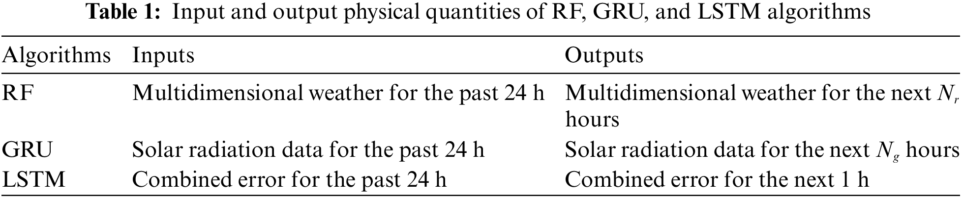
The processed composite error, weighted according to the inverse error proportion, serves as input for the LSTM network, enabling further optimization of the error. Leveraging its superior capacity for capturing long-term dependencies compared to GRU, LSTM adeptly learns the intrinsic patterns within the error sequence. Subsequently, the output from the LSTM network provides the prediction for solar radiation intensity in the upcoming hour. Following this prediction, the final estimate for solar radiation intensity is derived. Refer to Table 1 for a comprehensive overview of the input and output physical quantities associated with each algorithm in the proposed method.
The article employs four key indicators to assess the performance of the model:
(1) R² (coefficient of determination): R² serves as a metric for model fit, signifying the proportion of variation in the dependent variable explained by the model. Ranging from 0 to 1, a higher R² indicates a better fit to the data, while a lower R² implies a poorer fit.
where n is the number of samples;
(2) Root mean squared error (RMSE): the square root of the mean of the sum of the squares of differences between predicted and actual values serves as a measure of prediction accuracy. A smaller RMSE corresponds to better prediction performance.
where n is the number of samples;
(3) Mean absolute error (MAE): MAE represents the mean of the absolute differences between predicted and actual values. A smaller MAE reflects superior prediction performance.
where n is the number of samples;
(4) BIAS (Deviation): BIAS gauges the deviation between predicted and actual values, providing insights into the accuracy of prediction results. When BIAS is close to 0, it signifies accurate predictions. A BIAS greater than 0 indicates overestimation, while a BIAS less than 0 implies underestimation.
where n is the number of samples;
4 Experimental Results and Analysis
The simulation environment for this study is meticulously configured with an Intel Core i9-12900H processor, 32 GB of 6000 MHz RAM, a 64-bit Windows 11 operating system, and MATLAB R2021b as the software version. Within this well-defined environment, researchers conduct simulation experiments to assess the solar energy resource forecasting performance of the proposed method. To enhance the comparability of the simulation experiments, three groups of comparison algorithms are introduced: the RF model, GRU network, and LSTM network.
Jiangmen City (latitude 22°16′47″~22°17′03″N, longitude 113°03′30″~113°03′50″E) is located in the central-southern part of Guangdong Province, downstream of the Xijiang, in the Western Pearl River Delta. It falls under the subtropical marine climate category. Nestled downstream of the Xijiang River, in the western region of the Pearl River Delta, the city enjoys a subtropical maritime climate characterized by warmth and rainfall, devoid of snow throughout the year, and featuring minimal inter-annual temperature fluctuations. With 1838.6 annual sunshine hours and an average temperature of 22°C, Jiangmen serves as a representative location. Fig. 5 illustrates the city’s geographical coordinates.

Figure 5: Geographic location map of Jiangmen City
In terms of topography and geomorphology, Jiangmen City boasts a diverse landscape encompassing hills, plains, and river networks. The terrain gradually descends from north to south. The utilization of a dataset reflecting this intricate topographic and geomorphological makeup in simulation experiments is instrumental. The dataset allows for testing the adaptability of the proposed method across diverse terrains and evaluating their performance under varied application scenarios.
The experimental data include daily climate data from ground stations in China and daily field station solar irradiation intensity in the hills and mountains of Jiangmen City. This study specifically curated data spanning from May 13 2022, to November 11, 2022. The selected dataset comprises a comprehensive set of variables, including visibility (VIS), mean relative humidity (RHU-mean), minimum relative humidity (RHU-min), mean wind speed (WIN-mean), mean precipitation (PRE-mean), mean barometric pressure (PRS-mean), maximum pressure (PRS-max), minimum pressure (PRS-min), sunshine duration (SSD), mean temperature (TEM-mean), maximum temperature (TEM-max), minimum temperature (TEM-min), mean ground surface temperature (GST-mean), and solar radiation intensity (AD).
4.2 Performance of Random Forest Algorithm for Daily Solar Radiation Prediction
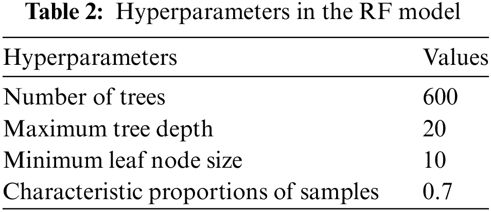
The optimal performance and generalization ability of the RF algorithm hinge on the careful selection of hyperparameters. Varied hyperparameter configurations can result in noteworthy disparities in model performance. To ensure the RF model attains its best potential, this study employs grid search to fine-tune its hyperparameters. The specifics of hyperparameter selection for the RF model are succinctly illustrated in Table 2.
In the random forest algorithm, feature importance assessment helps to identify the key features that have a large impact on the model prediction results, guide the feature selection and dimensionality reduction, and improve the model performance and generalization ability. At the same time, feature importance assessment also helps to enhance the interpretability of the model and better understand the relationship between features and the prediction process. Taking the solar irradiance intensity data for the hilly as an example, Fig. 6 shows the importance of each feature in meteorological data.
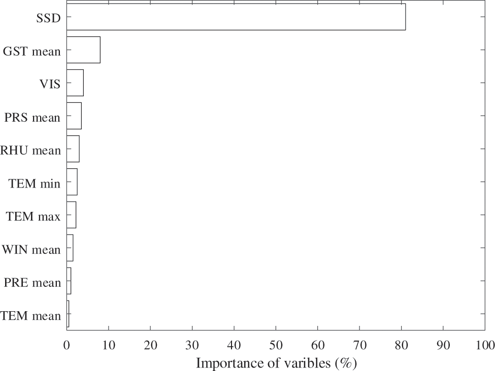
Figure 6: Feature importance map in random forest model prediction
As can be seen in Fig. 7, the SSD is considered to be the most critical variable, followed by GST-mean, VIS, PRS-mean, RHU-mean, TEM-min, TEM-max, WIN-mean, TEM-mean, PRE-mean, RHU-min, PRS-max, PRS-min, in descending order. The significance of SSD is 81%, which is consistent with the results of earlier studies. The importance of GST-mean was 8% and all other variables were less than 5%. Fig. 7 shows the performance of the RF model in predicting hourly solar radiation.

Figure 7: Scatter plot of solar radiation intensity predicted by random forest model
4.3 Performance of Gated Recurrent Unit for Daily Solar Radiation Prediction
This study employs grid search to tune the hyperparameters of the GRU network to obtain the best model performance. Table 3 demonstrates the selection of hyperparameters in the GRU model. Fig. 8 demonstrates the loss variation curve and RMSE variation curve during the training process of the GRU network. Fig. 9 demonstrates the scatter plot of solar radiation intensity predicted by the GRU model.
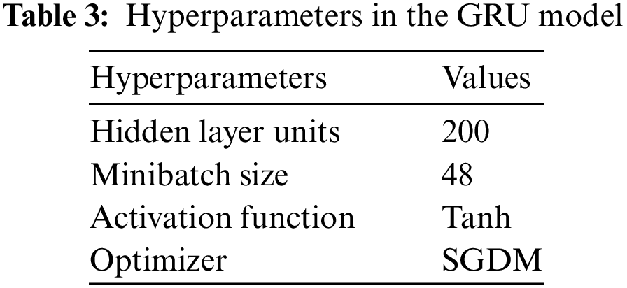
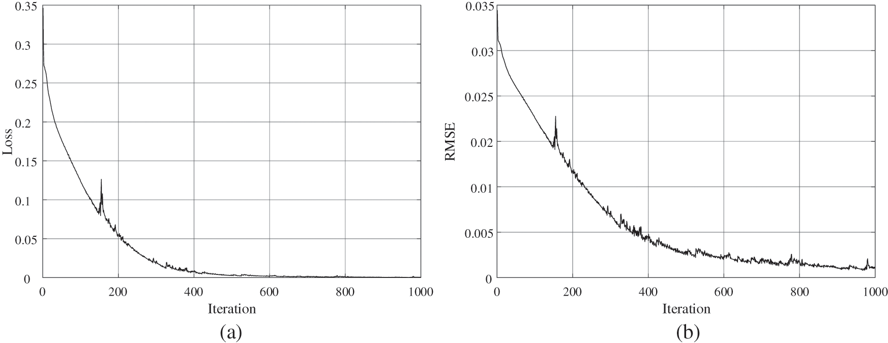
Figure 8: Training curves of GRU network: (a) RMSE variation curve during training; (b) LOSS variation curve during training

Figure 9: Scatter plot of solar radiation intensity predicted by GRU
4.4 Overall Prediction Performance of Proposed Method
The proposed method incorporates RF, GRU, and LSTM networks, and the combination of these models can fully utilize their respective strengths to achieve a highly accurate prediction of solar radiation intensity. Table 4 demonstrates the selection of hyperparameters for the algorithms included in the proposed method.
Fig. 10 visually presents the prediction outcomes generated by both the proposed algorithm and the comparison algorithm on hilly data. Notably, the proposed method leverages the synergies of Random Forest (RF), Gated Recurrent Unit (GRU), and Long Short-Term Memory (LSTM) networks, achieving a remarkable level of accuracy in forecasting solar radiation intensity. On the other hand, the comparison algorithms encompass RF, LSTM, GRU, support vector machines (SVM), orthogonal matching pursuit (OMP), extreme gradient boosting (XGB), and kernel ridge (KR).
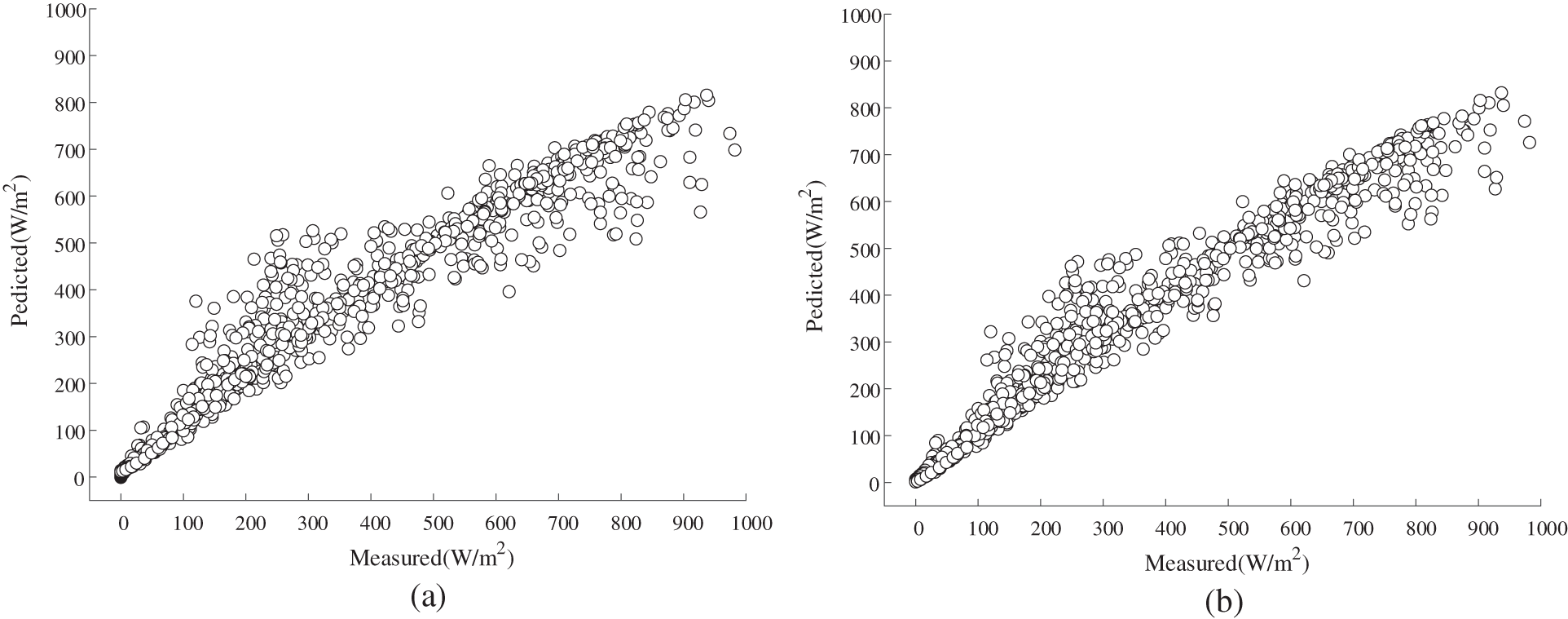

Figure 10: Scatterplots of solar radiation intensity results output by prediction algorithms: (a) scatterplot of prediction results of the proposed method; (b) scatterplot of prediction results of the RF; (c) scatterplot of prediction results of the GRU; (d) scatterplot of prediction results of the LSTM; (e) scatterplot of prediction results of the SVM; (f) scatterplot of prediction results of the OMP; (g) scatterplot of prediction results of the XGB; (h) scatterplot of prediction results of the KR
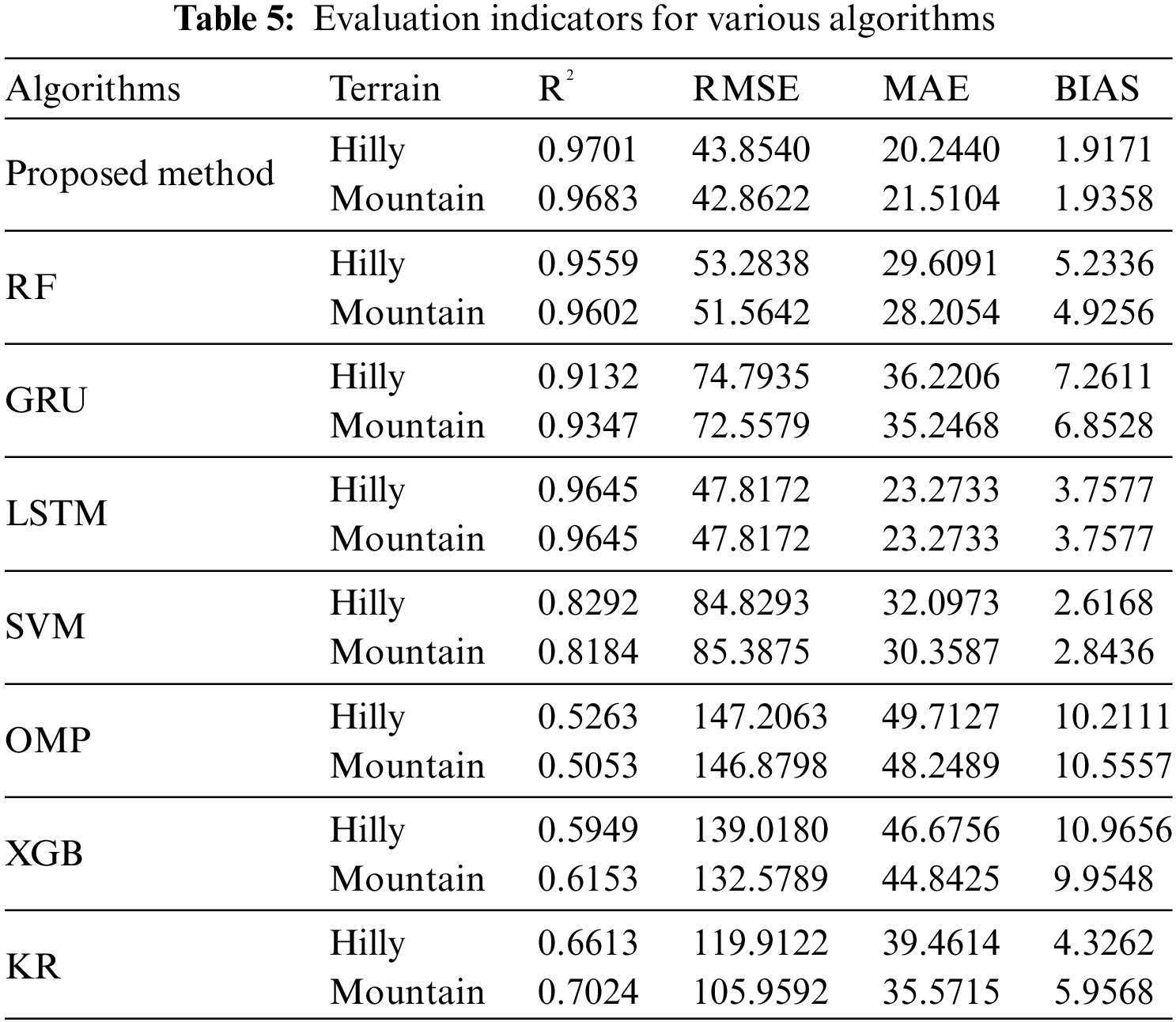
For a more comprehensive assessment, Table 5 encapsulates the evaluation metrics data for both the proposed algorithm and the comparative algorithms under different terrain landscapes. Analyzing the experimental results reveals that the proposed method exhibits superior fitting capabilities, particularly in predicting solar radiation data. Across all evaluation indices, the proposed method outshines the comparative algorithms, underscoring its heightened accuracy and reliability in photovoltaic resource assessment. These findings affirm the effectiveness of the proposed method, establishing it as a robust tool for guiding the siting and design of photovoltaic power plants.
The article focuses on the photovoltaic resource assessment method utilizing integrated deep learning. It begins by introducing the principles of three machine learning algorithms—RF, GRU, and LSTM. Subsequently, it innovatively combines integration and deep learning algorithms for photovoltaic resource assessment. The article concludes by comparing the advantages of the proposed method against individual machine learning algorithms through simulation results. The primary research contributions are as follows:
(1) Introduction of a photovoltaic resource assessment method based on integrated deep learning, a pioneering approach that combines integrated learning and deep learning methods. This method effectively enhances the accuracy and reliability of photovoltaic resource assessment by integrating RF, GRU, and LSTM.
(2) Exploration of a hierarchical forecasting framework’s performance, which merges multiple forecasting models to achieve more efficient and accurate predictions. Unlike traditional methods, this framework maximizes the strengths of each model, leveraging their respective advantages.
(3) Analysis of simulation results demonstrates that integrating RF and GRU prediction errors can mitigate biases from a single model caused by noise, outliers, or missing values. This enhances the model’s resistance to interference, ensuring more stable and effective prediction results.
Despite the high accuracy and adaptability demonstrated in experiments, the proposed photovoltaic resource assessment method has limitations. Future improvements and extensions could include: (I) Incorporating more types of meteorological data: The current dataset might lack comprehensive coverage of factors influencing photovoltaic resource assessment. Future research should consider including additional meteorological data, such as atmospheric pressure, humidity, and surface albedo, to enhance the model’s adaptability to complex meteorological conditions. (II) Temporal-spatial data fusion: Given the evident temporal-spatial characteristics of solar radiation, future research could explore combining spatial data with time-series data to better capture the temporal-spatial variations in solar radiation. (III) Exploring more deep learning models: Beyond GRU and LSTM, numerous other deep learning models, such as convolutional neural networks and graph neural networks, could find application in photovoltaic resource assessment. Future research should investigate the potential of these models in enhancing the accuracy and versatility of photovoltaic resource assessments.
Acknowledgement: None.
Funding Statement: The research is funded by Key-Area Research and Development Program Project of Guangdong Province (2021B0101230003) and China Southern Power Grid Science and Technology Project (ZBKJXM20220004).
Author Contributions: The authors confirm contribution to the paper as follows: study conception and design: Li L., Yang Z.; data collection: Yang X.; analysis and interpretation of results: Zhou Q., Yang P.; draft manuscript preparation: Zhou Q. All authors reviewed the results and approved the final version of the manuscript.
Availability of Data and Materials: The authors confirm that the data supporting the findings of this study are available within the article. And the additional data that support the findings of this study are available on request from the corresponding author, upon reasonable request.
Conflicts of Interest: The authors declare that they have no conflicts of interest to report regarding the present study.
References
1. Nathwani, J., Kammen, D. M. (2019). Affordable energy for humanity: A global movement to support universal clean energy access. Proceedings of the IEEE, 107(9), 1780–1789. [Google Scholar]
2. Breyer, C., Bogdanov, D., Gulagi, A., Aghahosseini, A., Barbosa, L. S. N. S. et al. (2017). On the role of solar photovoltaics in global energy transition scenarios. Progress in Photovoltaics: Research and Applications, 25(8), 727–745. [Google Scholar]
3. Choi, Y., Suh, J., Kim, S. M. (2019). GIS-based solar radiation mapping, site evaluation, and potential assessment: A review. Applied Sciences, 9(9), 1960. [Google Scholar]
4. Stökler, S., Schillings, C., Kraas, B. (2009). Solar resource assessment study for Pakistan. Renewable and Sustainable Energy Reviews, 58, 1184–1188. [Google Scholar]
5. Tolabi, H. B., Moradi, M. H., Ayob, S. B. M. (2014). A review on classification and comparison of different models in solar radiation estimation. International Journal of Energy Research, 38(6), 689–701. [Google Scholar]
6. Yang, D., Wang, W., Xia, X. (2022). A concise overview on solar resource assessment and forecasting. Advances in Atmospheric Sciences, 39(8), 1239–1251. [Google Scholar]
7. Tang, W., Qin, J., Yang, K., Liu, W., Lu, N. et al. (2016). Retrieving high-resolution surface solar radiation with cloud parameters derived by combining MODIS and MTSAT data. Atmospheric Chemistry and Physics, 16(4), 2543–2557. [Google Scholar]
8. Yeom, J. M., Deo, R. C., Adamwoski, J. F., Chae, T., Kim, D. S. et al. (2020). Exploring solar and wind energy resources in North Korea with COMS MI geostationary satellite data coupled with numerical weather prediction reanalysis variables. Renewable and Sustainable Energy Reviews, 119, 109570. [Google Scholar]
9. Huld, T., Müller, R., Gambardella, A. (2012). A new solar radiation database for estimating PV performance in Europe and Africa. Solar Energy, 86(6), 1803–1815. [Google Scholar]
10. Baser, F., Demirhan, H. (2017). A fuzzy regression with support vector machine approach to the estimation of horizontal global solar radiation. Energy, 123, 229–240. [Google Scholar]
11. Ibrahim, I. A., Khatib, T. (2017). A novel hybrid model for hourly global solar radiation prediction using random forests technique and firefly algorithm. Energy Conversion and Management, 138, 413–425. [Google Scholar]
12. Wang, F., Zhang, Z., Chai, H., Yu, Y., Lu, X. et al. (2019). Deep learning based irradiance mapping model for solar PV power forecasting using sky image. 2019 IEEE Industry Applications Society Annual Meeting, pp. 1–9. Maryland, USA, IEEE. [Google Scholar]
13. Ge, Y., Nan, Y., Bai, L. (2019). A hybrid prediction model for solar radiation based on long short-term memory, empirical mode decomposition, and solar profiles for energy harvesting wireless sensor networks. Energies, 12(24), 4762. [Google Scholar]
14. Acikgoz, H. (2022). A novel approach based on integration of convolutional neural networks and deep feature selection for short-term solar radiation forecasting. Applied Energy, 305, 117912. [Google Scholar]
15. Mellit, A. (2008). Artificial Intelligence technique for modelling and forecasting of solar radiation data: A review. International Journal of Artificial Intelligence and Soft Computing, 1(1), 52–76. [Google Scholar]
16. Sansine, V., Ortega, P., Hissel, D., Hopuare, M. (2022). Solar irradiance probabilistic forecasting using machine learning, metaheuristic models and numerical weather predictions. Sustainability, 14(22), 15260. [Google Scholar]
17. Gaboitaolelwe, J., Zungeru, A. M., Yahya, A. (2023). Machine learning based solar photovoltaic power forecasting: A review and comparison. IEEE Access, 11, 40820–40845. [Google Scholar]
18. Devaraj, J., Madurai Elavarasan, R., Shafiullah, G. M., Jamal, T., Khan, I. (2021). A holistic review on energy forecasting using big data and deep learning models. International Journal of Energy Research, 45(9), 13489–13530. [Google Scholar]
19. Kumari, P., Toshniwal, D. (2021). Deep learning models for solar irradiance forecasting: A comprehensive review. Journal of Cleaner Production, 318, 128566. [Google Scholar]
20. Biau, G., Scornet, E. (2016). A random forest guided tour. Test, 25, 197–227. [Google Scholar]
21. Chen, J., Li, K., Tang, Z., Bilal, K., Yu, S. et al. (2016). A parallel random forest algorithm for big data in a spark cloud computing environment. IEEE Transactions on Parallel and Distributed Systems, 28(4), 919–933. [Google Scholar]
22. Genuer, R., Poggi, J. M., Tuleau-Malot, C., Vialaneix, N. V. (2017). Random forests for big data. Big Data Research, 9, 28–46. [Google Scholar]
23. Graves, A., Graves, A. (2012). Long short-term memory. Supervised Sequence Labelling with Recurrent Neural Networks, 385, 37–45. [Google Scholar]
24. Pascanu, R., Mikolov, T., Bengio, Y. (2013). On the difficulty of training recurrent neural networks. International Conference on Machine Learning, pp. 1310–1318. Atlanta, USA. [Google Scholar]
25. Greff, K., Srivastava, R. K., Koutník, J., Steunebrink, B. R., Schmidhuber, J. (2016). LSTM: A search space odyssey. IEEE Transactions on Neural Networks and Learning Systems, 28(10), 2222–2232. [Google Scholar] [PubMed]
26. Chung, J., Gulcehre, C., Cho, K. H., Bengio, Y. (2014). Empirical evaluation of gated recurrent neural networks on sequence modeling. arXiv preprint arXiv:1412.3555. [Google Scholar]
27. Chen, T., Guestrin, C. (2016). XGBoost: A scalable tree boosting system. Proceedings of the 22nd ACM Sigkdd International Conference on Knowledge Discovery and Data Mining, pp. 785–794. New York, NY, USA. [Google Scholar]
28. Strobl, C., Boulesteix, A. L., Zeileis, A., Hothorn, T., Bioinformatics BMC. (2007). Bias in random forest variable importance measures: Illustrations, sources and a solution. BMC Bioinformatics, 8(1), 1–21. [Google Scholar]
Cite This Article
 Copyright © 2024 The Author(s). Published by Tech Science Press.
This work is licensed under a Creative Commons Attribution 4.0 International License , which permits unrestricted use, distribution, and reproduction in any medium, provided the original work is properly cited.
 Downloads
 Citation Tools