The Emergency Control Method for Multi-Scenario Sub-Synchronous Oscillation in Wind Power Grid Integration Systems Based on Transfer Learning

1  Introduction

With the rapid development of new energy technologies, the share of renewable energy in modern power systems is continuously rising, and power electronic equipment is being more widely applied in power grids [1–3]. Renewable energy sources, such as wind and solar power, are increasingly integrated into the grid on a large scale through electronic devices, fundamentally altering the grid’s structure and dynamic characteristics, and introducing new stability challenges, particularly sub-synchronous oscillations linked to wind power integration [4,5]. Currently, wind power grid integration systems mainly suppress sub-synchronous oscillations by optimizing turbine control strategies at the unit level and by incorporating devices like static synchronous compensators [6,7]. However, due to the complex topology and coupling dynamics of wind power integration systems, these suppression methods can sometimes fail, leading to difficulties in reliably controlling sub-synchronous oscillations [8]. Therefore, proactive emergency controls and load-shedding measures are needed on the grid side to prevent the spread of sub-synchronous oscillations and to avoid potential equipment damage or system failures.

Extensive research has been conducted domestically and internationally on emergency control for sub-synchronous oscillation in wind power grid integration systems. Reference [9] proposed a generalized harmonic compensation control strategy for an active power filter with a supercapacitor, which effectively suppresses sub-synchronous oscillations by injecting generalized harmonic currents, including reactive and oscillation currents. Reference [10] reframed the machine-shedding problem as finding the optimal shedding rate by calculating the increment in the real part of the system’s aggregate impedance. Reference [11] addresses the issue of sub-synchronous resonance in a series-compensated DFIG-based wind power plant and proposes its mitigation through the use of a Battery Energy Storage-based Damping Controller. Reference [12] introduces a novel approach to mitigating sub-synchronous oscillations in series-compensated transmission lines by employing a resonant controller in combination with a control loop for the doubly fed induction generator. Reference [13] aimed to enhance system damping by establishing shedding criteria based on frequency-domain impedance criteria and measured complex impedance modulus and phase angle information, recommending methods for offline screening of effective machine groups for emergency control and determining the shedding sequence. However, these methods are based on ideal system conditions and may not adequately address the variable operation modes and complex environments of real-world systems. This paper innovatively integrates transfer learning (TL) with deep reinforcement learning (DRL) to address two critical challenges in wind power grid emergency control: (1) the high dependency of traditional DRL on massive target scenario data, and (2) the limited adaptability of fixed-scenario models to dynamic real-world environments. The proposed framework leverages a pre-trained DRL model from source scenarios (e.g., historical simulations with known wind speeds and grid topologies) and employs Maximum Mean Discrepancy (MMD) to quantify distribution shifts between source and target domains. By aligning feature representations via MMD, the proposed framework enables dynamic knowledge transfer across diverse scenarios, thereby reducing data dependency, enhancing generalization capabilities, and improving adaptability to real-world operational conditions.

In recent years, artificial intelligence technology has matured rapidly, with wide-spread applications in areas such as robotics control, autonomous driving, and electronic sports games [14–17]. Transfer Learning (TF), an emerging field in artificial intelligence, focuses on the core concept of transferring previously acquired knowledge to similar or related domains. Traditional machine learning methods require building separate models for different problems, which is both inefficient and leads to unnecessary computational resource expenditure in practical engineering applications. Transfer learning, however, uses experience or pre-trained models from prior tasks to accelerate convergence towards effective strategies, reducing the need for relearning and enhancing adaptability to new tasks or environments. This approach minimizes training time and computational demands, making the training process more efficient and stable, and has demonstrated impressive performance in fields like text processing, image classification, and intelligent planning. Transfer learning is currently applied in power system optimization control and stability analysis. For example, Reference [18] presented a deep neural network architecture with shared hidden layers for wind speed prediction, improving short-term prediction accuracy through transfer learning techniques. Reference [19] proposed a graph convolutional network-based deep reinforcement learning framework to address topology changes in power system voltage stability control design. These studies illustrate the effectiveness of transfer learning in transferring knowledge from previous domains to new applications.

Addressing the aforementioned issues, this study constructs a sub-synchronous oscillation emergency control model for wind power grid integration systems under fixed scenarios, using deep reinforcement learning. A reward evaluation system is developed based on the system’s active power oscillation pattern, incorporating penalty functions for the number of machine-shedding rounds and the number of machines shed to mitigate economic losses and grid security risks associated with excessive one-time turbine shedding. Additionally, transfer learning is integrated into the model training to enhance its generalization capability for managing the complex scenarios typical of real-world wind power grid integration systems. By employing the Maximum Mean Discrepancy (MMD) algorithm to calculate the distribution differences between source and target data, the model’s online decision-making reliability is further improved. Finally, the effectiveness of the proposed transfer-learning-based emergency control method for multi-scenario sub-synchronous oscillations in wind power grid integration systems is analyzed using the New England 39-bus system.

2  Deep Reinforcement Learning Model

2.1 The DRL Decision Model for Sub-Synchronous Oscillation

The initial definitions of the agent’s state, action, and reward function are crucial in modeling the emergency control problem of sub-synchronous oscillation in wind power grid integration systems as a deep reinforcement learning (DRL) problem, as they significantly impact the performance and effectiveness of the DRL model. Therefore, the state space, action space, and reward function are designed as follows:

2.1.1 State Space

In deep reinforcement learning, the agent perceives the system’s current operating conditions through the input state space data. This study defines the state space by selecting the voltage magnitude and phase at the system’s network nodes, as well as the current magnitude and phase at the network branches. For a system with N nodes and L branches, the agent’s state space can be expressed as:

S=[VNj,θNj,ILi,θLi](1)

In the above equation, VNj represents the voltage magnitude of the j-th node, ILi represents the current magnitude of the i-th branch, θNj represents the voltage phase of the j-th node, θLi represents the current phase of the i-th branch.

2.1.2 Action Space

The action space of the agent includes all possible machine-shedding actions for the system. Therefore, the action space A is defined as follows:

A=[a1,a2,…,am](2)

In the equation, a1,…am represents the machine-shedding control actions.

To enhance the agent’s training effectiveness, the machine-shedding control action space is uniformly discretized. For the wind power system, the discretized action indices are denoted as follows:

Ac={0,c=0aeu,1≤c≤bh(3)

where b denotes the wind farm index, u represents the proportion of wind farm shedding, u=1,2,…h, c is the action number represented as a natural number, and aeu denotes the discretized machine-shedding control actions (e=1,2,…b). There are bh groups of actions in total.

2.1.3 Reward Function

This study proposes dividing the reward function into two main categories: short-term rewards and long-term rewards. Short-term rewards evaluate whether the current system state satisfies specific constraint conditions, while long-term rewards assess the system’s stability following the implementation of the control strategy. The specific design principles for the reward function include:

Rt={Rc,st∈SstableRp,st∉Sstable0,st∈SconstrainRf,st∉Sconstrain(4)

where st represents the state obtained by the agent, including synchronous phasor voltage and current data; Sstable denotes the set of states where sub-synchronous oscillations have been mitigated after the implementation of machine-shedding actions; Sconstrain represents system constraints; Rc is the long-term reward value for mitigating sub-synchronous oscillations after implementing the machine-shedding control strategy; Rf denotes the short-term reward function after each round of machine-shedding control actions; and Rp represents the penalty value for system instability due to oscillations after implementing the machine-shedding control strategy.

(1) Long-Term Stability Criterion

The long-term stability criterion guides the agent’s decision-making by assessing the system’s overall stability, enabling the agent to learn and optimize control strategies for sustained stable operation. When sub-synchronous oscillations occur in a wind power grid integration system, oscillations in the active power on the tie line can be consistently observed. By monitoring variations in the tie line’s active power, the stability level of the system after applying control actions can be assessed. First, record the adjacent maximum (Pmaxk) and minimum (Pmink) values of the active power on the tie line (k∈1,2,3,⋯). Then, calculate the oscillation amplitude (Ak) at different times as shown in Eq. (5).

Ak=Pmaxk−Pmink(5)

This set of discrete points is denoted as AK. Fit AK using an exponential function, as shown in Eq. (6).

A(t)=q1⋅exp⁡(q2t)+q3(6)

where q1, q2, and q3 are the parameters of the exponential function obtained from fitting AK. Differentiating Eq. (6) yields Eq. (7):

A′(t)=q1q2⋅exp⁡(q2t)(7)

Analyzing the above equation, we can see that: When the coefficients satisfy condition q1q2<0, the oscillation slope is negative, the amplitude gradually converges, and the system exhibits long-term stability. The larger the value of |q1q2|, the stronger the system damping, and the higher the system stability. When the coefficients satisfy condition q1q2>0, the oscillation slope is positive, the amplitude gradually diverges, and the system becomes unstable. When the coefficients satisfy condition q1q2=0, the oscillation slope is approximately zero, resulting in constant amplitude oscillations.

When the coefficients satisfy the condition q1q2<0, the oscillation slope is negative, leading to a gradual convergence in amplitude, which indicates long-term stability in the system. A larger absolute value of |q1q2| corresponds to stronger system damping and greater stability. Conversely, when the coefficients satisfy q1q2>0, the oscillation slope is positive, causing the amplitude to gradually diverge, resulting in system instability. If the coefficients satisfy q1q2=0, the oscillation slope is approximately zero, leading to constant amplitude oscillations.

(2) Short-Term Reward Function

The short-term reward function in this study consists of two components: a reward for limiting the number of machines shed and a reward for constraining the number of machine-shedding rounds. The expressions are as follows:

Rf=rcost+rstep(8)

The reward function for constraining the number of machines shed involves a weighted summation of the amount shed, representing the cost associated with the machine-shedding action. This constraint function guides the agent in developing more effective machine-shedding strategies, achieving an optimal balance between system stability and economic efficiency. The specific expression is as follows:

rc=∑k=1bcgak(9)

where ak represents the amount of shedding on the grid side, and cg represents the penalty coefficient for machine shedding.

The reward for constraining the number of machine-shedding rounds is designed to encourage the agent to minimize the total number of control rounds. This constraint function aids in achieving faster mitigation of system oscillations and prevents larger-scale losses. The specific expression is as follows:

rstep=cnNstep,Nstep=1,2,…Nmax(10)

where Nmax is the preset maximum number of control rounds, cn is the penalty coefficient for the number of machine-shedding rounds, and Nstep is the actual number of machine-shedding control rounds.

2.2 DRL Agent Neural Network

As shown in Fig. 1, the estimated neural network uses operational observation data from the power system as inputs, with the outputs representing the values of various actions. To accelerate the model’s convergence and improve training stability, data of different magnitudes are normalized to the same range. This study employs the Deep Q-Network (DQN) algorithm to construct the deep reinforcement learning network. The DQN algorithm selects the optimal action by estimating the value of each action generated by the network. For the DQN algorithm, this paper constructs a five-layer fully connected neural network as the estimation network. The estimation network consists of three hidden layers to adequately capture the complex dynamics between the power system’s state and action values. The number of neurons in the input layer corresponds to the dimensionality of the state space, while the number of neurons in the output layer corresponds to the dimensionality of the action space. The number of neurons in the hidden layers is set to 256. The structure of the deep Q target network is the same as the estimation network, with the target network’s weight parameters inherited from the estimation network’s weight parameters at regular intervals. The discount factor for the DQN algorithm is set to 0.90, the learning rate for the neural network is set to 0.0005, and the ε-greedy policy increases with the number of training steps, reaching a maximum value of 0.99.

at=argmaxq∗(s,a;θ)(11)

where q∗(s,a) represents the optimal action value function, at denotes the control action considered optimal by the agent, and θ refers to the parameters of the estimated network.

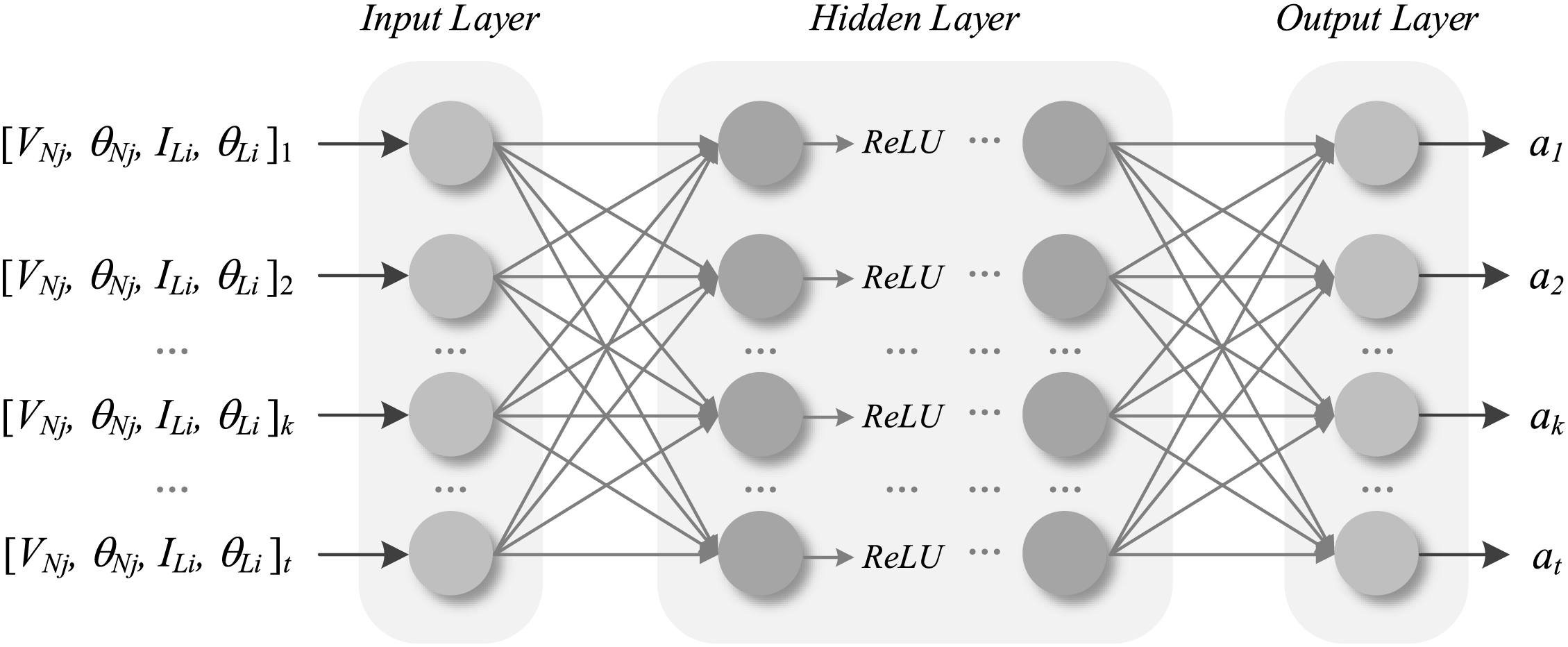
Figure 1: Estimating the network structure

The loss function of the estimated network in the DQN algorithm is defined as:

Lt(θt)=Es,a∼p(.)[(yt−Q(s,a;θt))2](12)

where s,a∼P(.) represents the probability distribution over state and action yt denotes the label function, which is the target function for the i-th iteration; Q(s,a;θt) represents the output of the estimated network at the i-th iteration.

The target function yt represents the training objective of the estimated network, which changes with the network weights, and is defined as follows:

yt=E[rt+γmaxa′Q(s′,a′;θt−1)|s,a](13)

where rt represents the reward obtained in the t-th iteration; maxa′Q(s′,a′;θt−1) denotes the maximum estimated network output corresponding to the action sequence a′.

By differentiating the loss function Lt(θt) with respect to the estimated network parameters θt, the gradient of the loss function concerning the parameters of the estimated neural network in the t-th iteration can be obtained, as shown in the following equation:

∇θtLt(θt)=Es,a∼p(.)[(r+γmaxa′Q(s′,a′;θt−1)−Q(s,a;θt))∇θtQ(s,a;θt)](14)

where ∇θtQ(s,a;θt) represents the gradient of the estimated neural network output with respect to the neural network parameters during the t-th iteration.

By using the gradient descent method to minimize the loss function Lt(θt), the internal parameters θt of the estimated neural network are updated, thus completing the iterative update of the estimated neural network.

The update process of the DQN algorithm neural network is illustrated in Fig. 2. The specific steps are as follows:

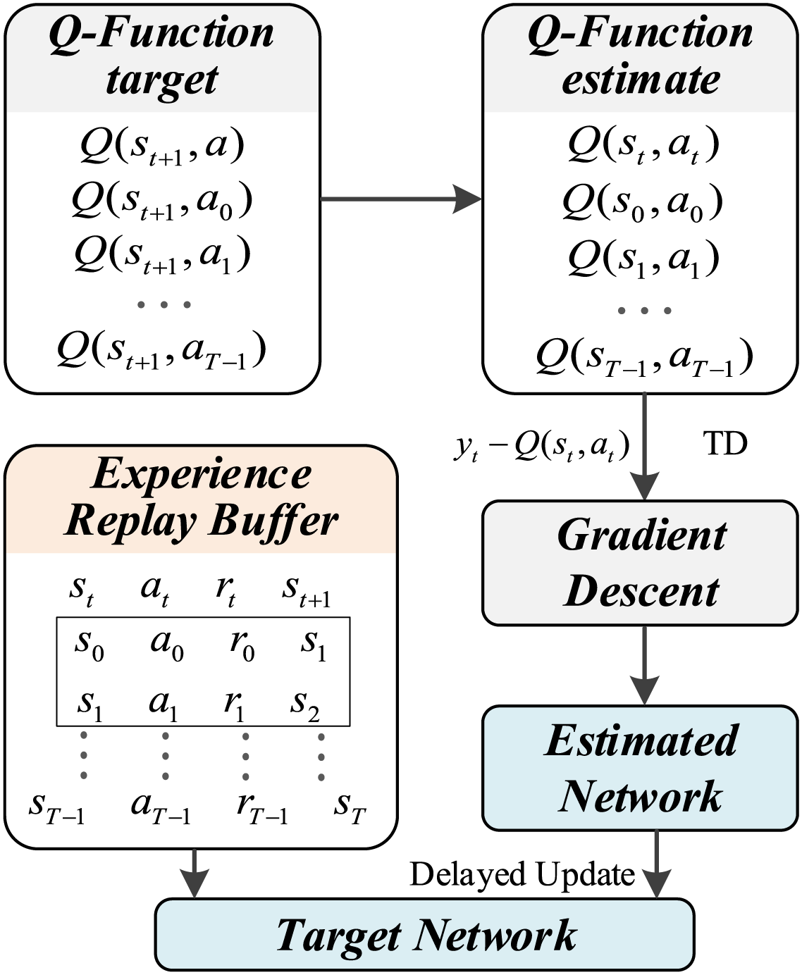
Figure 2: DQN algorithm neural network update method

Step 1: The agent executes actions in the environment based on a greedy policy, collecting experience tuples <st,at,rt,st+1>.

Step 2: The collected experiences are stored in an experience replay buffer. A batch of experiences is randomly sampled from the buffer for learning.

Step 3: For each sampled experience, the target network is used to calculate the maximum Q-value for the next state. The target Q-value is then calculated based on the reward and discount factor γ.

Step 4: The estimated network calculates the Q-values for each action in the current state. The loss function Lt(θt) is then computed, and the gradient descent method is used to minimize the loss function, updating the weights of the estimated network.

Step 5: Every few episodes, the weights of the estimated network are copied to the target network.

The DQN algorithm has commendable online decision-making capabilities but also exhibits certain limitations. Consequently, various improved algorithms have been proposed, such as the Rainbow algorithm, which combines the Double DQN method, Dueling DQN method, and Dropout mechanism. This combination has demonstrated superior convergence performance. Therefore, this study aims to enhance existing algorithms to achieve an overall improvement in model training performance.

2.2.1 State Space

In the traditional DQN algorithm, the action-value function (Q-value) is updated by maximizing the Q-value from the evaluation network. However, this approach can lead to overestimation, potentially resulting in inflated values for certain actions, which adversely affects the selection of optimal actions. The Double DQN method addresses this by separating action selection from value estimation, effectively reducing the impact of overestimation. In the Double DQN algorithm, the calculation of the training target value is performed using both the estimation network and the target network. Specifically, rather than using the target network to select the action with the maximum Q-value, the estimation network is used to identify the action that maximizes the Q-value for the next state. The Q-value of this action is then calculated with the target network and used to update the estimation network. Consequently, the Q-value update during training is modified as follows:

QDouble=[rt+1+γQ(st+1,arg⁡maxQ(st+1,a;w);w−)−Q(st,at;w)](15)

2.2.2 Dueling DQN Algorithm

Dueling DQN represents an enhancement to the DQN neural network. In some states, an action may have minimal influence on state transitions, while in others, certain actions can significantly impact the state itself. Therefore, it is important to consider the intrinsic value of the state. The Dueling DQN method addresses this by modifying the output layer of the estimation network into two branches—one representing the state value and the other representing the action advantage. This adjustment aims to improve the algorithm’s convergence performance. The modified neural network architecture of the Dueling DQN algorithm is shown in Fig. 3.

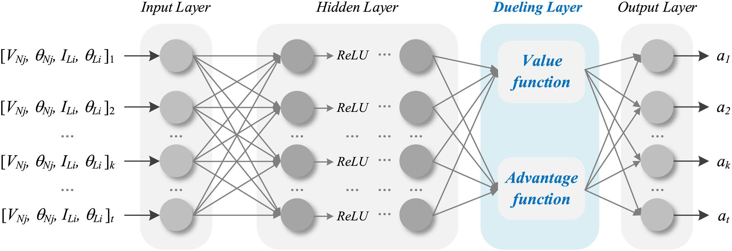
Figure 3: Dueling network architecture

The optimal action-value function and the optimal state-value function are defined, along with the advantage function as follows:

A∗(s,a)=Q∗(s,a)−V∗(s)(16)

In the DQN algorithm, the optimal state-value function is approximated using a neural network, while the advantage function is also approximated using a neural network. Consequently, the Q-value is calculated as follows:

Q(s,a;w)=V(s;wV)+A(s,a;wA)−maxaA(s,a;wA)(17)

Due to fluctuations in the state value function and the advantage function, the Q-value may remain unchanged even if these two functions vary, leading to ambiguity in uniquely determining the state value and advantage functions through training the Q-network. This could result in multiple combinations without achieving improved convergence. To address this, the maximum value of the advantage function is subtracted to obtain better results. In practice, using the mean value has been shown to yield superior outcomes, and the Q-value calculation is modified as follows:

QDueling(st,at)=v(st)+[A(st,at)−1|A|∑atA(st,at)](18)

2.2.3 Dropout Mechanism

In machine learning models, an excessive number of parameters combined with limited training samples can lead to overfitting. This issue is particularly prevalent during the training of emergency control strategies in a single scenario, where excessive training iterations often cause the agent to almost exclusively select actions with the highest reward value, reducing the exploration of alternative strategies. As a result, the agent learns a fixed strategy, converging to a local optimum, which hinders adaptation to complex multi-scenario problems. To mitigate overfitting during neural network training, the Dropout mechanism is commonly employed. In the Dropout mechanism, certain neurons are deactivated with a specified probability during forward propagation, meaning they do not participate in parameter calculations. This approach prevents specific features from being effective only under certain conditions, reducing the joint effect of correlated hidden nodes and thereby enhancing the model’s generalization capability.

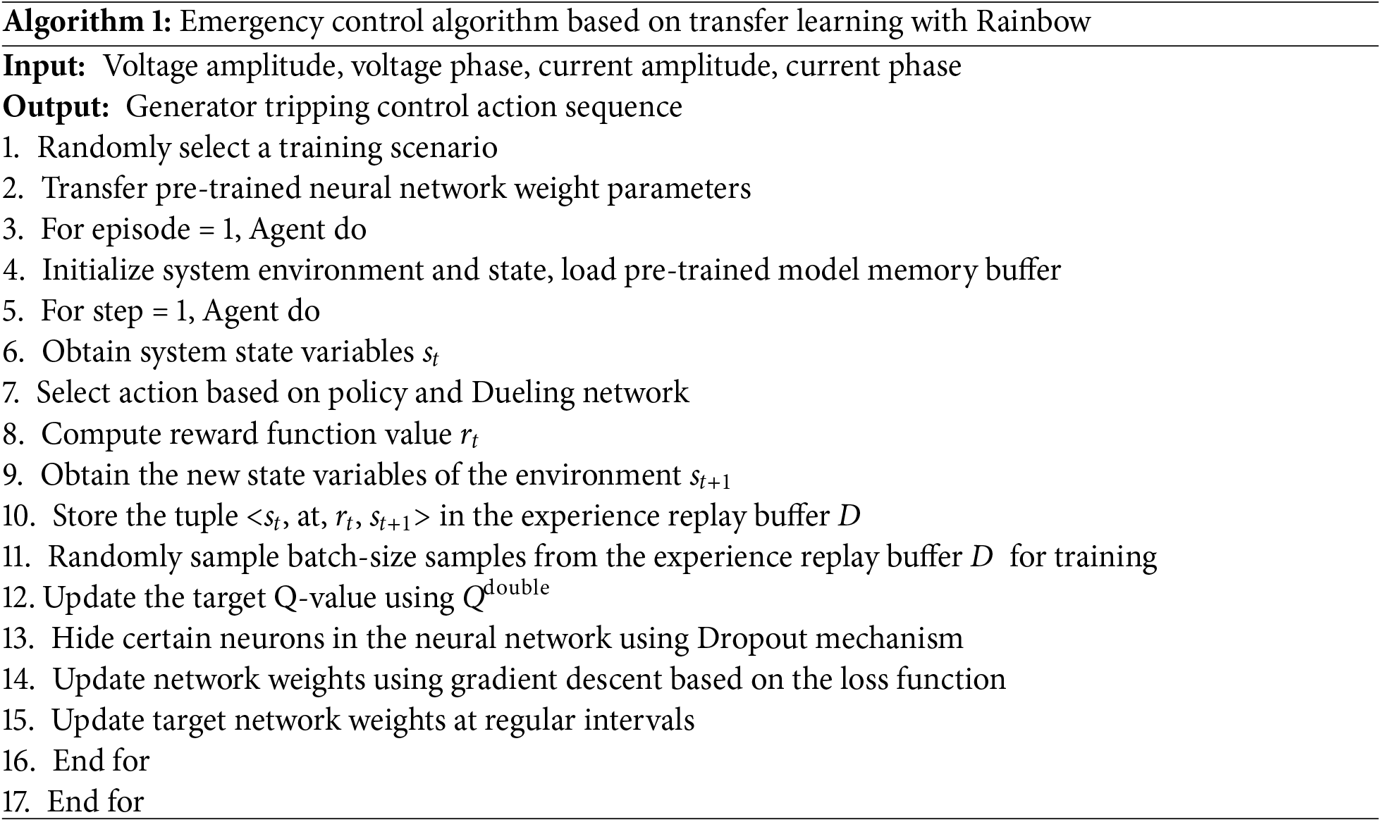
2.2.4 Emergency Control Strategy Algorithm Based on Rainbow

After pre-training, the pre-trained estimation network model, target network model, and experience buffer are stored. In the full training phase, the model parameters are transferred to a new model, and after fine-tuning the output layer parameters, the model is used for comprehensive training. The workflow of the Rainbow algorithm for multi-scenario emergency control is outlined in Algorithm 1.

3  Transfer Learning Model

The goal of transfer learning is to improve or accelerate the learning and performance of a deep reinforcement learning model in the target task and domain by leveraging knowledge and experience from the source task and domain. A basic example is illustrated in Fig. 4.

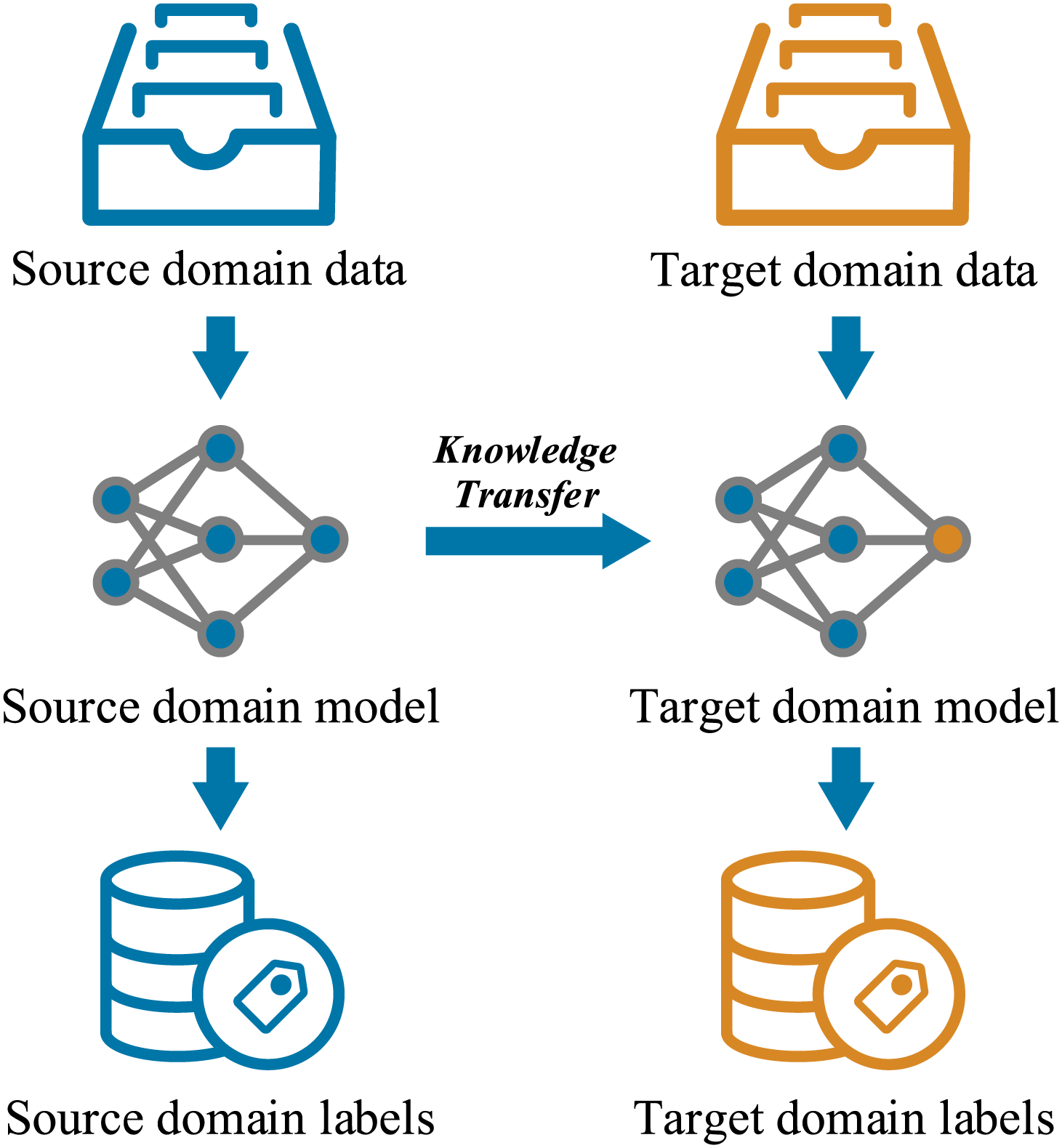
Figure 4: Example of transfer learning model

In this approach, the target domain model corresponds to the multi-scenario emergency control model to be developed, while the source domain model consists of historical data or a simulation model of a single operating condition.

MMD is a statistical method used to measure the difference between two data distributions. The core principle is that if two distributions are identical, their means in a high-dimensional feature space should align perfectly. MMD quantifies the similarity between distributions by computing the norm of the mean difference. In wind power grid integration systems, the distributions of source scenario training data and target scenario operational data may differ due to factors such as wind speed and grid topology. Directly applying the model trained on the source scenario may lead to decision failures. By utilizing MMD filtering, the model is permitted to make decisions only within a reliable distribution range, preventing control failures caused by discrepancies between scenarios.

3.1 Maximum Mean Discrepancy Algorithm

Suppose F is a set of continuous functions on the sample space, and p and q are two independent probability distributions. Then MMD can be expressed as:

MMD[F,p,q]=supf∈F(Ep[f(x)]−Eq[f(y)])(19)

The empirical estimate of MMD is given by:

MMD[F,X,Y]=supf∈F(1m∑i=1mf(xi)−1n∑i=1nf(yi))(20)

where X and Y are two datasets sampled from distributions p and q, respectively; m and n are the sizes of the datasets.

Analyzing the above equation shows that if the function set F can be arbitrarily defined, two identical distributions might yield a large MMD value under a specific function set. Therefore, certain constraints must be applied.

Define the function set F as any vector within the unit ball in the Reproducing Kernel Hilbert Space (RKHS) [20]. As a complete inner product space, f(x) can be represented as the inner product of vector f in the RKHS with vector ϕ(x) in the same space, specifically expressed as:

f(x)=⟨f,ϕ(x)⟩H(21)

Based on the above definition and utilizing the properties of the Reproducing Kernel Hilbert Space (RKHS), μp can be used to replace Ep[ϕ(x)] as follows:

MMD[F,p,q]=sup‖f‖H≤1(Ep[f(x)]−Eq[f(y)])=sup‖f‖H≤1(Ep[⟨ϕ(x),f⟩H]−Eq[⟨ϕ(y),f⟩H])=sup‖f‖H≤1(μp−μq,f)H=‖up−uq‖H(22)

Squaring the MMD gives:

MMD2[F,p,q]=⟨μp,μp⟩H+⟨μq,μq⟩H−2⟨μp,μq⟩H=Ep⟨ϕ(x),ϕ(x′)⟩H+Eq⟨ϕ(y),ϕ(y′)⟩H−2Ep,q⟨ϕ(x),ϕ(y)⟩H(23)

Expressing the inner product using the kernel function k(x,x′):

k(x,x′)=e−‖x−x′‖22σ2(24)

Thus, the solving formula for MMD can be obtained as shown in Eq. (25).

MMD[F,X,Y]=[1m(m−1)∑i≠jmk(xi,xj)+1n(n−1)∑i≠jnk(yi,yj)−2mn∑i,j=1m,nk(xi,yj)]12(25)

From the above derivation, it can be seen that MMD obtains the distance between the points corresponding to the two distributions in the RKHS.

3.2 Transfer Learning Model for Multi-Scenario Oscillation Emergency Control in Wind Power Grid Integration Systems

3.2.1 Pre-Training in Fixed Scenarios

Pre-training in fixed scenarios aims to train the model on a fixed oscillation scenario so that it can understand the basic operations and control strategies of the power grid. The specific steps are as follows:

Step 1: Initialize the agent’s policy network parameters.

Step 2: Train the agent using an offline interactive training platform with Python and Simulink.

Step 3: Save the experience replay buffer, estimated network, target network models, and parameters of the pre-trained model.

3.2.2 Transfer Learning Training for Multi-Scenario

In implementing multi-scenario emergency control strategies for wind power grid integration systems, the transfer learning training phase for multi-scenario plays a crucial role. The core purpose of this phase is to adapt the fixed-scenario pre-trained model to different operating modes and conditions, thus improving the system’s adaptability to new scenarios and the accuracy of control strategies. Compared to fixed-scenario pre-training, this phase focuses more on the model’s generalization ability to scenario changes. The emergency control framework based on transfer learning is illustrated in Fig. 5, and the specific steps are as follows:

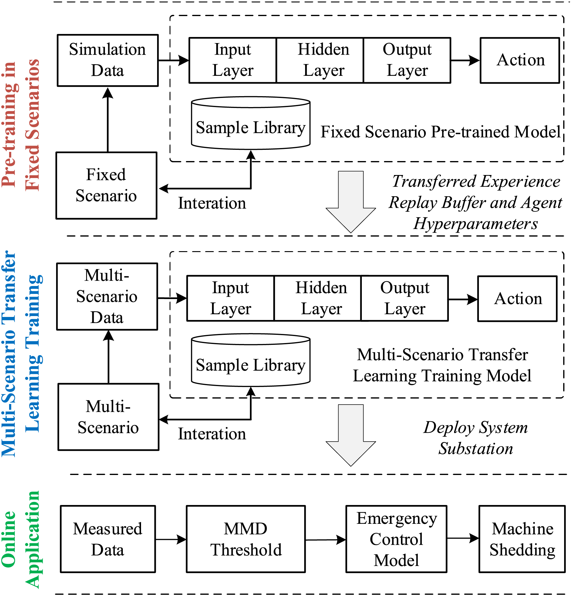
Figure 5: Transfer learning framework for emergency control of sub-synchronous oscillations in wind power grid integration systems

Step 1: During the full training phase, transfer the neural network model and parameters from the pre-training phase to a new agent. To enhance the model’s generalization ability, transfer the fully connected layer parameters of the pre-trained model to the new model and use the Dropout mechanism to disable some connections between neurons, reducing the risk of overfitting.

Step 2: When initializing the training scenario, select a scenario with the risk of sub-synchronous oscillation as the target scenario for transfer learning training until the model’s reward function value converges.

3.2.3 Online Emergency Control Based on MMD

If the system experiences sub-synchronous oscillation, use the system node voltage magnitudes, phases, and branch current magnitudes, phases datasets as target domain data. Calculate the MMD value between the target domain data and the source domain data used for transfer learning training. If the MMD value is less than the threshold a, invoke the agent model, and the agent will provide the optimal machine-shedding strategy based on the policy network.

4  Case Study

In this study, the wind power grid integration system is modeled using Simulink simulation software, while the deep reinforcement learning model is built with TensorFlow 2.9, Google’s deep learning framework. The DQN algorithm is implemented in Python, taking advantage of Python’s ability to interface with Simulink, allowing the DRL agent to learn through interaction with the environment. The experiments in this study were conducted on a system running Windows 10 22H2 64-bit. It features an Intel Core i5-13600K processor with 12 cores at 5.1 GHz, 16 GB of RAM, and an NVIDIA GeForce RTX 4060 Ti GPU with 16 GB of VRAM for accelerated computations. Data storage was provided by a 1 TB solid-state drive (SSD), supporting efficient model training and simulations.

4.1 Pre-Training in Fixed Scenarios

In this case study, the New England 39-bus system was modified to include wind farms WF1 to WF9 connected at nodes 4, 5, 7, 8, 16, 17, 18, 26, and 27. Additionally, series compensation capacitors were added to lines L4–5 and L17–27. The improved system retains the original 39 nodes and 46 branches but exhibits significant changes in network topology due to the integration of wind farms and series compensation capacitors. The network topology is shown in Fig. 6.

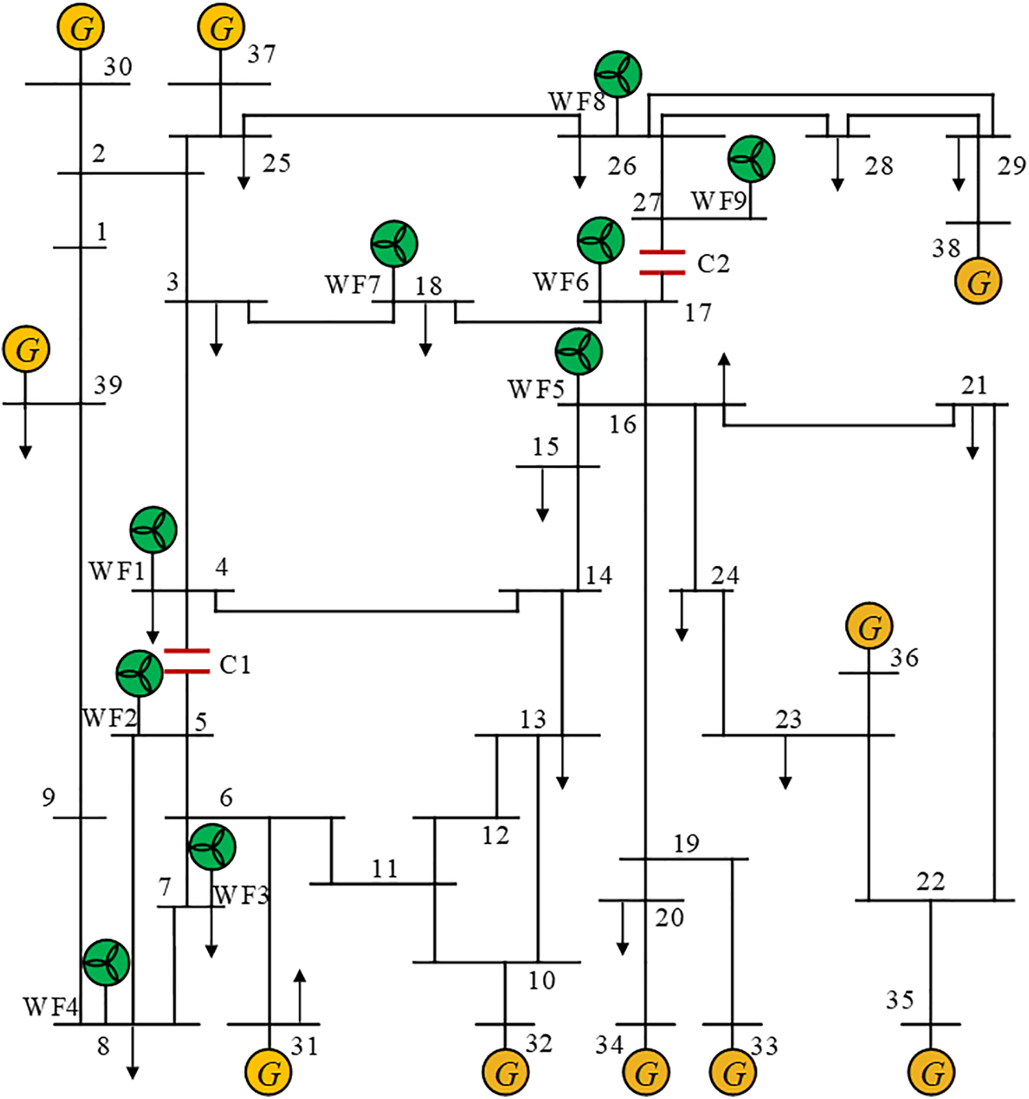
Figure 6: Modified New England 39-bus system

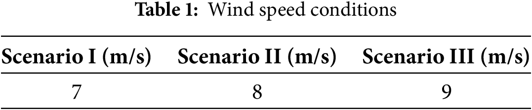
In the modified New England 39-bus system, 99 scenarios with sub-synchronous oscillations were generated. Based on these scenarios, adjustments were made to wind speed conditions, resulting in a total of 20,000 sub-synchronous oscillation scenarios. The wind speed conditions, series compensation capacity, and wind turbine output are detailed in Tables 1–3, respectively.

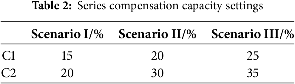
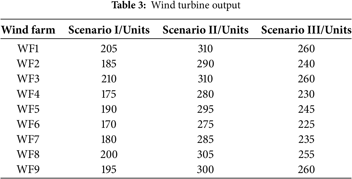
The scenarios with oscillations are shown in Table 4.

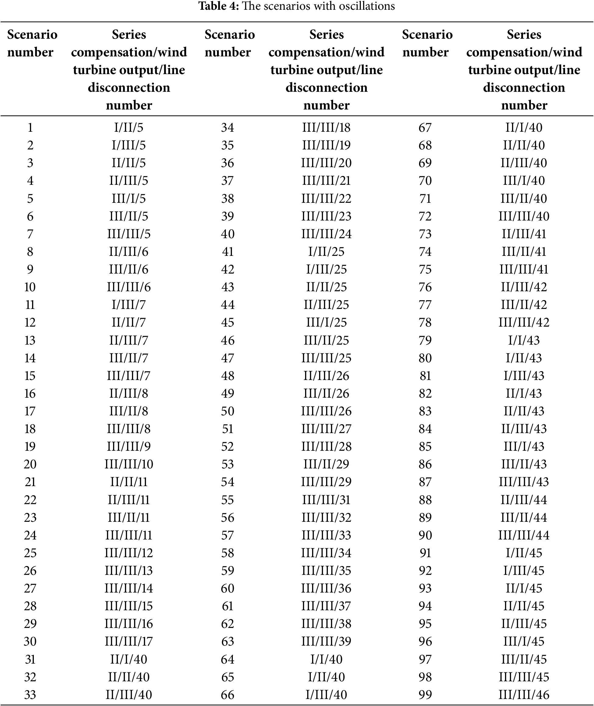
The fixed scenario pre-training uses condition 64. The changes in the reward function during the agent’s training process are shown in Fig. 7.

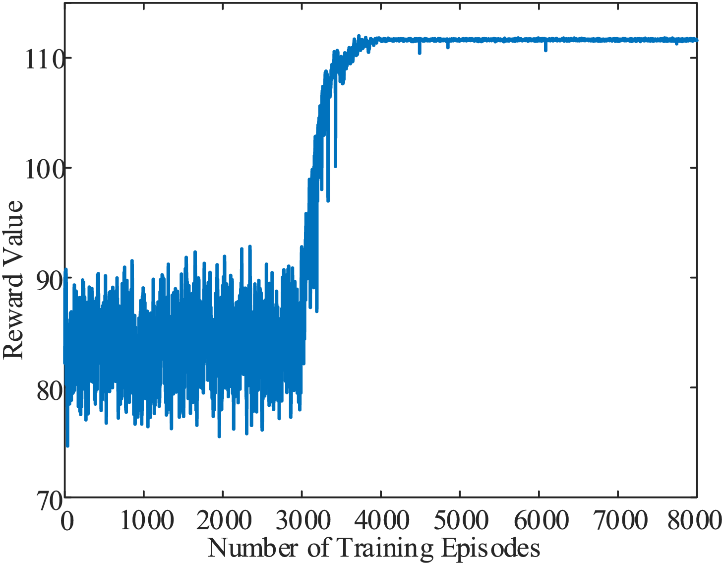
Figure 7: Changes in reward function during agent training

As shown in the Fig. 7, after 3000 episodes, the agent’s exploration rate decreases, and it increasingly relies on decisions from the policy network. The reward function begins to converge and fully stabilizes after 4000 episodes, at which point the agent learns a stable control strategy. The emergency control strategy developed by the agent in response to sub-synchronous oscillations caused by the disconnection of line 40 in this case study is presented in Table 5.

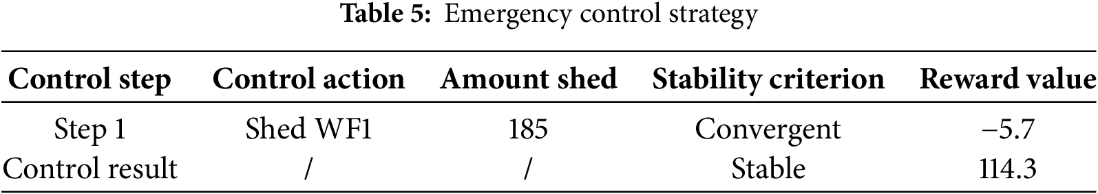
At 6 s, wind farm WF1 sheds 185 turbines, restoring system stability. The voltage at node 16 and the current in branch L16–17, before and after the implementation of emergency control measures, are shown in Fig. 8. It can be observed that after applying the emergency control strategy provided by the DRL model, sub-synchronous oscillations are quickly and reliably eliminated.

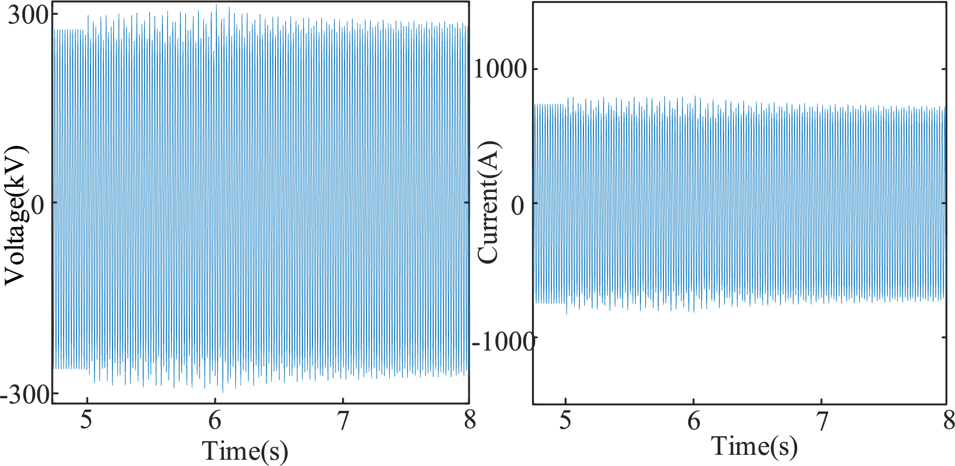
Figure 8: Voltage and current curves of the system

4.2 Transfer Learning Training Phase

The target network policy structure, estimated network policy structure, experience replay buffer, and neural network hyperparameters from the pre-trained fixed scenario model are transferred. A total of 15,000 oscillation scenarios are randomly selected as the training environment for transfer learning. Fig. 9 displays the reward value curve during the initial training session of the transfer learning model.

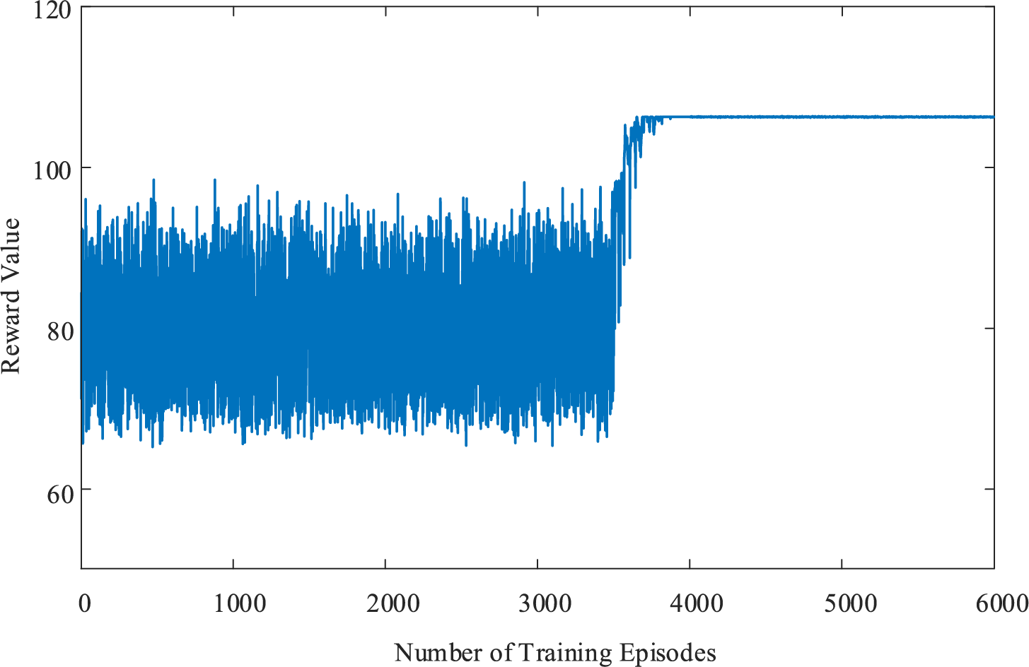
Figure 9: Reward function curve in the early stage of transfer learning

As shown in the Fig. 9, during the initial stage of transfer learning, the agent cannot immediately learn the optimal control strategy due to changes in the training scenarios. By adjusting the exploration coefficient, the agent’s exploration rate is increased, enabling it to better learn optimal strategies across different scenarios. After 3500 episodes, the agent’s exploration rate decreases, and it increasingly relies on decisions from the policy network, with the reward function beginning to converge.

As the training progresses, the agent’s exploration coefficient is gradually reduced, decreasing the necessary exploration process required in the initial stages. Fig. 10 shows the reward value curve of the fully trained transfer learning model. It can be seen that the agent is able to provide actions with high reward values based on its own strategy from the early stages. At this point, the model has formed a relatively stable neural network structure and parameters. When applied online, setting the exploration coefficient of the model to zero will enable the emergency control model to output the correct machine-shedding decisions.

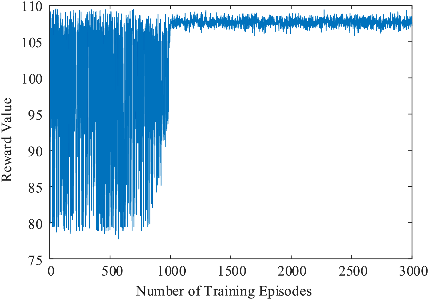
Figure 10: Reward function curve of the fully trained transfer learning model

To more intuitively demonstrate the advantages of transfer learning, an emergency control model without transfer learning is used as a control group, with the results shown in Fig. 11. In the early training stages, the control group’s average reward function value is significantly lower than that of the model with transfer learning. After the exploration rate decreases, the control group without transfer learning is unable to develop a stable neural network structure and parameters, resulting in large fluctuations in the reward function and an inability to accomplish the task of online emergency control for sub-synchronous oscillations in the wind power grid integration system.

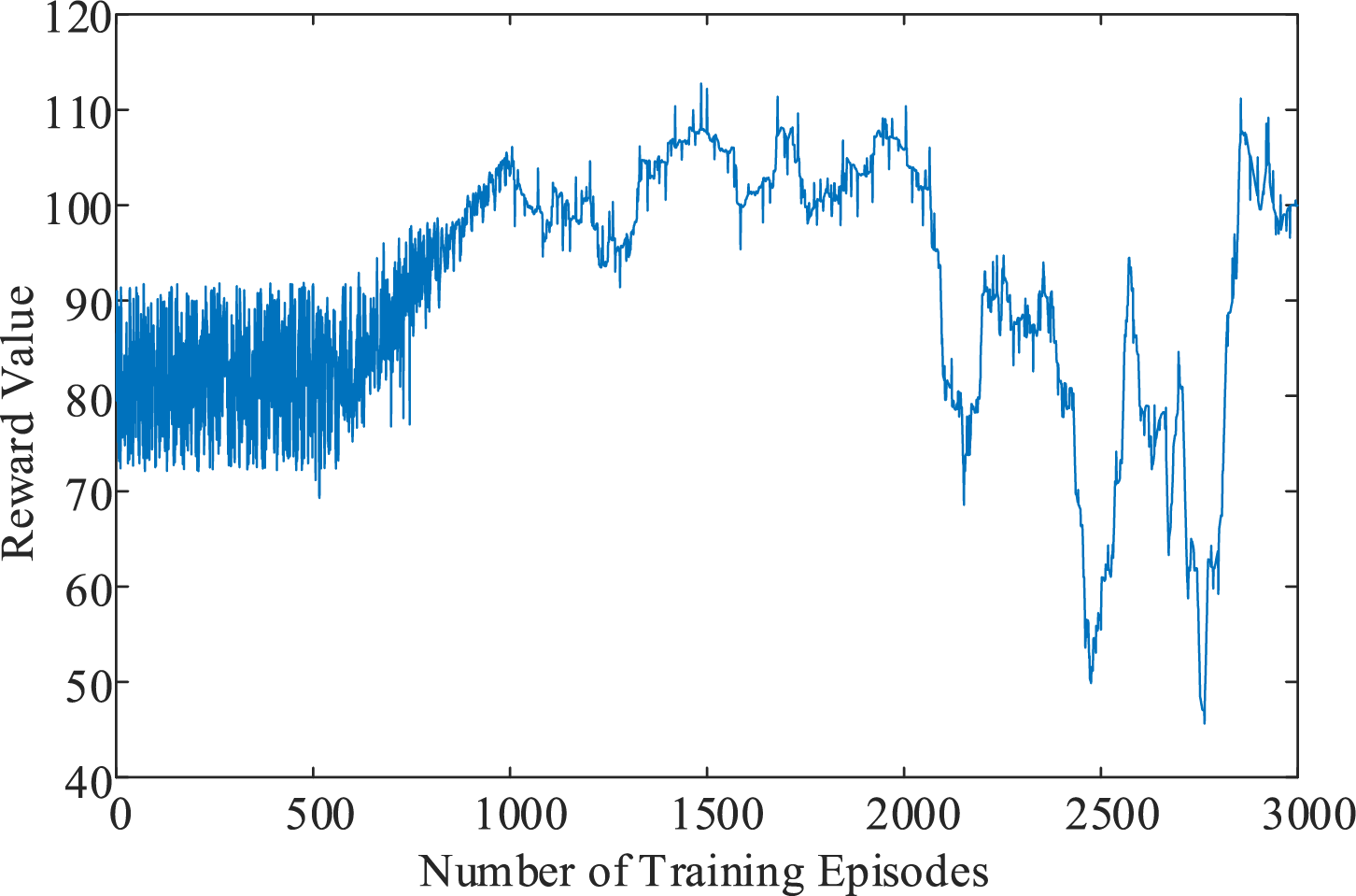
Figure 11: Comparison of reward function curves between transfer learning model and control group

Applying the sub-synchronous oscillation emergency control model, trained with complete transfer learning, to an actual wind power grid integration system may encounter issues if there are significant differences between the current system’s topology or operating mode and the training scenarios, which can prevent the model from providing accurate decisions. Therefore, after detecting oscillations, it is essential to calculate the Maximum Mean Discrepancy (MMD) value between the current system state variables and the transfer learning data. Based on the MMD value, it can be determined whether to use the decisions provided by the emergency control model. This study compares the decision reward values of the transfer learning model across oscillation scenarios with varying MMD values, as shown in Table 6.

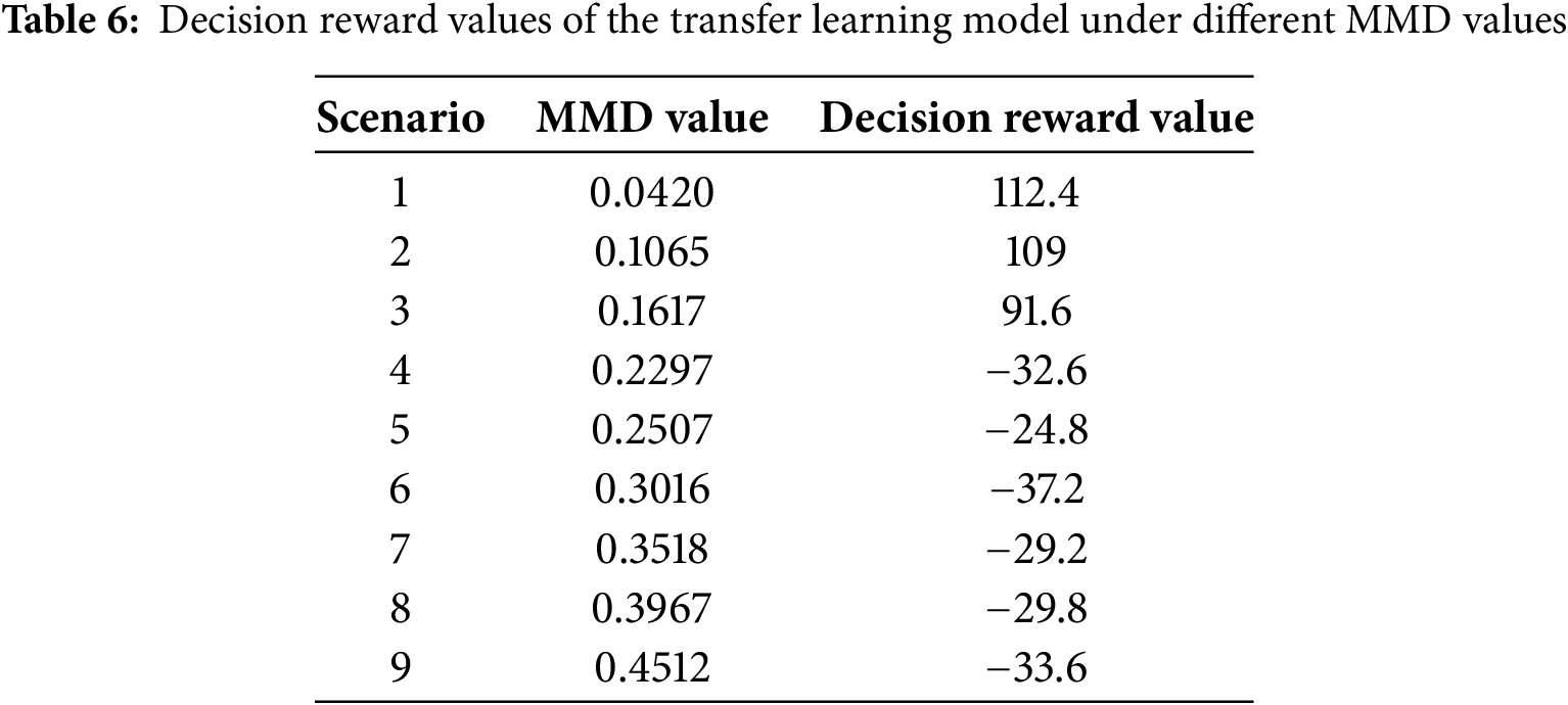
The reward values here are the actual rewards for single actions, not the moving average values.

As shown in Table 6, in entirely new scenarios, the model can provide correct machine-shedding decisions if the threshold a is relatively small. However, when the threshold a is large, the input data from the new scenario deviates significantly from the data distribution used during transfer learning training, preventing the model from reliably making correct machine-shedding decisions. Consequently, this study selects a threshold a of 0.15.

To validate the effectiveness of the proposed method, a new oscillation condition 96, which was not used in training, is set. The wind speed conditions are shown in Table 7.

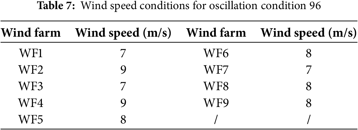
The MMD value for this scenario is calculated to be 0.054, which is less than 0.15. Thus, the emergency control model is activated to mitigate the oscillation. After inputting the synchronous phasor data of node voltage and current into the emergency control model, the decisions provided by the model are shown in Table 8.

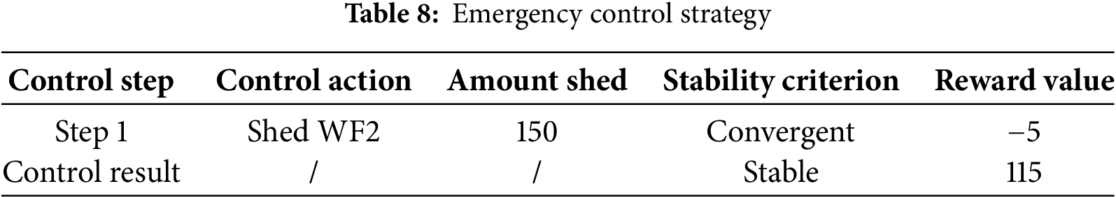
At 11 s, wind farm WF2 sheds 150 turbines, restoring system stability. The voltage at nodes, branch currents, and system power variation curves before and after implementing emergency control measures are shown in Figs. 12 and 13. These figures demonstrate that the multi-scenario sub-synchronous oscillation emergency control model for wind power grid integration systems, based on transfer learning, can promptly provide machine-shedding strategies and effectively eliminate system oscillations in new scenarios.

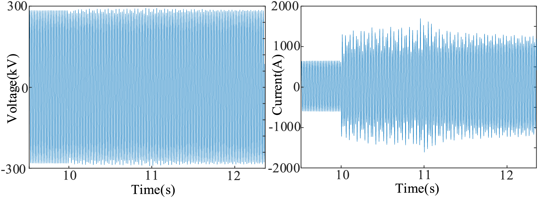
Figure 12: Voltage and current curves of the system before and after emergency control

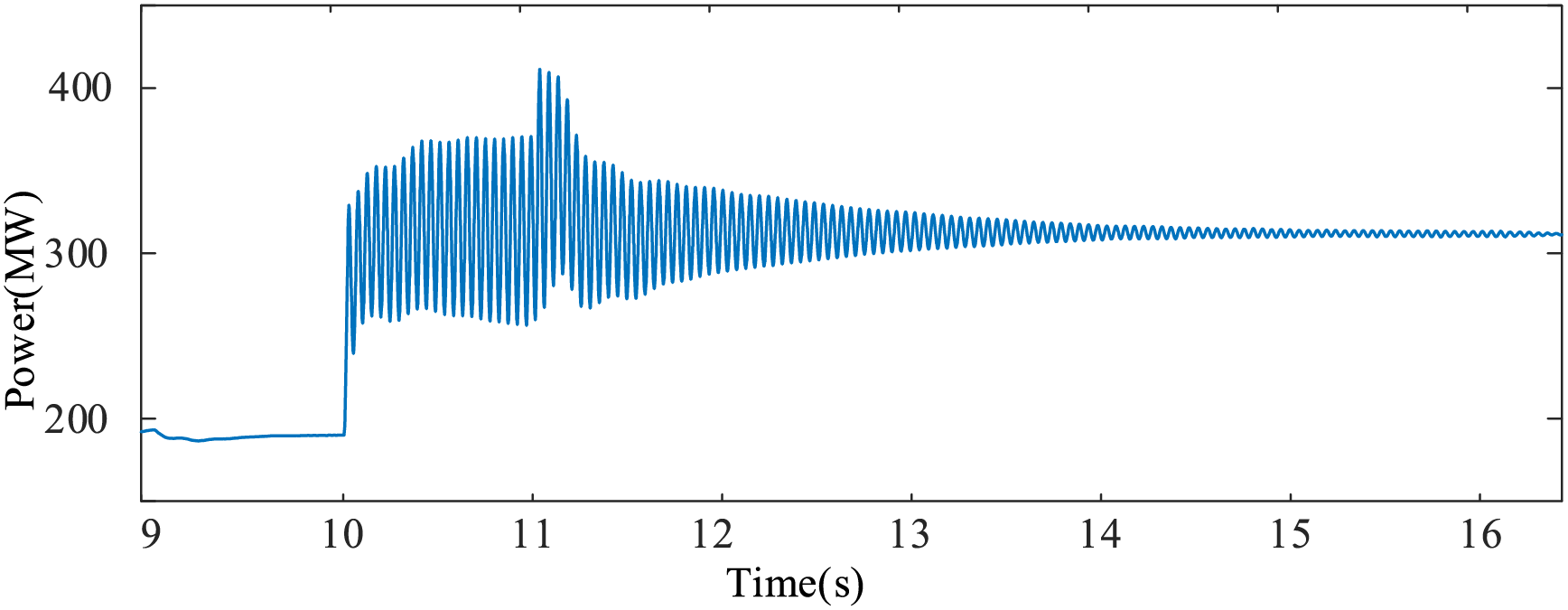
Figure 13: System power variation curves before and after emergency control

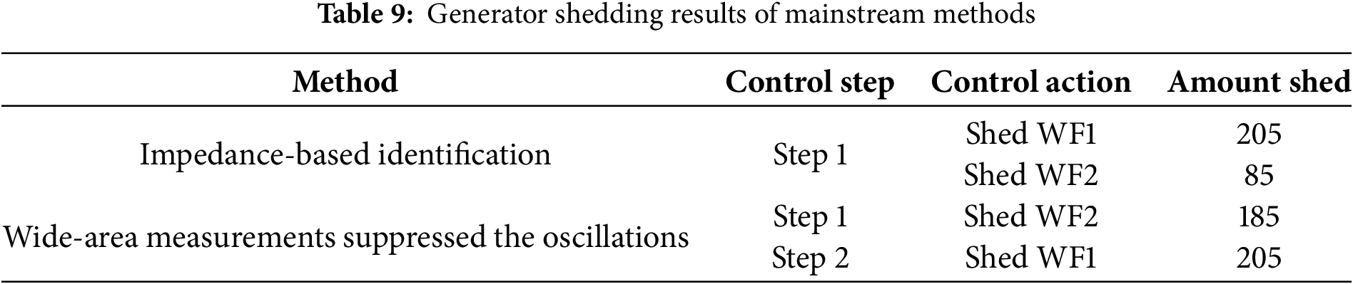
Table 9 presents the results of the current mainstream methods for sub-synchronous oscillation-based emergency generator shedding in wind power grid integration systems. It can be observed that the impedance-based identification method successfully suppressed the oscillations after one round of generator shedding. However, this method resulted in the shedding of 205 turbines from WF1 and 85 turbines from WF2. The dynamic generator shedding method based on wide-area measurements suppressed the oscillations after two rounds of generator shedding, involving the shedding of 185 turbines from WF2 and 205 turbines from WF1, totaling 390 turbines. In summary, it is evident that the proposed method in this paper achieves rapid suppression of oscillations while maximizing the retention of turbine numbers.

5  Conclusions

This study presents an emergency control method for sub-synchronous oscillations in wind power grid integration systems, based on transfer learning. First, a fixed-scenario emergency control model for sub-synchronous oscillations is constructed using deep reinforcement learning. A reward evaluation system is developed based on the oscillation pattern of the system’s active power, with penalty functions for the number of machine-shedding rounds and the number of machines shed, aiming to minimize economic losses and grid security risks associated with excessive one-time turbine shedding. Additionally, transfer learning is integrated into the model training to improve its generalization capability for handling the complex scenarios typical of actual wind power grid integration systems. The Maximum Mean Discrepancy (MMD) algorithm is introduced to calculate distribution differences between the source and target data, enhancing the model’s reliability in online decision-making. Finally, the proposed method is validated using the New England 39-bus system simulation. Results demonstrate that this method can provide fast and effective machine-shedding commands in scenarios that meet the threshold.

The sub-synchronous emergency control method proposed in this paper may encounter extreme situations in practical applications where the system state does not meet the MMD threshold requirements. Currently, this can only be addressed through manual determination for emergency generator shedding control under such conditions. Future research could combine data-driven and physics-based models to investigate emergency control strategies for sub-synchronous oscillations in the full scenario of wind power grid integration.

Acknowledgement: Not applicable.

Funding Statement: This research was funded by Sponsorship of Science and Technology Project of State Grid Xinjiang Electric Power Co., Ltd., grant number SGXJ0000TKJS2400168.

Author Contributions: Conceptualization: Qing Zhu, Denghui Guo and Rui Ruan; methodology: Qing Zhu, Denghui Guo, Rui Ruan and Zhidong Chai; software: Denghui Guo and Rui Ruan; validation: Chaoqun Wang and Zhiwen Guan; formal analysis: Qing Zhu; investigation: Qing Zhu; resources: Denghui Guo; data curation: Rui Ruan; writing—original draft preparation: Chaoqun Wang; writing—review and editing: Chaoqun Wang; visualization: Zhiwen Guan; supervision: Qing Zhu; project administration: Qing Zhu; funding acquisition: Qing Zhu, Denghui Guo, Rui Ruan and Zhidong Chai. All authors reviewed the results and approved the final version of the manuscript.

Availability of Data and Materials: Data will be made available on request.

Ethics Approval: Not applicable.

Conflicts of Interest: The authors declare no conflicts of interest to report regarding the present study.

References

1. Sun D, Qian Z, Shen W, Zhou K, Jin N, Chen Q. Mechanism analysis of multiple disturbance factors and study of suppression strategies of DFIG grid-side converters caused by sub-synchronous oscillation. Electronics. 2023;12(10):2293. doi:10.3390/electronics12102293. [Google Scholar] [CrossRef]

2. Ma J, Lyu L, Man J, Chen M, Cheng Y. Noise-like-signal-based sub-synchronous oscillation prediction for a wind farm with doubly-fed induction generators. Electronics. 2024;13(11):2200. doi:10.3390/electronics13112200. [Google Scholar] [CrossRef]

3. Liu H, Xie X, Gao X, Liu H, Li Y. Stability analysis of SSR in multiple wind farms connected to series-compensated systems using impedance network model. IEEE Trans Power Syst. 2018;33(3):3118–28. doi:10.1109/TPWRS.2017.2764159. [Google Scholar] [CrossRef]

4. Liu H, Xie X, He J, Xu T, Yu Z, Wang C, et al. Subsynchronous interaction between direct-drive PMSG based wind farms and weak AC networks. IEEE Trans Power Syst. 2017;32(6):4708–20. doi:10.1109/tpwrs.2017.2682197. [Google Scholar] [CrossRef]

5. Zhan Y, Xie X, Wang X, Zi P, Wang L. Injection-space security region for sub/super-synchronous oscillation in wind power integrated power systems. IEEE Trans Power Syst. 2024;39(2):3912–20. doi:10.1109/TPWRS.2023.3287289. [Google Scholar] [CrossRef]

6. Du W, Dong W, Wang H, Cao J. Dynamic aggregation of same wind turbine generators in parallel connection for studying oscillation stability of a wind farm. IEEE Trans Power Syst. 2019;34(6):4694–705. doi:10.1109/TPWRS.2019.2920413. [Google Scholar] [CrossRef]

7. He G, Wang W, Wang H. Coordination control method for preventing sub/super synchronous oscillations of multi-wind farm systems. CSEE J Power Energy Syst. 2023;9(5):1655–65. doi:10.17775/CSEEJPES.2020.06550. [Google Scholar] [CrossRef]

8. Shair J, Xie X, Yang J, Li J, Li H. Adaptive damping control of subsynchronous oscillation in DFIG-based wind farms connected to series-compensated network. IEEE Trans Power Deliv. 2022;37(2):1036–49. doi:10.1109/tpwrd.2021.3076053. [Google Scholar] [CrossRef]

9. Pang B, Si Q, Jiang P, Liao K, Zhu X, Yang J, et al. Review of the analysis and suppression for high-frequency oscillations of the grid-connected wind power generation system. Trans Electr Mach Syst. 2024;8(2):127–42. doi:10.30941/cestems.2024.00025. [Google Scholar] [CrossRef]

10. Li G, Ma F, Wu C, Li M, Guerrero JM, Wong MC. A generalized harmonic compensation control strategy for mitigating subsynchronous oscillation in synchronverter based wind farm connected to series compensated transmission line. IEEE Trans Power Syst. 2023;38(3):2610–20. doi:10.1109/TPWRS.2022.3191061. [Google Scholar] [CrossRef]

11. Xie X, Zhan Y, Shair J, Ka Z, Chang X. Identifying the source of subsynchronous control interaction via wide-area monitoring of sub/super-synchronous power flows. IEEE Trans Power Deliv. 2020;35(5):2177–85. doi:10.1109/TPWRD.2019.2963336. [Google Scholar] [CrossRef]

12. Verma N, Kumar N, Kumar R. Battery energy storage-based system damping controller for alleviating sub-synchronous oscillations in a DFIG-based wind power plant. Prot Control Mod Power Syst. 2023;8(1):32. doi:10.1186/s41601-023-00309-7. [Google Scholar] [CrossRef]

13. Touti E, Abdeen M, El-Dabah MA, Kraiem H, Agwa AM, Alanazi A, et al. Sub-synchronous oscillation mitigation for series-compensated DFIG-based wind farm using resonant controller. IEEE Access. 2024;12:66185–95. doi:10.1109/access.2024.3394507. [Google Scholar] [CrossRef]

14. Najmaei N, Kermani MR. Applications of artificial intelligence in safe human-robot interactions. IEEE Trans Syst Man Cybern B Cybern. 2011;41(2):448–59. doi:10.1109/TSMCB.2010.2058103. [Google Scholar] [PubMed] [CrossRef]

15. Gan Y, Zhang B, Shao J, Han Z, Li A, Dai X. Embodied intelligence: bionic robot controller integrating environment perception, autonomous planning, and motion control. IEEE Robot Autom Lett. 2024;9(5):4559–66. doi:10.1109/LRA.2024.3377559. [Google Scholar] [CrossRef]

16. Alimi OA, Ouahada K, Abu-Mahfouz AM. A review of machine learning approaches to power system security and stability. IEEE Access. 2020;8:113512–31. doi:10.1109/access.2020.3003568. [Google Scholar] [CrossRef]

17. Ning H, Yin R, Ullah A, Shi F. A survey on hybrid human-artificial intelligence for autonomous driving. IEEE Trans Intell Transp Syst. 2022;23(7):6011–26. doi:10.1109/TITS.2021.3074695. [Google Scholar] [CrossRef]

18. Hu Q, Zhang R, Zhou Y. Transfer learning for short-term wind speed prediction with deep neural networks. Renew Energy. 2016;85(11):83–95. doi:10.1016/j.renene.2015.06.034. [Google Scholar] [CrossRef]

19. Hossain RR, Huang Q, Huang R. Graph convolutional network-based topology embedded deep reinforcement learning for voltage stability control. IEEE Trans Power Syst. 2021;36(5):4848–51. doi:10.1109/TPWRS.2021.3084469. [Google Scholar] [CrossRef]

20. Gretton A, Borgwardt KM, Rasch MJ, Schölkopf BH, Smola A. A kernel two-sample test. J Mach Learn Res. 2012;13(1):723–73. [Google Scholar]