Evaluating Scope-2 Emission Factor Calculation Methods Based on Historical Energy Consumption

1  Introduction

The goal of Paris Agreement is to limit “the increase in the global average temperature to well below 2°C above pre-industrial levels” and pursue efforts “to limit the temperature increase to 1.5°C above pre-industrial levels.” To achieve this target, greenhouse gas emissions should decline 43% by 2030 [1]. According to NOAA Research, CO2 is by far the most important contributor to climate change [2]. Many US states and companies have set goals to be carbon neutral in the coming decades. For example, New Jersey’s Energy Master Plan defines 100 percent clean energy by 2050 and California has set a goal for carbon neutrality by 2045 [3]. Many large companies such as Apple 2030 [4], Alphabet 2030 [5], Microsoft 2030 [6] and Ford 2050 have set carbon neutrality goals. An integral part of achieving carbon neutrality is carbon accounting. US EPA (Environmental Protection Agency) categorizes greenhouse gas emissions into scope-1 (includes burning on-site fossil fuels), scope-2 (includes electricity, heat, or steam purchased from a utility provider), and scope-3 (from sources not owned or directly controlled by the facility but related to their activities) [7]. According to the Green House Gas (GHG) protocol’s guidance published in 2015, there are two methods to calculate scope-2 emission factors (EFs): location-based and market-based. The location-based method considers emissions resulting from local electricity production and are based on “emissions information and electricity output aggregated and averaged within a defined geographic boundary and during a defined time-period”. The market-based method is based on “GHG emissions emitted by the generators from which the consumer contractually purchases electricity” [8]. Forecasting energy consumption is riddled with nuances for manufacturers. In addition, changes to the grid and the way energy is produced is variable making the future-looking emission factors subject to a lot of variation. Emissions calculated based on historical energy consumption are significant and serve as a robust baseline. This paper focuses on evaluating existing location-based methods that use historical energy consumption to calculate scope-2 emission factors for the US grid.

The US electric grid is complex and is divided spatially into utilities, balancing authorities, eGRID regions, states, and interconnects. Electricity transfer between entities, power purchase agreements, and a deregulated market adds to the complexity. Multiple ways of dividing the grid’s geographic boundaries gives rise to multiple location-based methods to calculate emission factors.

•   US eGRID: US EPA’s protocol mentions the US eGRID regions’ total output emission rate as an example of a location-based method.

•   States: Lawrence Berkley National Lab’s (LBNL) tools such as Levelized Cost of Avoided CO2e [9] and Facility CO2e Flow Tool [10] considers states as a geographic boundary.

•   Balancing authorities (BA): de Chalendar et al. in [11] considered balancing authority as a geographic boundary to calculate emission factors. In [12], a model was developed to calculate emission factors for counties within a balancing authority by using county GDP as an indicator of electricity consumption. The “Vulcan project” version 3.0 quantifies scope-1 emissions at a high resolution of 1 km^2/hr [13]. Reference [14] builds on the Vulcan scope-2 emissions data product and downscales the emissions to a census block using US EIA’s (Energy Information Administration’s) consumption data and using EIA BA’s emissions. The downscaling assigns a fraction based on energy consumed by buildings in the census block. This inherently assumes that the electricity is moving throughout the BA and downscaling does not factor in the actual transmission resulting in the same emission factor for the census group as the BA.

•   Utilities: Goldstein et al. [15] used utility coverage maps and their emission factors for Boston and Los Angeles metropolitan statistical ares to calculate carbon footprint for household energy use. For other parts of the US, eGRID emission factors are used.

The core research question of this paper is whether using data with higher spatial and temporal granularity provides significantly improved accuracy for facility carbon emissions, while remaining simple enough to be practical. Available datasets that can be used to calculate emission factors at various spatial and temporal granularities are categorized in a matrix. The spatial overlap between eGRID regions, state, and balancing authorities is quantified and discussed. Emission factors in each of the categories are evaluated, and spatial variations are calculated. Hourly temporal data is available only by balancing authority and are also quantified and discussed by year (as fuel mixes evolve) and time-of-day. Case studies are presented that emphasizes the impact facility hourly load profiles have on the carbon footprint. Finally, the need for a “smart carbon calculator” to estimate accurate and simple emission factors is acknowledged and possible implementation pathways and data requirements are indicated.

2  Materials and Methods

There are two main datasets available that quantify the grid electricity produced in the US and their emissions: EPA’s eGRID data [16] and EIA’s Balancing Authority (BA) [17] data. eGRID data combines EIA-923 survey for the monthly fuel consumption by power plant, EIA-860 survey for the monthly generator output, and CAMD’s power sector emissions data that includes annual emissions data reported to EPA by electric generating units to comply with the regulations [18]. It provides greater spatial granularity (e.g., utility, state, eGRID region) but only on an annual basis. The balancing authority data published by EIA is an hourly report that comes directly from the balancing authorities through EIA-930. EIA estimates the consumption based hourly emission factors using the MIRO (Multi Regional Input Output) model, which considers the interchange of electricity that happens between balancing authorities. It provides better monthly or hourly temporal granularity but has lower spatial granularity for balancing authorities spanning a large area.

The following steps were taken to evaluate the calculation methods:

1.    Spatial/Temporal Granularity Matrix: A matrix Fig. 1 was developed to categorize available datasets based on the spatial and temporal granularity achieved and the data manipulation effort required. EIA BA data is hourly and needs no additional processing, while eGRID data requires processing for spatial overlap and emission factors for different boundaries.

2.    Spatial Overlap: The spatial overlap between eGRID regions, states, and balancing authorities was evaluated by the number of sub-regions spanned (e.g., number of states in an eGRID region). To understand spatial granularity between states and BAs, US DOE’s (Department of Energy’s) balancing authority lookup tool [19] was used to find balancing authorities for all the zipcodes. Further the area spanned by a BA and state was calculated by aggregating census ZCTA polygons assigned to a BA and state using the US Census Bureau’s zipcode tabulation area data. A ratio for BA area over state area was found for all BA-state pairs and plotted over a log scale. Zipcodes were fully assigned to one BA without considering overlap. Since the BA service areas were found from the census data polygons they would be slightly different than the exact BA service areas. However, the goal of this analysis is to get a broader sense of whether majority BAs are spatially bigger than the respective states or not.

3.    Emission Factor Calculation (eGRID): The emission factor for each category in the matrix was calculated as the total emissions of all power plants in a particular region divided by the total electricity produced by them in the region. US EPA uses the same method to give eGRID emission rates which are widely used to calculate emissions. The eGRID boundaries are chosen because they represent areas where the majority of electricity generated is, in fact, consumed locally. Emission factors for sub-regions were calculated by filtering for power plants within that sub-region. For processing eGRID data, the study assumed no interchange of electricity between sub-regions and major regions (i.e., all electricity produced is consumed within that region/sub-region) which is on the same lines as US EPA’s eGRID and state emission factors. Interchange of electricity is an important factor in calculating emission factors, however the goal of this subregional analysis was to showcase the errors introduced by selecting different subregions spanning all or parts of the region. For example, if industry 1 uses an eGRID region’s emission factors to calculate their emissions while industry 2 uses the state emission factors they can get widely different results even though spatially they are next to each other. This inaccuracy introduced due to selection of different subregions is highlighted by this emission factor calculation.

4.    Temporal Variations: Yearly and hourly temporal data were quantified and discussed by year (to reflect fuel mix evolution) and time-of-day. Hourly data is only available for balancing authorities.

5.    Hourly Case Studies: To emphasize the impact of facility load profiles, 5-min electrical interval data for 25 industrial buildings from an open-source dataset were obtained. This dataset has the location of the facilities which was used to get the BA serving the area. The emissions were calculated using both hourly and annual emission factors, and the load profiles were compared against the balancing authority’s hourly emission factor profiles. Further eight simulated industrial facilities’ hourly load profile data was run against all BAs to find scenarios where the yearly and hourly emission factors vary significantly [20].

6.    All calculated emission factors are reported in pounds of CO2 per megawatt hour (lbs./MWh) of electricity produced. The results were baselined against the 2022 US national average emission factor of 823.15 lbs./MWh (from the public-facing eGRID database) [16].

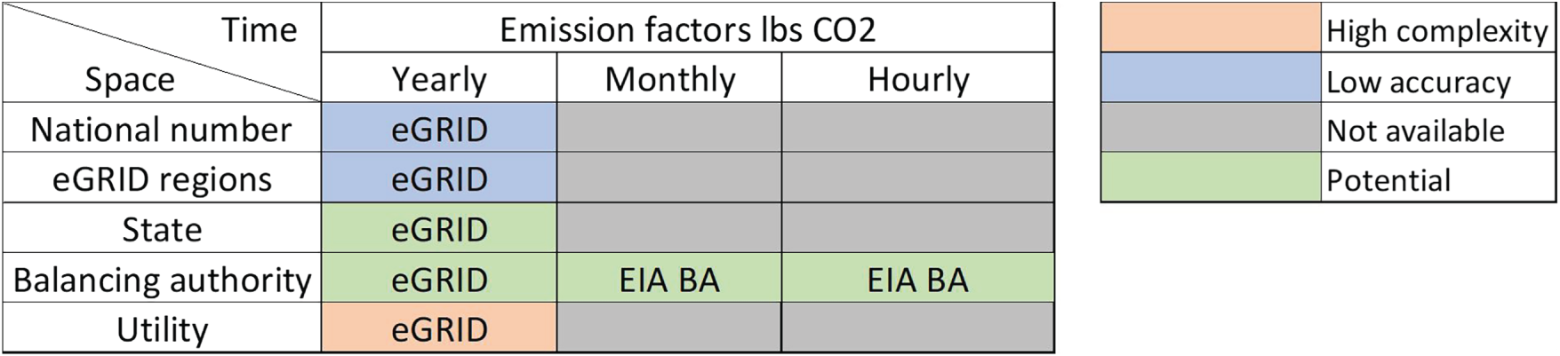
Figure 1: Space and time matrix.

3  Results

The results demonstrate significant spatial and temporal variations in CO2 emission factors, suggesting that a single calculation method is not accurate or efficient in every case. The eGRID data was used to analyze spatial variations.

3.1 Spatial Variation

There is a significant overlap between spatial regions in different categories (e.g., eGRID regions, states, BAs) as shown in Fig. 2. Most BAs are spatially smaller than states and eGRID regions (median number of states and eGRID regions within a BA is 1.0 Table 1). For all 27 eGRID regions and 52 states (including DC and PR), less than 50% have a single balancing authority. 14 states out of 52 have a single balancing authority. 34 out of 67 BAs are contained within a single state and 23 have 2 or 3 neighboring states. Only 3 BAs-PJM, MISO, and SWPP cover a large area, spanning more than 10 states. Fig. 3 shows that when the areas from zipcode polygons corresponding to BAs and states are compared, the majority of BAs are smaller than the states even if they cover parts of 3 states. About 7 out of 67 BAs have larger spatial areas as compared to the states they span.

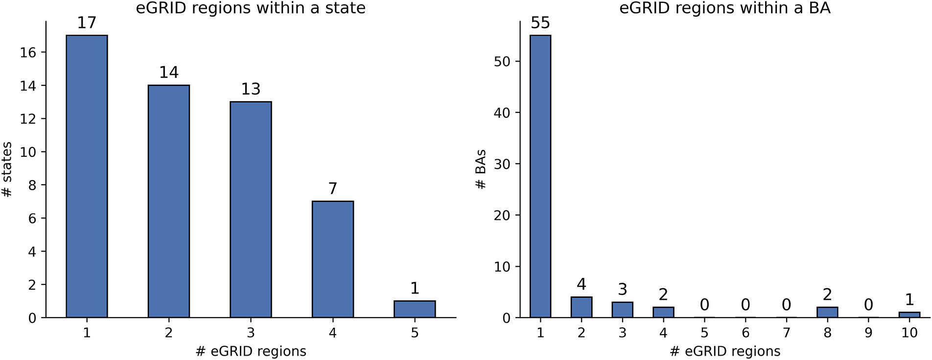
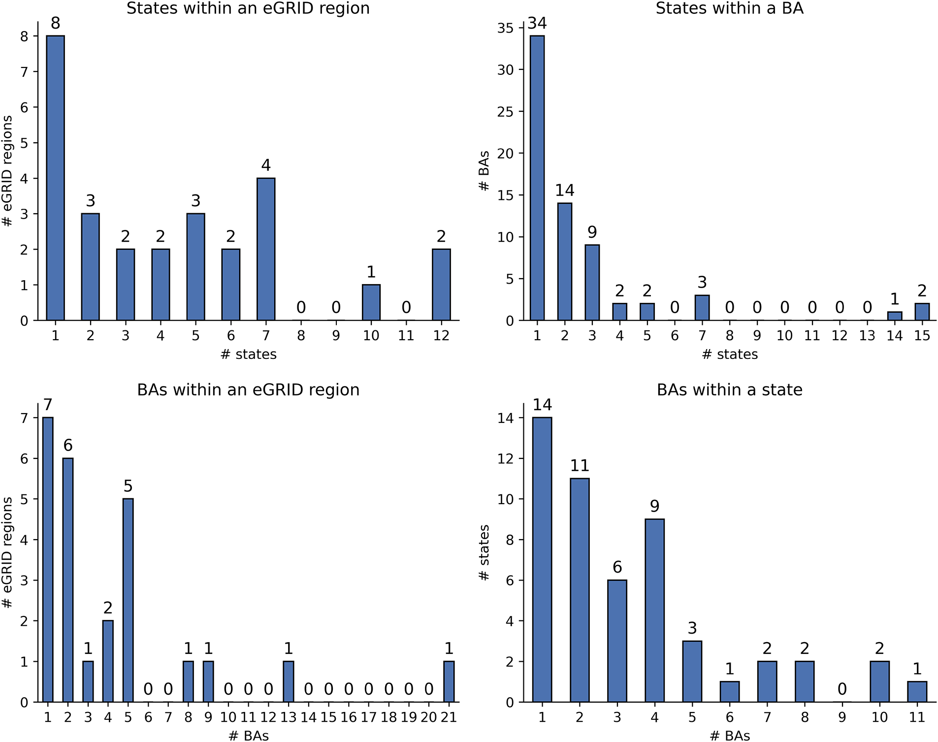
Figure 2: eGRID regions, states, and BAs spatial overlap.

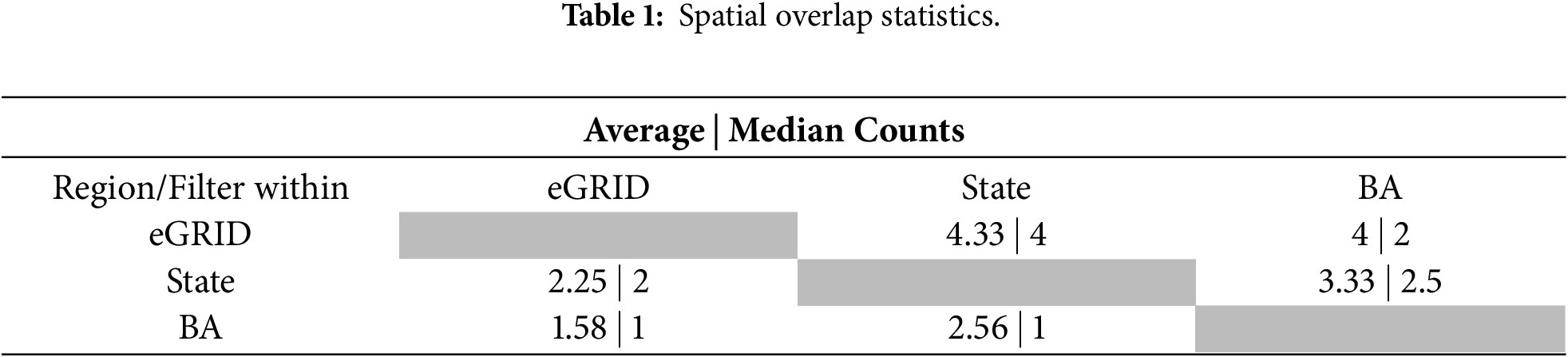
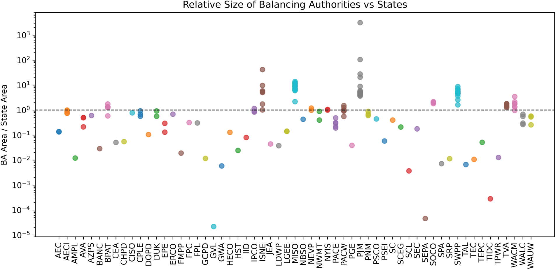
Figure 3: Relative spatial span for BAs and state.

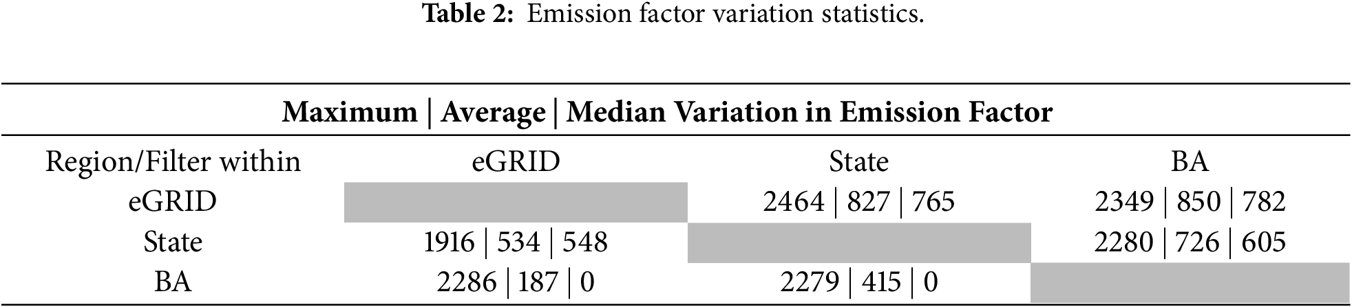
The US national emission factor of 823.15 lbs./MWh is often not representative of particular states. For example, Vermont is 35.63 lbs./MWh, while West Virginia is 1959 lbs./MWh. The emission factor variation among different regions and sub-regions is shown in Fig. 4. This dramatic difference has a clear impact on calculating savings for decarbonization activities. About 50% of the states have an emission factor variation of more than 500 lbs./MWh when considering the eGRID regions or BAs they fall under. For example, in Alabama, the emission factor is 1050 lbs./MWh under SOCO but only 152 lbs./MWh under TVA. About 30% of BAs have a variation of more than 500 lbs./MWh when considering the different states they cover. For example, within PJM, the emission factor is 455 lbs./MWh in New Jersey but 1156 lbs./MWh in Ohio. The maximum variation in emission factors is over 2000 lbs./MWh for all filters (eGRID, State, BA). As can be seen in the metrics (Table 2), the median variation for BAs is 0, since most BAs have a single state or eGRID region. The median and average variations for states and eGRID regions are close, indicating a uniform distribution of emission factor variation.

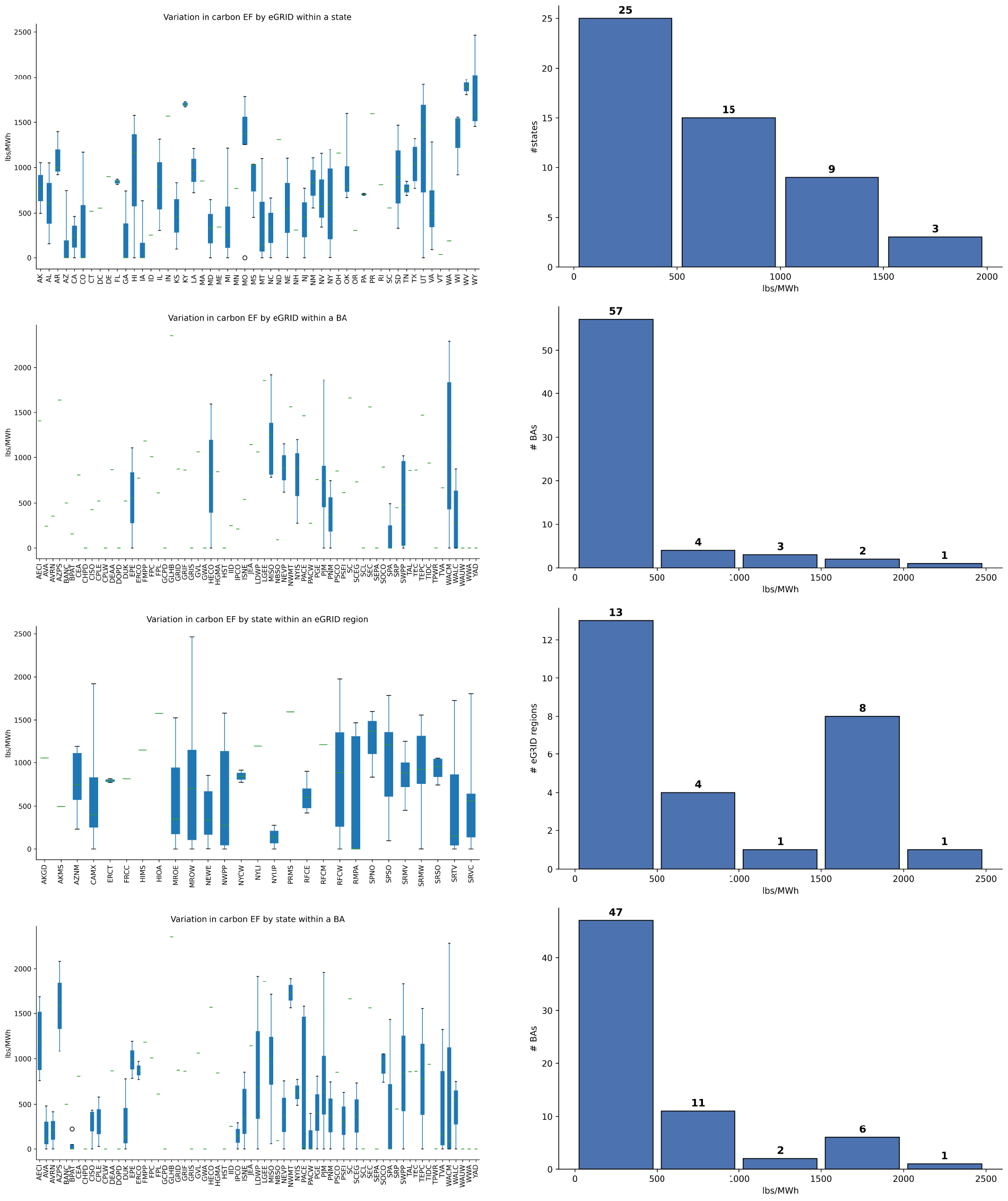
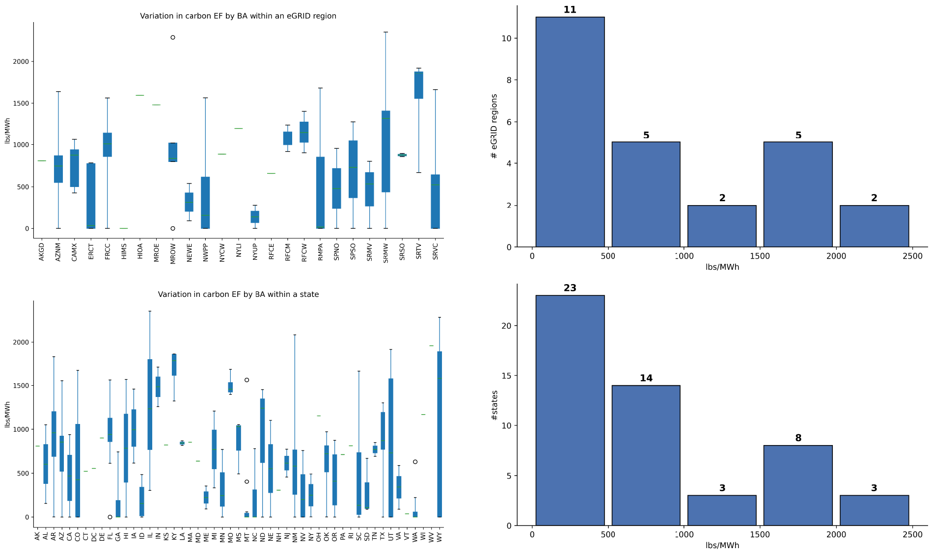
Figure 4: Variation in emission factors (lbs./MWH).

The calculation of utility-level emission factors is classified as “High complexity” in the matrix Fig. 1. This is because of limited or complete data unavailability such as—the service areas of utilities, the interchange of electricity between utilities within a BA and marginal flows. eGRID data is insufficient because it is limited to power plants owned by utilities, omitting information on Power Purchase Agreements (PPAs) and utilities that purchase electricity wholesale (e.g., municipal, local, and rural cooperatives). Some of the utilities mentioned in the eGRID dataset are operators of the power plants and do not provide electricity as retail or wholesale, but have PPAs with distribution level utilities (e.g., Agua Caliente Solar [21]). There are 5106 utilities in the eGRID data, and analyzing them on an individual case basis (to track PPAs, for instance) is complicated. An ideal dataset from utility companies—one similar to EIA’s BA data that considers interchange, would make the hourly emission factor calculation simple.

3.2 Yearly Temporal Variation

The EIA’s BA data was used to analyze temporal variations in emission factors. Analysis of EIA BA data over five years Fig. A1 shows how emission factors change as a result of shifts in utility generation technology and new capital investments. Most balancing authorities reduced their carbon footprint between 2019 and 2023 as can be seen from Fig. 5. For example, PacifiCorp West (PACW) dropped from 808 lbs./MWh to 291 lbs./MWh (a drop of over 500 lbs./MWh) and Gainesville Regional Utilities (GVL) dropped from 1,187 lbs./MWh to 728 lbs./MWh.

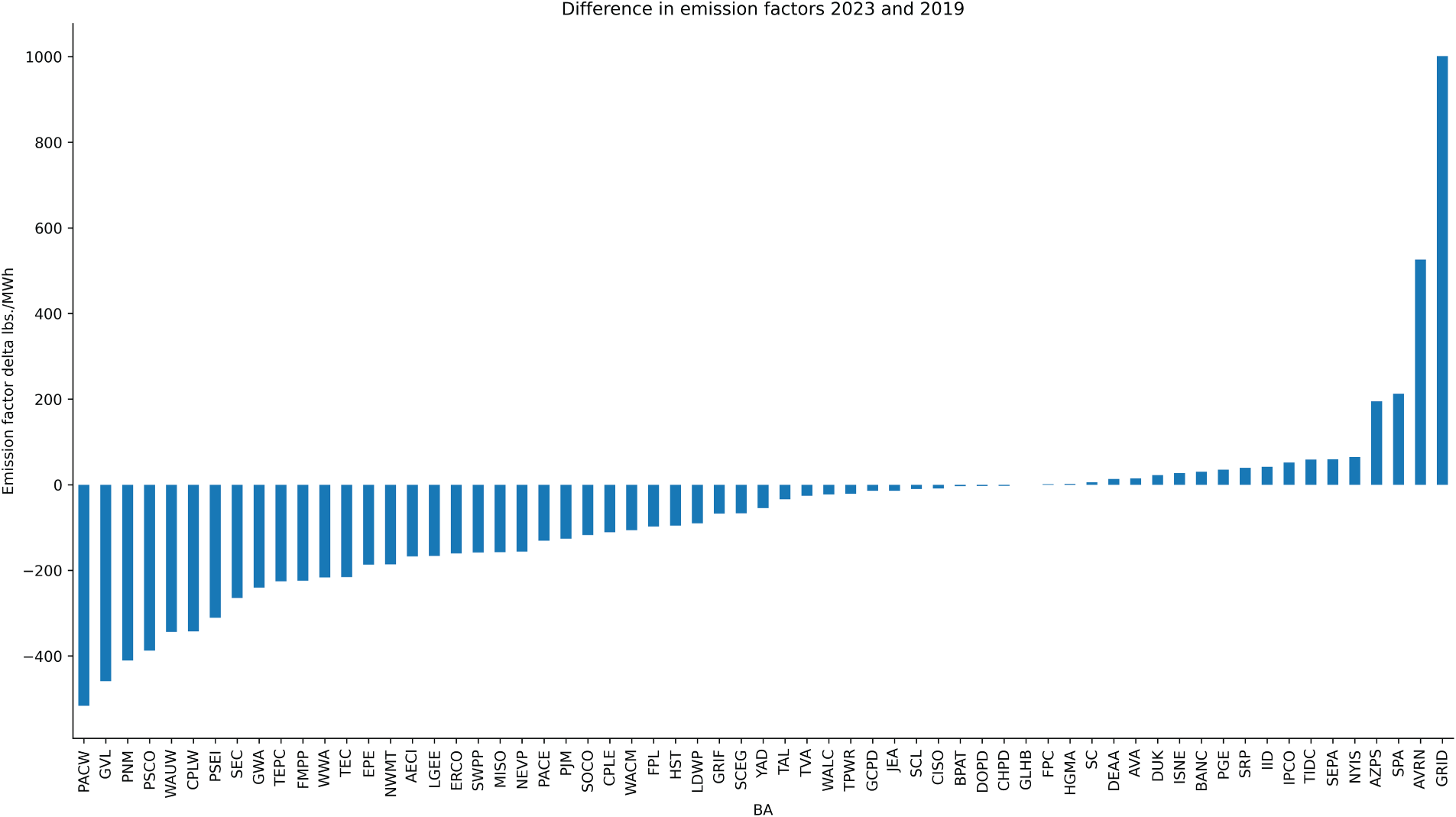
Figure 5: Yearly emission factor variation by balancing authorities.

3.3 Hourly Temporal Variation

Hourly resolution is important when a BA has cleaner and dirtier periods of generation (e.g., solar PV during daytime). The variation between balancing authority’s hourly emission factors is evaluated by calculating the difference between maximum and minimum hourly emission factors as shown in Fig. 6. The average variation between the maximum and minimum hourly emission factors across all balancing authorities is 190 lbs./MWh throughout the day, which is 23% of the national annual average. LDWP, SEPA, and GWA show a high variation of more than 500 lbs./MWh (61% of the national annual average). CHPD, DOPD, TVA, CPLW, LGEE, GCPD, PJM, and GLHB show a low variation of less than 50 lbs./MWh (6% of the national annual average).

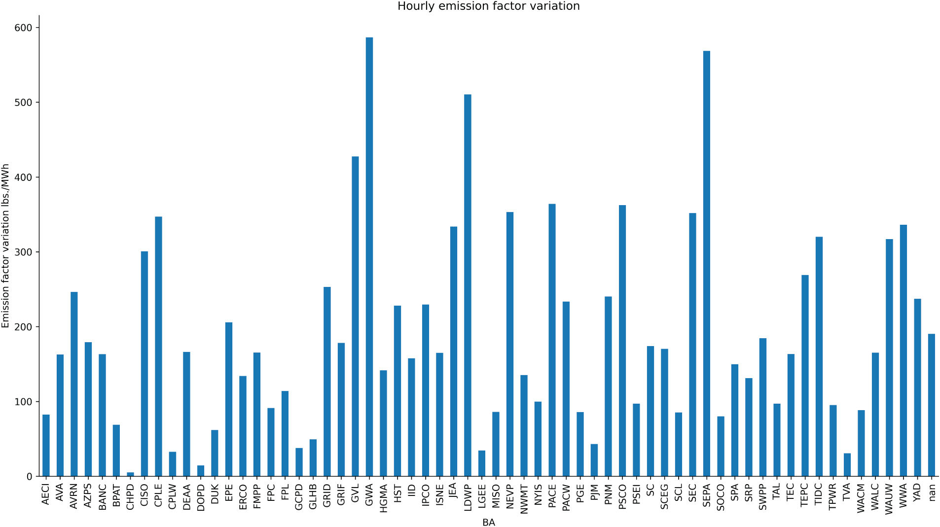
Figure 6: Hourly emission factor variation by BA.

Hourly accounting is necessary because the difference between hourly and yearly emissions depends on the facility’s load profile relative to the BA’s generation curve. 5-min electrical interval data for 25 industrial buildings was obtained from this open-source data “ENERNOC 2012 Commercial Energy Consumption Data” [22] and the emissions were calculated using hourly and annual emission factors. These two cases stood out (Site 674 and 697) where the difference in emission rates calculated by hourly and yearly methods varied by about 10% as shown in Table 3. The detailed list is shown in Appendix B and Table A1.

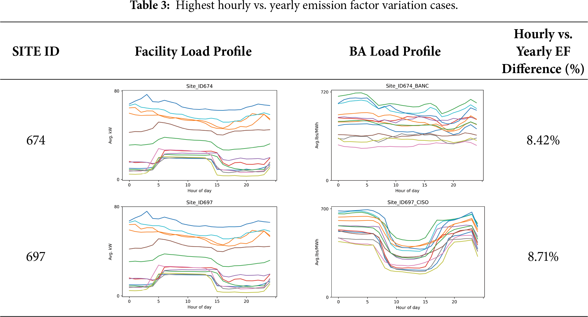
•   Case 1 (Plant 1): Emissions difference of 8% (about 10,000 lbs./year). Consumption was high and constant during September, October, and November (average 44,000 kWh) compared to other months (17,000 kWh). During these high-consumption months, the BA (BANC) generation was also dirtier (550 lbs./MWh average vs. 400 lbs./MWh in other months).

•   Case 2 (Plant 2): Emissions difference of 9% (about 11,000 lbs./year). The plant’s operation curve shows it starts between 3–4 AM and continues until 3–4 PM. The emission rates for this BA are generally lower from 9 AM to 5 PM.

Miller et al. (2022) [23] conducted a similar study by using load profiles of 113,000 simulated residential and commercial buildings and the balancing authorities’ hourly emissions factor profile and found that the average yearly carbon emissions can be over- or under-estimated by 35%. Schäfer et al. [24] found 3.8% reduction in emissions estimation by using higher temporal resolution data.

Further a dataset of hourly loads for eight simulated typical industrial buildings developed by [20] in 2020 was used to calculate the difference between hourly and yearly emission factors. These buildings were ran against all BAs and the temporal difference in emission factors was calculated as shown in Fig. 7. The load profile is shown in Table 4. Periods of cleaner and dirtier production of electricity vary across different BAs. Conducting the analysis across all BAs with the same client load profiles verified the hypothesis that hourly emission factors play a significant role in calculating the carbon footprint. About seven BAs had very high difference between the hourly and yearly emission factors across all eight sites. Other balancing authorities based on the periods of production and consumption by the sites had varying emission factors. This highlights the significance of temporal data to get accurate carbon footprint.

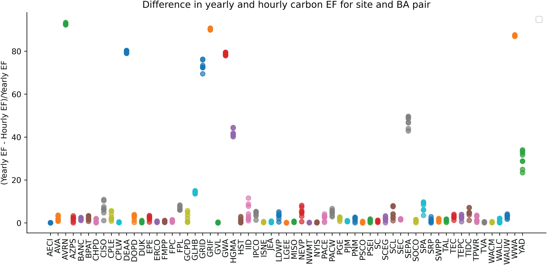
Figure 7: Hourly vs yearly emission factor variation by BA.

4  Discussion

It can be seen from the analysis above that improvements in carbon accounting with higher spatial and temporal granularity are warranted, though they will not be sufficiently accurate in every case. Using data with higher granularity provides significantly improved accuracy over the national average. Parsing the eGRID database by state, eGRID regions, and balancing authority (i.e., power pools) provides higher spatial granularity for more accurate carbon footprint calculations and parsing the EIA hourly electric grid monitoring data provides higher temporal granularity. In addition the EIA data takes into account electricity interchange. Improvements compared to using the national average is significant (e.g., 35.63 lbs./MWh for Vermont vs. 1959 lbs./MWh for West Virginia). Such dramatic differences will have an impact on calculating savings for these local decarbonization activities or on paybacks for importing green power.

Electricity transmission plays a critical role in shaping the spatial allocation of electricity related carbon emissions. Because electricity is frequently generated in one region and consumed in another, the location of emissions does not necessarily coincide with the location of electricity use. Consequently, regions with substantial electricity imports may exhibit consumption related carbon intensities that differ from their local generation based values, while exporting regions may appear less carbon intensive despite hosting carbon intensive generation. Li et al. [25] demonstrated that large scale inter-regional transmission can result in substantial carbon transfers between regions, significantly influencing spatial carbon accounting outcomes. These findings reinforce that carbon accounting approaches based solely on local or annual average emission factors may overlook the effects of transmission. Using state-level data is the simplest and most accessible improvement, a protocol used by tools like the UC-Davis/LBNL suite. However, many states have multiple BAs with different fuel mixes. Using only data from balancing authorities has a similar drawback—PJM, MISO and SWPP cover broad geographic regions with a wide range of carbon emissions, whereas Florida and Montana have 10 different balancing authorities and Washington has 11 in a single state. Utility scale data would help improve the granularity of these broader balancing authorities. In addition energy exchange between utilities would be a great data point that would account for transmission related factors. If a facility wants to understand where the electrons are coming from then a logical path would be to trace the least resistance transmission line. This is where marginal data and transmission maps can be used to figure out which stations have the least load at a given time and based on geographical proximity are most likely to deliver electricity. This would be a huge step towards accurate location based carbon accounting.

Temporal granularity comes in two perspectives. First looking at changes in fuel mixes at one location over several years, which considers, for example, of the transition away from coal and increases in natural gas and renewables. The second way temporal granularity can be important is with seasonal or daily variations in fuel/generator mix at power plants. Daylight hours could see very small emissions which jump up again at night when solar is not available. Seasonal variations of solar and wind availability can also be important. Depending on the balancing authority and facility load profile inclusion of time-of-use carbon emissions is warranted.

A “smart” carbon calculator, which factors in data from power pools, state reports and utilities, can significantly improve accuracy with reasonable effort resulting in better carbon footprint calculations that are needed for credible sustainability planning. A smart carbon calculator with the following characteristics is recommended to provide more accurate carbon accounting.

•   Avoid using the national average emissions factor-most inaccurate

•   The first step to improving accuracy is using eGRID regions and subregions and assume the electricity generated in a region/subregion is consumed within that region/subregion. These boundaries were chosen to represent areas where the majority of electricity generated is consumed locally.

•   States and BAs in most cases are spatially smaller than eGRID regions. State emission factors that come from US EPA’s eGRID do not take into account energy flow between states. However, the EIA’s BA data considers electricity exchange. In cases where BA is spatially smaller than the state, use the EIA’s BA hourly data since it’s more spatially and temporally granular.

•   For large BAs, like the regional transmission organizations (RTO) (e.g., PJM and MISO), where transmission map data and hourly marginal intensities are available, use a model based on electricity flow through the least resistance path.

•   Ideally, but not available now, local utilities would provide coverage maps and hourly input and output data similar to what BAs provide now.

5  Conclusion

This study identifies limitations to available scope 2 carbon emissions intensity data and recommends an approach (“Smart carbon meter”) to improve carbon accounting accuracy. This will have a huge impact on calculating savings for local decarbonization activities and on paybacks for importing green power, important for achieving carbon neutrality.

The novel contributions of the paper include:

Analyses

•   Quantified spatial overlaps between various regions and subregions (Fig. 2 and Table 1).

•   Analysis comparing accuracy of hourly vs. annual emission factors that emphasize the importance of temporal granularity (Table 3 and Fig. 6).

•   Analysis of typical building load curves in different balancing authorities to highlight how hourly consumption affects carbon accounting (Fig. 7).

Guides

•   Practical selection guide for more spatially granular regions using zip code mapping (Fig. 3).

•   Smart carbon calculator tool recommendations

The limitations of this study are

•   Downsizing big BAs to find emission factors for subregions or regional utilities is described qualitatively.

•   For zipcodes on the regional boundary, the actual BA maybe different for the entirety or part of the zip area than the one given by the US DOE tool since the tool gives the most likely BAs associated with a zipcode. The uncertainty analysis for such cases is not conducted.

•   eGRID 2022 data is used, however the analysis can be reproduced for more recent eGRID 2024 data expected by January 2026.

Acknowledgement: The authors acknowledge the support of Rutgers, The State University of New Jersey.

Funding Statement: The authors received no specific funding for this study.

Author Contributions: The authors confirm contribution to the paper as follows: Conceptualization, Aditya Mairal, Todd Rossi and Michael Muller; methodology, Aditya Mairal; software, Aditya Mairal; validation, Aditya Mairal, Todd Rossi and Michael Muller; formal analysis, Aditya Mairal; data curation, Aditya Mairal; writing—original draft preparation, Aditya Mairal; writing—review and editing, Todd Rossi and Michael Muller; visualization, Aditya Mairal; supervision, Todd Rossi and Michael Muller; project administration, Todd Rossi and Michael Muller. All authors reviewed and approved the final version of the manuscript.

Availability of Data and Materials: The authors confirm that the data supporting the findings of this study are available within the article.

Ethics Approval: Not applicable.

Conflicts of Interest: The authors declare no conflicts of interest.

Appendix A BA Yearly Temporal Variation

Figure A1: BA 2019 to 2023 emission factor variation.

Appendix B Hourly Temporal Variation Effect on Emission Factors

References

1. UNFCCC. Paris agreement [Internet]. United Nations. [cited 2015 Dec 23]. Available from: https://unfccc.int/sites/default/files/english_paris_agreement.pdf. [Google Scholar]

2. Stein T. No sign of greenhouse gases increases slowing in 2023-NOAA Research [Internet]. NOAA Research. 2024 [cited 2026 Jan 19]. Available from: https://research.noaa.gov/2024-04-05/no-sign-of-greenhouse-gases-increases-slowing-in-2023. [Google Scholar]

3. Carbon Neutrality by 2045-Office of Planning and Research [Internet]. opr.ca.gov. [cited 2026 Jan 19]. Available from: https://opr.ca.gov/climate/carbon-neutrality.html. [Google Scholar]

4. Apple Newsroom. Apple commits to be 100 percent carbon neutral for its supply chain and products by 2030 [Internet]. Apple Newsroom. 2020 [cited 2026 Jan 19]. Available from: https://www.apple.com/newsroom/2020/07/apple-commits-to-be-100-percent-carbon-neutral-for-its-supply-chain-and-products-by-2030/. [Google Scholar]

5. Google. Aiming to Achieve Net-Zero Emissions-Google Sustainability [Internet]. Google Sustainability. 2023 [cited 2026 Jan 19]. Available from:https://sustainability.google/operating-sustainably/net-zero-carbon/. [Google Scholar]

6. Smith B. Microsoft will be carbon negative by 2030 [Internet]. Official Microsoft Blog. Microsoft. 2020 [cited 2026 Jan 19]. Available from: https://blogs.microsoft.com/blog/2020/01/16/microsoft-will-be-carbon-negative-by-2030/. [Google Scholar]

7. US EPA O. Greenhouse Gases at EPA [Internet]. US EPA. 2015 [cited 2026 Jan 19]. Available from: https://www.epa.gov/greeningepa/greenhouse-gases-epa. [Google Scholar]

8. Scope 2 Guidance—GHG Protocol [Internet]. ghgprotocol.org. [cited 2026 Jan 19]. Available from: https://ghgprotocol.org/sites/default/files/2023-03/Scope2Guidance.pdf. [Google Scholar]

9. FST [Internet]. Lbl.gov. 2026 [cited 2026 Jan 19]. Available from: https://industrialdecarb.lbl.gov/apps/fst/. [Google Scholar]

10. LCC [Internet]. Lbl.gov. 2026 [cited 2026 Jan 19]. Available from: https://industrialdecarb.lbl.gov/apps/lcc/. [Google Scholar]

11. de Chalendar JA, Taggart J, Benson SM. Tracking emissions in the US electricity system. Proc Nat Acad Sci. 2019;116(51):25497–502. doi:10.1073/pnas.1912950116. [Google Scholar] [PubMed] [CrossRef]

12. Chen L, Wemhoff AP. Predicting embodied carbon emissions from purchased electricity for United States counties. Appl Energy. 2021;292:116898. doi:10.1016/j.apenergy.2021.116898. [Google Scholar] [CrossRef]

13. Gurney KR, Liang J, Patarasuk R, Song Y, Huang J, Roest G. The Vulcan version 3.0 high-resolution fossil fuel CO2 emissions for the United States. J Geophys Res Atmos. 2020;125(19):e2020JD032974. doi:10.1029/2020jd032974. [Google Scholar] [PubMed] [CrossRef]

14. Gurney KR, Dass P, Kato A, Mitra B, Modeste Kameni N. Scope 2 estimates of carbon dioxide emissions from electricity consumption at the US census block group scale. Sci Data. 2024;11(1):1344. doi:10.1038/s41597-024-04180-5. [Google Scholar] [PubMed] [CrossRef]

15. Goldstein B, Gounaridis D, Newell JP. The carbon footprint of household energy use in the United States. Proc Nat Acad Sci. 2020;117(32):19122–30. doi:10.1073/pnas.1922205117. [Google Scholar] [PubMed] [CrossRef]

16. US EPA O. Data Explorer [Internet]. US EPA. 2020 [cited 2026 Jan 19]. Available from: https://www.epa.gov/egrid/data-explorer. [Google Scholar]

17. Real-time Operating Grid-U.S. Energy Information Administration (EIA) [Internet]. [cited 2026 Jan 19]. Available from: https://www.eia.gov/electricity/gridmonitor/dashboard/electric_overview/US48/US48. [Google Scholar]

18. The emissions & generation resource integrated database eGRID technical guide with year 2022 data clean air markets division [Internet]. 2022 [cited 2026 Jan 19]. Available from: https://www.epa.gov/system/files/documents/2024-01/egrid2022_technical_guide.pdf. [Google Scholar]

19. Energy.gov. 2026 [cited 2026 Jan 19]. Available from: https://www.energy.gov/sites/default/files/2023-11/BalancingAuthorityLookupTool.xlsx. [Google Scholar]

20. Angizeh F, Ghofrani A, Jafari MA. Dataset on Hourly Load Profiles for a set of 24 facilities from industrial, commercial, and residential end-use sectors. Mendeley Data. 10.17632/rfnp2d3kjp.1.2020. [Google Scholar] [CrossRef]

21. Clearway Energy. Clearway energy, Inc. Investor presentation [Internet]. 2023. [cited 2026 Jan 19]. Available from: https://investor.clearwayenergy.com/static-files/71838dcc-db51-4e13-ac43-a07e403d5691. [Google Scholar]

22. ENERNOC 2012 commercial energy consumption data. Github.io. 2026 [cited 2026 Jan 19]. Available from: https://trynthink.github.io/buildingsdatasets/show.html?title_id=enernoc-2012-commercial-energy-consumption-data. [Google Scholar]

23. Miller GJ, Novan K, Jenn A. Hourly accounting of carbon emissions from electricity consumption. Environ Res Lett. 2022;17(4):044073. doi:10.1088/1748-9326/ac6147. [Google Scholar] [CrossRef]

24. Schäfer M, Cerdas F, Herrmann C. Towards standardized grid emission factors: methodological insights and best practices. Energy Environ Sci. 2024;17(8):2776–86. doi:10.1039/d3ee04394k. [Google Scholar] [CrossRef]

25. Li Z, Li J, Cao Z, Hu K, Ao R, Li J, et al. Spatiotemporal carbon footprints of electricity production and consumption in China. Cell Rep Sustain. 2025;2(11):100466. doi:10.1016/j.crsus.2025.100466. [Google Scholar] [CrossRef]