
 Login
Login Register
 Submit a Paper
 Propose a Special lssue
 Open Access
ARTICLE

A Data-Driven Method for Rapid Prediction of Polarization Curves in Proton Exchange Membrane Electrolysis Cell
1 Institute for Clean Energy Technology, North China Electric Power University, Beijing, China
2 School of Mathematics and Physics, North China Electric Power University, Beijing, China
* Corresponding Authors: Hao Cheng. Email: ; Yongli Li. Email:
(This article belongs to the Special Issue: Hydrogen Energy Systems: Storage, Power-to-Hydrogen, and AI-Enabled Design, Planning, and Operation)
Energy Engineering 2026, 123(9), 9 https://doi.org/10.32604/ee.2026.082907
Received 25 March 2026; Accepted 08 May 2026; Issue published 06 August 2026
 View Full Text
 Download PDF
Abstract
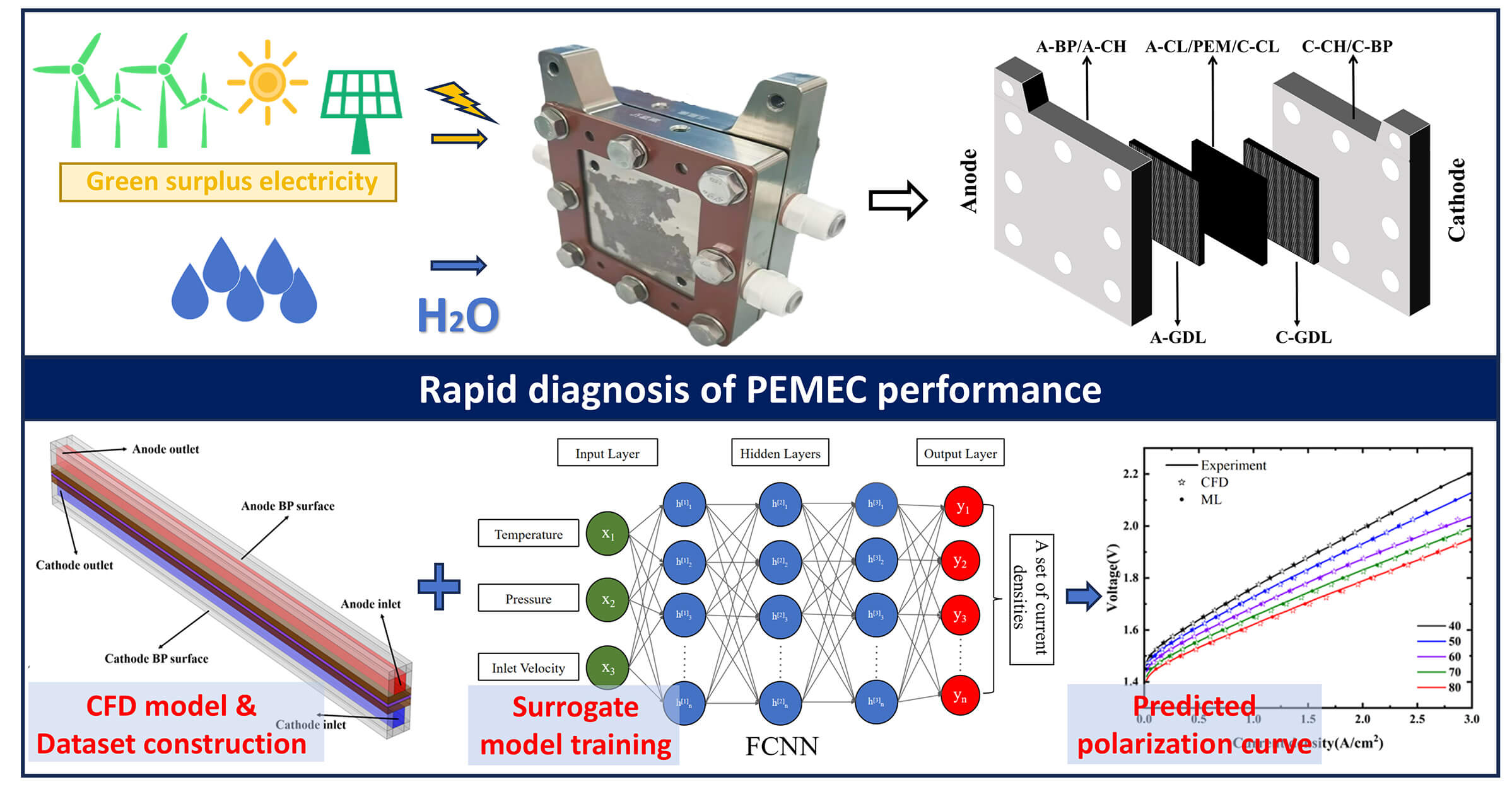
The prediction of the steady-state performance of the electrolysis cell is not only crucial for evaluating the rationality of its design and operational benchmarks, but also provides an important foundation for understanding its dynamic response behavior. This paper presents an efficient data-driven method based on three-dimensional two-phase numerical simulation and machine learning (ML) to rapidly predict the steady-state performance of proton exchange membrane electrolysis cells (PEMEC) under multi-physics field coupling conditions. The framework is based on three key operating parameters—temperature, pressure, and inlet flow velocity. A polarization curve dataset was constructed through multi-condition numerical simulations, and surrogate models were systematically trained using five distinct ML algorithms: random forest (RF), extreme gradient boosting (XGBoost), support vector regression (SVR), gaussian process regression (GPR), and fully connected neural network (FCNN). The results show that the constructed surrogate models can efficiently output complete polarization curves using only operating parameters as inputs. Validation against experimental results confirms that the FCNN performs the best overall prediction performance, achieving high accuracy with prediction errors consistently within ±0.5% of the actual values across the interpolation temperature range, and demonstrating adaptability in extrapolation under varying temperatures. This ML collaborative method is applicable to the rapid performance assessment and analysis of PEMEC and provides valuable insights for operation optimization under extreme conditions.Graphic Abstract
Keywords
Hydrogen energy is widely regarded as one of the key directions for achieving the clean energy transition due to its high energy density and environmental friendliness [1,2]. At present, the supply of hydrogen energy in the market is still dominated by grey hydrogen produced from fossil fuels. The production process is accompanied by a large amount of carbon dioxide, which cannot fundamentally alleviate the pressure of carbon emissions. In contrast, green hydrogen produced via water electrolysis powered by renewable energy sources such as wind and photovoltaic energy generates almost no carbon emissions over its entire life cycle. Moreover, with its high purity and multiple application scenarios, this approach is gradually becoming an ideal route for developing clean hydrogen energy [3,4]. Common water electrolysis technologies for hydrogen production include alkaline water electrolysis (AWE), solid oxide electrolysis (SOE) and proton exchange membrane water electrolysis (PEMWE). The advantages and disadvantages of these three water electrolysis technologies are summarized in Table 1.

However, the large-scale industrial application of current proton exchange membrane electrolysis cell (PEMEC) is severely challenged by its long-term performance degradation and limited service life, arising from the complex coupling of electrical, thermal, and mechanical stresses in a multi-physics environment [11]. Specifically, under high current density and transient overvoltage conditions, the gas production rate at the anode increases sharply, and a large number of bubbles accumulate and clog, which can easily lead to localized heat and mass transfer performance deterioration and uneven current distribution. This causes localized overheating and significant temperature gradients, which results in irreversible damage to key components, including the catalyst layer (CL), gas diffusion layer (GDL), and proton exchange membrane (PEM). More critically, to adapt to the intermittency of renewable energy sources like wind and solar power, electrolysis cells often have to operate over wide load ranges under dynamic conditions. The frequent startup-shutdown cycles and load fluctuations impose continuous mechanical and electrochemical stresses, further accelerating the degradation process and severely limiting the long-term economic viability and reliability of the system [12]. Therefore, establishing standard-condition polarization curves as benchmarks and comparing them with operational data is essential for diagnosing cell health and identifying degradation mechanisms [13]. Furthermore, precise modeling and prediction of PEMEC performance under variable operating conditions provide a foundation for adaptive control strategies and operational optimization, thereby enhancing system performance and long-term reliability [14].
To reveal the complex processes involving multi-physics coupling, predict polarization curves, and analyze performance evolution under varying conditions, computational fluid dynamics (CFD) based numerical simulation has emerged as a widely adopted tool. The CFD method can simulate the coupled the cross-scale and nonlinear interactions between two-phase flow, heat and mass transfer, and electrochemical reactions within the internal structure of the PEMEC, thereby systematically establishing the relationship between its internal physical state and macroscopic performance [15]. For instance, Wang et al. [16] numerically investigated the water distribution and temperature fields by coupling the Butler-Volmer equation with liquid water saturation and temperature variables; Wu et al. [17] established a three-dimensional (3D) multiphase full-cell model using the volume of fluid (VOF) method, incorporating gas–liquid two-phase flow in the flow channels, and systematically investigated the effects of key parameters and structural features through numerical simulations. Zhou et al. [18] systematically investigated the effects of various parameters on heat and mass transfer performance and electrolysis efficiency based on a 3D two-phase model; while Jiang et al. [19] precisely captured the spatial distribution of temperature, gas fraction, and current density, and clarified the mechanism of the impact of two-phase flow on the overall performance by coupling electrochemical and heat and mass transfer models. Additionally, Su et al. [20] numerically compared a novel mesh-like anode channel with a traditional straight-through design and demonstrated its superior performance in promoting oxygen removal and improving current density uniformity. These studies have effectively assessed the physical and chemical processes within the electrolysis cell using numerical simulation methods, providing important support in revealing mechanisms and predicting performance compared to time-consuming and labor-intensive pure experimental methods.
However, the high-density meshing and strongly nonlinear governing equations in CFD multi-physics models often lead to excessive computational costs during multi-parameter optimization and multi-condition comparisons. To address this issue, data-driven ML methods have been adopted in PEMEC studies for rapid modeling and performance prediction, leveraging their strength in handling large-scale, complex datasets [21]. In terms of parameter analysis and mechanism interpretation, existing studies have conducted systematic exploration through data integration and multiple algorithms. Günay et al. [22] integrated data from multiple literatures and adopted methods such as box-plot analysis, principal component analysis, and classification and regression tree to systematically evaluate the influence of multiple parameters on the performance of electrolysis cells. Ding et al. [23] established a database from membrane electrode assembly (MEA) data, employing 9 mainstream ML algorithms to predict the current density and decay rate at a specific voltage, and complemented by a model interpretability analysis using partial dependence plot (PDP) and shapley additive explanations (SHAP). In terms of predictive modeling and optimization, deep learning, with its multi-layer neural network structure, is particularly suitable for fitting complex implicit mapping relationships between inputs and outputs [24]. Siddiqa et al. [25] combined CFD simulation with ML surrogate models to conduct high-precision prediction and parameter correlation analysis of PEMEC performance. Wang et al. [26] utilized the backpropagation neural network and the non-dominated sorting genetic algorithm (NSGA-II) to achieve multi-objective prediction and optimization of PEMEC performance, thereby synergistically enhancing temperature safety, electrochemical reaction rate, and hydrogen evolution. Timurkutluk et al. [27] applied artificial neural networks to the design of the microstructure of solid oxide fuel cell electrodes, with a focus on studying the influence of particle size on the density of the active triple-phase boundary. Their method generated 3D electrode microstructures using the Dream.3D software and utilized artificial neural networks for efficient prediction, significantly improving the design accuracy and efficiency. Overall, compared with traditional experimental and simulation methods, ML has significantly accelerated the parameter research and structural optimization design process of PEMEC.
Despite this, current research still has two main limitations: On the one hand, most studies focus on static performance prediction at specific operating points, lacking the investigation of a wide range relationship between working voltage and current density, resulting in insufficient research on the prediction of the complete polarization curve of electrolysis cells based on operating conditions or structural parameters; On the other hand, in the model evaluation system, most existing studies focus on the extrapolation accuracy of the model within the training range, while often neglecting its extrapolation ability under broader or unseen operating conditions. However, the latter is crucial for practical engineering applications.
To address the above issues, this study proposes a data-driven method that integrates numerical simulation and ML, aiming to achieve efficiency and high-precision prediction of the performance of electrolysis cells under different working conditions. Specifically, the main innovations of this study include the following aspects. A mapping strategy from operating parameters to a complete current density sequence was proposed, which can directly predict the entire polarization curve rather than individual operating points. A systematic comparison was conducted on five machine learning algorithms with different principles, and their interpolation and extrapolation capabilities were comprehensively evaluated. The constructed alternative model only requires the input of three operating parameters (temperature, pressure, and inlet velocity), and can generate a complete polarization curve with high accuracy within seconds, significantly improving the prediction efficiency. The data-driven method developed here demonstrates excellent feasibility in this specific PEMEC configuration. As a proof-of-concept study, this method framework has the potential for further expansion and migration in the future, and is of reference value for performance prediction and design optimization of specific structure electrolysis cells. Fig. 1 summarizes the overall process of this study.

Figure 1: Flowchart of the research process.
2 Physical Model and Numerical Simulation
Fig. 2a,b shows the overall 3D view and XZ cross-sectional view of PEMEC. The entire structure of the PEMEC is centrally symmetrical, with the PEM located at the center and the anode and cathode on both sides, respectively. From the center outward, the layers are the CL, GDL, CH, and the bipolar plate (BP) on both the anode and cathode, respectively. During the operation of the PEMEC, water molecules exist in liquid form. Water enters the PEMEC through the plates on the anode side, and then passes through the GDL to reach the anode catalyst layer, where water molecules undergo an oxygen evolution reaction (OER), losing electrons and being oxidized, thereby generating protons, electrons and oxygen (

Figure 2: (a) PEMEC single channel (b) X-Z cross-section (c) boundary surface.
In practical applications, a PEMEC stack is composed of many parallel single channels. However, considering that its overall channels are arranged periodically and in order to reduce computational costs and achieve higher computational efficiency and cost-effectiveness, the numerical simulation adopts a simplified model of a single flow channel [26]. The fluid flows in from one side of the anode channel, while carrying the

The PEMEC model couples electrochemical reactions, multiphase flow, and heat and mass transfer to simulate the actual operation of the electrolysis cell. The numerical model is established under steady-state conditions and is based on the following key assumptions [28–30]:
(1) Reactant water and gas are treated as ideal compressible flowing fluids;
(2) The flow operates at low Reynolds numbers and is laminar;
(3) The effects of gravity, contact thermal resistance and contact resistance are negligible;
(4) The materials of catalyst layer and gas diffusion layer are homogeneous and isotropic porous media;
(5) The permeation of
(6) The water remains in the liquid phase without phase change.
(1) Mass transport equation
The continuity equation of liquid water in CL, GDL and CH of cathode and anode is given by the following formula:
where
The Brinkman equation extended on the basis of Darcy’s law is particularly suitable for simulating fluid flow in porous media. The momentum conservation equation at the core is given by the following formula [13,28]:
where
The corresponding gas continuity equation, momentum equation and viscous shear stress of gas are given as follows:
where
In porous media of GDL and Cl, capillary pressure is an indispensable driving force for fluid flow, and it is also an important link between gas-liquid two-phase fluids. Capillary pressure can be expressed as [31]:
where
where
where
According to Fick’s law [31], the material conservation equation in the cathode and anode is as follows:
where
(2) Energy transport equation
The energy equation in the calculation area of the model can be expressed as:
where
where
(3) Charge transport equation
According to Ohm’s law, the charge conservation equation of electrons and protons is given by the following formulas [26]:
where
The electrochemical reactions in the cathode and anode are expressed by the modified Butler-Volmer (B-V) equation [33]:
where
where
The formulas for calculating the exchange current densities
where

Table 4 presents the boundary condition settings adopted in the model. The surface of the anode plate is set as adiabatic and has a potential condition, while the surface of the cathode plate is also made to be adiabatic but has potential is 0. The left and right walls of the electrolysis cell are defined as symmetrical boundaries. The remaining boundary surfaces of the electrolysis cell are set as solid walls and are regarded as insulating and electrically insulated boundaries. During the operation of the electrolysis cell, the fluid enters the entire system at a constant superficial velocity and temperature through the surfaces of the anode inlets. The anode and cathode outlets are set as constant pressure outlets, and in the flow and heat transfer models, the outlets are commonly set as free outlets. Fig. 2c shows the 3D model along with the corresponding boundary positions and names.

2.3 Grid Independence Verification
The numerical simulation is carried out on a computer equipped with an AMD EPYC 7J13 64-Core Processor and 256 GB of memory. In this study, the finite element method in CFD is used to calculate the steady-state process and solve the fully coupled mathematical equations. The sparse matrix solver PARDISO is used to solve each physical field variable. The variable residuals of each solution step are constrained, and the relative tolerance is set to 1 × 10⁻⁵. A structured grid is adopted for the computational domain, with the grid cells being hexahedral grids. Considering that the size range of different components in the electrolysis cell is relatively large, different grid sizes are used in different areas for spatial discretization. The catalyst layer in particular is not only the main site of electrochemical reactions, but also much thinner than other components. Therefore, a finer grid division is adopted to effectively capture heat and mass transfer as well as electrochemical characteristics. The number of grids in PEM, GDL and CH is at a medium level, while the BP region adopts a relatively sparse grid division method. The grid division results are shown in Fig. 3a,b. Meanwhile, in order to avoid calculation errors caused by grid division, the grid independence is verified under the condition of constant working operating parameters. The working operating parameters are set as follows: (1) Voltage: 1.675 V; (2) Temperature: 60°C (3) Pressure: 1 atm; (4) Inlet velocity: 0.05 m/s. Adjust the number of mesh cells in the 3D model to study the influence of mesh cell variations on current density. The number of grid cells ranges across 5 groups, namely 12,040, 18,060, 24,080, 30,100 and 36,120. The current density and calculation time corresponding to different grid cell counts are shown in Fig. 3c. After balancing the computational accuracy and the computational cost, a grid count of 24,080 is adopted to ensure grid independence and high computational efficiency.

Figure 3: (a) Grid diagram 3D view (b) X-Z cross-section (c) grid independence test.
To ensure the accuracy of the model, the performance of the electrolysis cell at different temperatures was evaluated through numerical simulation, and the polarization curves obtained from the numerical simulation were compared with the experimental data. In the electrolysis cell used in the experiment, the membrane electrode is a commercial product. The proton exchange membrane is Nafion115, the anode catalyst is IrO2 with a loading of 2.0 mg/cm2, and the cathode catalyst is Pt/C with a loading of 1.0 mg/cm2. Both the anode and cathode diffusion layers are titanium felt. The porosity of the anode is 56% and that of the cathode is 78%. The plate is made of pure titanium material and has corresponding flow field structure inside, including 15 parallel flow channels with length of 30 mm, width of 0.75 mm, depth of 1 mm and rib width of 0.75 mm. Before measuring the polarization curve, the catalyst was activated by flowing deionized water into the electrolysis cell at a certain flow rate for 1 h. The temperature of the electrolysis cell was set at 60°C. Then, the electrolysis was carried out continuously at a current density of 1 A/cm2 for 1 h. After the activation was completed, the polarization curve was collected using the step current method. The current density range was set from 0 to 3 A/cm2, with a total of 40 measurement points. Each current density was maintained for 4 min, with an interval of 10 s, and the voltage average value in the last 2 min was taken as the recorded data for that point.
The experimental test system is shown in Fig. 4, and the comparison between the results obtained from numerical simulation and the experimental data is shown in Fig. 5. The dimensions of the geometric structure, boundary conditions and parameter settings in the simulation are consistent with those in the experiment. A single-channel model was used for the calculations. Symmetrical conditions were applied at both sides of the wall, and the anode inlet velocity was set at 0.074 m/s. In Fig. 5a, all the scattered data are obtained from experimental tests. In Fig. 5b, the curves are fitted to the experimental data in Fig. 5a, and the scattered data points correspond to the numerical simulation results. It can be seen from the figure that the simulation results obtained by the numerical model are basically consistent with the experimental data. This proves the reliability and accuracy of the model in predicting the performance of the electrolysis cell.

Figure 4: Test rig for characterizing polarization curves of PEMEC under various operating conditions. (a) Schematic view; (b) photo view.

Figure 5: Comparison of numerical simulation and experimental results at different temperatures (a) experimental data (b) numerical simulation (curves) and experimental data (scattered points).
The reliability of surrogate models trained through ML largely depends on the dataset collected. The multi-physics PEMEC model verified by grid independence and experimental data was used as the framework for generating training data. Moreover, a total of three operating parameters were considered, including temperature, pressure and inlet velocity, to explore the sensitivity of the polarization curve of the electrolysis cell to these parameters. To ensure that the sampling points did not repeat and were evenly distributed in the 3D space corresponding to these parameters, the Latin Hypercube Sampling was chosen. This method is a statistical approach for multi-dimensional parameter space sampling and is widely applied in fields such as uncertainty quantification, sensitivity, and engineering simulation [35]. Table 5 lists the sampling ranges corresponding to each variable. During the data generation process, for each set of sampling operating condition parameter combinations (temperature, pressure, inlet velocity), using the numerical model within a fixed voltage range (1.475–2.025 V), the corresponding current density was calculated with a step size of 0.025 V, thereby obtaining a complete polarization curve composed of discrete points. Based on this, the constructed dataset defines each sample as a tuple consisting of three operational conditions, and it is associated with a 24-dimensional current density vector calculated at 24 pre-defined equally spaced voltage points. A total of 1024 sets of data were obtained, each set containing three operating parameters and the corresponding polarization curves. The polarization curves were calculated by simulating different voltage values with a constant set step size to obtain current values. Each set of polarization curves contains 24 current values. During the training process, 80% of the data were selected as the training set, while the remaining 20% were split in a 1:1 ratio into the validation set and the test set to evaluate the error and accuracy of the ML model.

3.2 Data Preprocessing and Model Evaluation
Because the selected operating parameters and polarization curve data span different value ranges with significant order-of-magnitude differences, min–max normalization is applied in this study to eliminate scale effects and ensure consistent feature contributions [36]. Meanwhile, reverse normalization is performed on the model outputs to obtain the actual predicted current density for comparison with the original data. For each data point x corresponding to the normalized
where,
The training and testing of the ML surrogate models were carried out on a Windows PC, the CPU is AMD EPYC 7J13 64-Core Processor and the GPU is NVIDIA GeForce RTX 4090. The ML algorithm is implemented in the virtual environment established by Anaconda, using Python 3.11.7 Scikit-learn 1.4.2 and Pytorch 2.6.0, with the corresponding CUDA version being 12.6. To evaluate the predictive ability of the model, three evaluation metrics were adopted to gain a more comprehensive understanding of the model’s predictive performance, namely the R-square (R2), root mean square error (RMSE), and mean absolute percentage error (MAPE) [37–39]. The calculation formulas for evaluation metrics are as follows:
where
This study employed five different ML algorithms, namely random forest (RF), extreme gradient boosting (XGBoost), support vector regression (SVR), gaussian process regression (GPR), and FCNN. By comparing and analyzing the evaluation indicators, a more comprehensive understanding of the algorithm model can be achieved, and the potential of each algorithm can be quantified for subsequent predictions and comparisons with experimental data. The following section briefly discusses the differences and characteristics of these ML algorithms.
Both RF and XGBoost belong to the ensemble learning paradigms based on decision trees, but their core concepts and implementation paths are completely different. The brief algorithm schematic diagram is shown in Fig. 6. RF adopts the Bagging idea, enhancing model performance by constructing a large number of independent decision trees and integrating their results. The core lies in introducing dual randomness, namely the random sampling with replacement of training samples and the random selection of features during node splitting, to ensure the differences between trees and effectively reduce the risk of overfitting. XGBoost follows the Boosting idea, serially constructing a series of trees in a forward step-by-step manner. Each new tree focuses on learning and correcting the residuals or prediction errors of the previous tree. It controls the model complexity by introducing a regularization term into the objective function and uses the loss function for efficient optimization [22,40,41].

Figure 6: Schematic diagram of ensemble learning based on decision trees.
SVR and GPR are both powerful nonlinear regression methods based on kernel techniques, which are particularly suitable for data with small sample sizes, high dimensionality and complex patterns. However, they offer different modeling perspectives. The core objective of SVR is to find a fitting function that can make the majority of the samples fall within the
FCNN is composed of an input layer, several hidden layers and an output layer. All neurons between the layers are connected in pairs, as shown in Fig. 7. The core capability of this model lies in automatically learning highly complex and nonlinear mapping relationships from the original input to the target output through cascading linear transformations and nonlinear activation functions. However, this powerful capability also brings about a distinct “black box” characteristic, making the model’s decision-making process difficult to explain. Meanwhile, it usually requires large-scale training data support to avoid falling into overfitting [25,26,28]. In this study, the hidden layers of the neural network were set to 3 layers, with the number of neurons in each layer being 32, 64, and 32, respectively. The activation function used was ReLU, and the optimizer employed was Adam with weight decay. On this basis, grid search optimization was conducted for hyperparameters such as learning rate, batch size, and weight decay coefficient. Finally, the learning rate was determined to be 0.001, the batch size to be 256, and the weight decay coefficient to be 0.01. Based on this configuration, subsequent research was carried out.

Figure 7: Schematic diagram of a fully connected neural network.
4.1 Numerical Simulation Results
The middle XZ cross-section temperature distribution in the electrolysis cell under different voltages is shown in Fig. 8. As can be seen from the figure, at voltages of 1.50 and 1.75 V, the inlet water flow with a higher temperature on the anode side results in the average anode temperature being significantly higher than that on the cathode side. The temperature distribution of the XZ cross-section shows a continuous downward trend from the anode flow channel to the cathode flow channel. However, as the voltage is increased to 2 V, the anode temperature becomes lower than that of the cathode. This is because the ohmic heat generated by the conductive medium due to high voltage is much greater than the heat required for the chemical reaction, resulting in the temperature of the central film being higher than that on both sides of the cathode and anode. Meanwhile, in addition to participating in chemical reactions, liquid water serves as an important heat transfer medium. Flowing liquid water carries away a large amount of heat, resulting in a lower overall temperature of the anode compared with the cathode side. The velocity distribution of section XZ at different positions along the Y-axis is shown in Fig. 9. The water flow velocity at the anode side inlet is a constant value, while the cathode side inlet does not allow water to pass through. Only a portion of the water seeps through the membrane to reach the cathode. Under the influence of boundary conditions and fluid viscosity, the velocities at the centers of the anode and cathode are significantly higher than those in the surrounding wall areas, while the velocity distribution of the XZ section at three different positions on the anode side is similar. At the cathode, due to the penetration of water on the anode side and the generation of

Figure 8: Temperature distribution in the middle XZ cross-section of PEMEC at various voltages.

Figure 9: Velocity distribution in XZ cross-section of PEMEC at different positions.

Figure 10: Distribution of the middle XY cross-section of PEMEC (a) Temperature (K) (b) current density (A/cm2) (c) electrolyte conductivity (S/m).
In Figs. 11–14, a comprehensive 3D distribution image of temperature,

Figure 11: 3D distribution of temperature in PEMEC under various voltages.

Figure 12: 3D distribution of

Figure 13: 3D distribution of

Figure 14: 3D distribution of
4.2 Performance Comparison of ML Algorithms
Firstly, the prediction performance of five ML algorithms was comprehensively evaluated on the training set and validation set through two key indicators, namely RMSE and R2, as shown in Fig. 15. RMSE measures the deviation between the predicted value and the experimental value. R2 represents the proportion of variance in the target variable explained by the model, with values closer to 1 indicating a better fit. Overall, the model’s prediction performance shows an evolving trend from underfitting to good generalization: The RF lags significantly behind in both metrics. The high RMSE and low R2 in the training set and validation set indicate that the model’s complexity is insufficient, making it difficult to effectively capture the underlying patterns in the data. Although XGBoost demonstrates extremely strong fitting ability on the training set with R2 approaching 1, its performance of the validation set failed to match it, indicating a risk of overfitting. In contrast, SVR, GPR and FCNN jointly achieve excellent and stable performance on the validation set. The metrics of their training sets are close to those of the validation set, indicating that all three models have successfully learned the general rules of the data, confirming their excellent generalization capability. It is worth noting that FCNN’s performance is particularly (outstanding Training set RMSE: 0.00274, R2: 0.99989; Validation set RMSE: 0.00307, R2: 0.99986). It achieves the minimum RMSE and the maximum R2 on both the training set and the validation set, and the performance gap between the two sets of data is extremely small. This result fully demonstrates that under the current task and data volume, FCNN has successfully learned the true distribution of the data without overfitting the noise, proving the strong competitiveness of deep learning models in such problems. To sum up, SVR, GPR and FCNN are the more reliable options in this case. In the subsequent model tests, the RF with a significant performance difference is removed, while XGBoost is retained for comparison with the other three algorithms.

Figure 15: Prediction performance comparison of ML algorithms.
In Figs. 16–19, the prediction performances of four ML algorithms, XGBoost, SVR, GPR, and FCNN, on the test set are visually compared in the low, medium, and high current density intervals. Among them, each polarization curve contains 24 current density values, where the low, medium and high current densities correspond to the 4th (1.55 V), 12th (1.75 V) and 20th (1.95 V) sampling points, respectively. By comparing the predicted values with the actual values in the form of a scatter plot and adding three evaluation metrics, namely R2, RMSE, and MAPE, the accuracy and robustness of each algorithm under different working conditions were systematically evaluated. Overall, these four types of algorithms all demonstrated extremely high prediction accuracy across the entire test set. From the perspective of the scattered point distribution, the vast majority of the colored scattered points in each subgraph are densely located near the black diagonal representing the ideal prediction. By comparing the three quantitative indicators, the R2 values marked in each subgraph are generally close to 1, the RMSE values are relatively small, and the MAPE mostly remains at the ±1% level. All these jointly confirm that the model has excellent fitting ability. Further comparison reveals that XGBoost shows some prediction points deviating from the ±1% error range in different current density intervals, indicating that its prediction consistency is slightly inferior to the other three models. In contrast, the RMSE and MAPE of SVR, GPR and FCNN can all be controlled below 0.01 under low, medium and high current densities, without showing obvious systematic deviations. This indicates that these three types of algorithms can stably capture the complex mapping relationship between current density and target variables, and maintain stable prediction performance under different working conditions. A complete polarization curve simulation based on CFD requires approximately 30 min of computation. By contrast, the ML collaborative method significantly reduces computational cost and time consumption, achieving polarization curve prediction within seconds, which is particularly suitable for the efficient prediction of the performance of electrolysis cells.

Figure 16: Comparison of the predicted and actual values of XGBoost for various voltages on the test set.

Figure 17: Comparison of the predicted and actual values of SVR for various voltages on the test set.

Figure 18: Comparison of the predicted and actual values of GPR for various voltages on the test set.

Figure 19: Comparison of the predicted and actual values of FCNN for various voltages on the test set.
Fig. 20 systematically compares the prediction effects of four ML algorithms, XGBoost, SVR, GPR, and FCNN, on polarization curves under different temperature conditions. The predicted values of each model were further compared with experimental data and CFD calculation results in the figure. It should be noted that the CFD model itself was calibrated and validated only at five discrete temperatures: 40°C, 50°C, 60°C, 70°C, and 80°C. For model evaluation, 45°C, 55°C, 65°C, and 75°C were selected as interpolation verification temperatures to test the model’s ability to predict unseen combinations within the training range; meanwhile, 35°C and 85°C were used as extrapolation verification temperatures to preliminarily examine the model’s potential for extension to a wider temperature range. In each subgraph, the curves represent the experimental fitting results, solid dots represent the CFD calculated values, and hollow star points are the predicted values of the corresponding models. Overall, within the training temperature range of 40°C–80°C, the predicted values of various models can well capture the basic trend of the polarization curve, but there are certain differences in fitting accuracy, curve smoothness, and the degree of restoration of actual physical laws. Specifically, the prediction curve of XGBoost is consistent with the trend of experimental data in most intervals, but there are slight fluctuations in the high current density region, indicating that the model’s fitting stability for high nonlinear intervals is slightly insufficient. Despite its relatively smooth overall output, the SVR model exhibits a slight deviation from some experimental points in the medium and low current density range. This indicates strong generalization ability, yet also suggests that its local fitting accuracy could be further improved. The GPR and FCNN models exhibit excellent smoothness and fitting consistency on a global scale. Their prediction curves can closely follow the data trend under different temperature conditions, demonstrating good prediction accuracy.


Figure 20: Comparison of prediction results of various ML algorithms under different temperature conditions (a) XGBoost (b) SVR (c) GPR (d) FCNN.
In terms of extrapolation prediction ability, the performance of each model varies significantly. Since XGBoost uses a decision tree as the base learner and essentially lacks extrapolation capability, the prediction results at extrapolation temperatures are not provided in the figure. Although SVR has a certain extrapolation ability and its prediction results in high-temperature areas are relatively reasonable, there are obvious deviations in the prediction results in low-temperature areas. For the extrapolated temperatures of 35°C, there is a significant difference at 1.9 V. Especially at voltages, the model prediction results deviate significantly from the fitting curve of the experimental data at 35°C, and are closer to 40°C. The GPR model performs poorly under extrapolation. At 35°C and 85°C, the predicted current density exhibits abnormal jumps vs. voltage, failing to produce continuous polarization curves. This is attributable to the mathematical nature of GPR: its predictions rely heavily on the covariance structure defined by the kernel function. Beyond the training data range, predictions quickly revert to the prior mean, with a sharp increase in uncertainty. In this study, the temperature–current density relationship likely follows a different nonlinear trend outside the training boundaries. The radial basis function kernel used cannot adequately capture behavioral changes in these unsupported regions, leading to prediction failure and physically implausible outputs. In contrast, the FCNN model demonstrates the best prediction performance in the extrapolation region. The polarization curves its outputs are not only smooth and continuous but also show a trend with temperature changes that conforms to physical expectations, indicating that the model features good generalization ability and certain extrapolation reliability, which is of guiding significance for the subsequent experimental design.
Fig. 21 shows the comparison results between the polarization curve of the electrolysis cell predicted by the FCNN model and experimental test data of different operating durations (0, 360, 480, 600 h) under the same operating conditions. The FCNN prediction curve (indicated by a red asterisk) is consistent with the 0 h experimental data in the low current density region, indicating that the model can capture the electrochemical response of the initial state of the electrolysis cell well. However, as the current density increases, the deviation between the predicted value and the measured value slightly increases. The experimental curve further shows that as the running time is extended from 0 to 600 h, the polarization curve shows a systematic upward shift, that is, the required voltage gradually increases at the same current density. For example, at current densities of 1.5 A/cm2 and higher, the voltage after 600 h of operation significantly increases compared to 0 h, which intuitively reflects the performance degradation trend of the electrolysis cell during long-term operation. This attenuation may be due to mechanisms such as decreased catalyst activity, aging of membrane electrode structures, or increased contact resistance that may occur during continuous operation. It is important to note that the FCNN surrogate model constructed in this study does not incorporate variables or mechanisms such as time, aging dynamics, or material decay. Therefore, its predictions are essentially a static mapping of the initial performance of the electrolysis cell under a given condition. By comparing the long-term experimental data with the initial state prediction results of the FCNN, it can be used to quickly identify whether the electrolysis cell has undergone significant changes in performance from its initial state, providing an approximate assessment method for establishing and comparing initial performance benchmarks. However, the current model structure cannot represent the dynamic decay process over time itself.

Figure 21: Comparison of FCNN prediction results with long-term experimental data.
Future research can further expand upon the existing FCNN to support dynamic temporal prediction and long-term performance degradation analysis. For instance, incorporating temporal modeling structures such as recurrent neural networks to handle historical sequence inputs of operation parameters and state quantities, and extending the output to a sequence of polarization curves for multiple future time steps, enabling multi-step rolling prediction. Secondly, integrating the physical information neural network framework during training, embedding control equations such as mass conservation and energy balance as soft constraints into the loss function, thereby enhancing the physical consistency and extrapolation reliability of the model in data-sparse regions. Additionally, by establishing auxiliary input channels including variables such as running time, start-stop times, and load cycles, and explicitly coupling them with the attenuation dynamics equation, it is possible to achieve mechanistic prediction of the long-term attenuation trend of the electrolysis cell performance.
Based on the constructed 3D two-phase multi-physics field PEMEC model, the study selected key operating parameters, obtained polarization curve data through numerical simulation to build a dataset, and analyzed the influence of working voltage on the multi-physics distribution inside the electrolysis cell. On this basis, multiple ML surrogate models were trained, and the performance of five types of algorithms in the polarization curve prediction task was systematically compared. The main conclusions are as follows:
(1) The established 3D multi-physics field model effectively couples the two-phase flow, heat and mass transfer, and electrochemical reaction processes within the PEMEC. The numerical simulation results show good agreement with experimental data at various operating temperatures, confirming the model’s accuracy in simulating multi-physics characteristics under different conditions.
(2) Based on the constructed dataset, to achieve the regression task goal of predicting polarization curves according to the operating condition parameters, this study selected five ML algorithms with different principles: RF, XGBoost, SVR, GPR and FCNN. The trained ML surrogate models can predict the polarization curves based on the three input operating conditions (temperature, pressure, and flow rate), achieving high prediction accuracy (RMSE < 0.024 and R2 > 0.992) on the validation set. The FCNN demonstrated the best and most stable prediction performance within the interpolation and extrapolation temperature range, with prediction errors consistently within ±0.5% of the actual values. This model provides an effective tool for the rapid performance evaluation of electrolysis cells under varying operating conditions.
(3) Compared with traditional experimental design and CFD simulation, the ML collaborative method adopted in this research significantly reduced the computational cost and time consumption. Predicting a complete set of polarization curves takes no more than 5 s, compared to approximately 30 min for CFD-based simulation, representing a 3-orders of magnitude improvement in prediction efficiency. Without sacrificing the prediction accuracy, it achieves more efficient polarization curve prediction. This method offers potential for rapid performance estimation and operating condition screening within the studied parameter ranges, providing useful insights for the operational analysis of similar electrolysis cell systems.
Acknowledgement: Not applicable.
Funding Statement: This research was funded by the National Key Research and Development Program of China (Grant No. 2022YFB4002002).
Author Contributions: The authors confirm contribution to the paper as follows: Conceptualization, writing—original draft and data processing: Rongyu Yang; Methodology: Qiaoxin Li; Validation and formal analysis: Hao Cheng; Investigation and review: Rui Gao; Funding acquisition and review: Yongli Li. All authors reviewed and approved the final version of the manuscript.
Availability of Data and Materials: The authors confirm that the data supporting the findings of this study are available within the article.
Ethics Approval: Not applicable.
Conflicts of Interest: The authors declare no conflicts of interest.
Nomenclature
| Symbols | |
| Specific surface area, [1/m] | |
| Contact angle, [°] | |
| Permeability, [m2] | |
| Water content of the membrane, [-] | |
| Dynamic viscosity, [kg/(m·s)] | |
| Density, [kg/m3] | |
| Surface tension, [kg/s2] | |
| Current density, [A/m2] | |
| Thermal conductivity, [W/(m·K)] | |
| Pressure, [kg/(m·s2)] | |
| Velocity, [m/s] | |
| Input parameter, [-] | |
| Output parameter, [-] | |
| Experimental correction coefficient, [-] | |
| Specific heat, [kJ/(kg·K)] | |
| Electrical potential, [V] | |
| Faraday constant, [C/mol] | |
| General gas constant, [J/(mol·K)] | |
| Source item, [kg/(m3·s)] | |
| Temperature, [K] | |
| Subscripts | |
| Anode | |
| Cathode | |
| act | Activation |
| Effective value | |
| Equilibrium | |
| ex | Experiment |
| Component | |
| in | Inlet |
| out | Outlet |
| Reference | |
| sim | Simulation |
| Hydrogen | |
| Oxygen | |
| Water | |
| Abbreviations | |
| 3D | Three-dimensional |
| AWE | Alkaline water electrolysis |
| A-BP | Anode bipolar plate |
| A-CH | Anode flow channel |
| A-CL | Anode catalyst layer |
| A-GDL | Anode gas diffusion layer |
| CFD | Computational fluid dynamics |
| C-BP | Cathode bipolar plate |
| C-CH | Cathode flow channel |
| C-CL | Cathode catalyst layer |
| C-GDL | Cathode gas diffusion layer |
| FCNN | Fully connected neural network |
| GPR | Gaussian process regression |
| HER | Hydrogen evolution reaction |
| MAPE | Mean absolute percentage error |
| MEA | Membrane electrode assembly |
| ML | Machine learning |
| NSGA-II | Non-dominated sorting genetic algorithm |
| OER | Oxygen evolution reaction |
| PDP | Partial dependence plot |
| PEM | Proton exchange membrane |
| PEMEC | Proton exchange membrane electrolysis cell |
| PEMWE | Proton exchange membrane water electrolysis |
| R2 | R-square |
| RF | Random forest |
| RMSE | Root mean square error |
| SOE | Solid oxide electrolysis |
| SHAP | Shapley additive explanations |
| SVR | Support vector regression |
| VOF | Volume of fluid |
| XGBoost | Extreme gradient boosting |
References
1. Nakkeeran K, Victor K. Grey and blue hydrogen: insights into production technologies and outlook on CO2-free alternatives. Sustain Energy Technol Assess. 2025;75(11):104222. doi:10.1016/j.seta.2025.104222. [Google Scholar] [CrossRef]
2. Kourougianni F, Arsalis A, Olympios AV, Yiasoumas G, Konstantinou C, Papanastasiou P, et al. A comprehensive review of green hydrogen energy systems. Renew Energy. 2024;231:120911. doi:10.1016/j.renene.2024.120911. [Google Scholar] [CrossRef]
3. Nong K, Sun W, Shen L, Sun D, Lin J. Future pathways for green hydrogen: analyzing the nexus of renewable energy consumption and hydrogen development in Chinese cities. Renew Energy. 2024;237:121507. doi:10.1016/j.renene.2024.121507. [Google Scholar] [CrossRef]
4. Cheng G, Luo E, Zhao Y, Yang Y, Chen B, Cai Y, et al. Analysis and prediction of green hydrogen production potential by photovoltaic-powered water electrolysis using machine learning in China. Energy. 2023;284(4):129302. doi:10.1016/j.energy.2023.129302. [Google Scholar] [CrossRef]
5. Hu S, Guo B, Ding S, Yang F, Dang J, Liu B, et al. A comprehensive review of alkaline water electrolysis mathematical modeling. Appl Energy. 2022;327(61):120099. doi:10.1016/j.apenergy.2022.120099. [Google Scholar] [CrossRef]
6. Esfandiari N, Aliofkhazraei M, Colli AN, Walsh FC, Cherevko S, Kibler LA, et al. Metal-based cathodes for hydrogen production by alkaline water electrolysis: review of materials, degradation mechanism, and durability tests. Prog Mater Sci. 2024;144(7):101254. doi:10.1016/j.pmatsci.2024.101254. [Google Scholar] [CrossRef]
7. El-Shafie M. Hydrogen production by water electrolysis technologies: a review. Results Eng. 2023;20(12):101426. doi:10.1016/j.rineng.2023.101426. [Google Scholar] [CrossRef]
8. Robin HM, Chowdhury CR, Tahmid Boni SF, Hossain MS, Al Amin Rahman M, Hossain MI, et al. Emerging application of solid oxide electrolysis cells in hydrogen production: a comprehensive analytical review and life cycle assessment. Energy Convers Manag X. 2025;28:101226. doi:10.1016/j.ecmx.2025.101226. [Google Scholar] [CrossRef]
9. Chae JP, Lee Y, Song HH. A Proton exchange membrane water electrolysis cell model for analyzing the effects of liquid water supply characteristics on cell performance. Electrochim Acta. 2023;470(6):143218. doi:10.1016/j.electacta.2023.143218. [Google Scholar] [CrossRef]
10. Zhang S, Zhang N. Review on integrated green hydrogen polygeneration system—electrolysers, modelling, 4 E analysis and optimization. J Clean Prod. 2023;414:137631. doi:10.1016/j.jclepro.2023.137631. [Google Scholar] [CrossRef]
11. Wang X, Zou J, Zhang Z, Zhao C, Wang M, Wu M. Optimization of anode porous transport layer’s coating for enhanced proton exchange membrane electrolyzer cells. Fuel. 2025;381(7867):133559. doi:10.1016/j.fuel.2024.133559. [Google Scholar] [CrossRef]
12. Kumar SS, Lim H. An overview of water electrolysis technologies for green hydrogen production. Energy Rep. 2022;8(10):13793–813. doi:10.1016/j.egyr.2022.10.127. [Google Scholar] [CrossRef]
13. Zhao D, Xia Z, Guo M, He Q, Xu Q, Li X, et al. Dynamic hierarchical modeling and control strategy of high temperature proton exchange electrolyzer cell system. Int J Hydrogen Energy. 2022;47(53):22302–15. doi:10.1016/j.ijhydene.2022.05.067. [Google Scholar] [CrossRef]
14. Lee HO, Yesuraj J, Kim K. Parametric study to optimize proton exchange membrane electrolyzer cells. Appl Energy. 2022;314(5):118928. doi:10.1016/j.apenergy.2022.118928. [Google Scholar] [CrossRef]
15. Hu C, Wang J, Xu Y, Fu X, Deng Z, Kim JS, et al. A CFD model for analyzing multiphysics coupling and efficiency optimization in a PEMEC. J Power Sources. 2025;625:235678. doi:10.1016/j.jpowsour.2024.235678. [Google Scholar] [CrossRef]
16. Wang Z, Xu C, Wang X, Liao Z, Du X. Numerical investigation of water and temperature distributions in a proton exchange membrane electrolysis cell. Sci China Technol Sci. 2021;64(7):1555–66. doi:10.1007/s11431-021-1810-9. [Google Scholar] [CrossRef]
17. Wu L, Zhang G, Xie B, Tongsh C, Jiao K. Integration of the detailed channel two-phase flow into three-dimensional multi-phase simulation of proton exchange membrane electrolyzer cell. Int J Green Energy. 2021;18(6):541–55. doi:10.1080/15435075.2020.1854270. [Google Scholar] [CrossRef]
18. Zhou H, Meng K, Chen W, Chen B. 3D two-phase and non-isothermal modeling for PEM water electrolyzer: heat and mass transfer characteristic investigation. Int J Energy Res. 2022;46(12):17126–43. doi:10.1002/er.8375. [Google Scholar] [CrossRef]
19. Jiang Y, Li Y, Ding Y, Hu S, Dang J, Yang F, et al. Simulation and experiment study on two-phase flow characteristics of proton exchange membrane electrolysis cell. J Power Sources. 2023;553:232303. doi:10.1016/j.jpowsour.2022.232303. [Google Scholar] [CrossRef]
20. Su C, Chen Z, Zhan H, Wang Z, Zhang D, Wu Z, et al. Optimal design and performance analysis of anode flow channels in proton exchange membrane water electrolyzers. Appl Therm Eng. 2024;248:123201. doi:10.1016/j.applthermaleng.2024.123201. [Google Scholar] [CrossRef]
21. Wang W, Wang B, Fan L, Bao Z, Yin Y, Du Q, et al. Key technology advancements for PEM water electrolysis: a comprehensive review. Transform Energy. 2026;2(A):100001. doi:10.1016/j.tegy.2026.100001. [Google Scholar] [CrossRef]
22. Günay ME, Tapan NA, Akkoç G. Analysis and modeling of high-performance polymer electrolyte membrane electrolyzers by machine learning. Int J Hydrogen Energy. 2022;47(4):2134–51. doi:10.1016/j.ijhydene.2021.10.191. [Google Scholar] [CrossRef]
23. Ding R, Chen Y, Rui Z, Hua K, Wu Y, Li X, et al. Guiding the optimization of membrane electrode assembly in a proton exchange membrane water electrolyzer by machine learning modeling and black-box interpretation. ACS Sustain Chem Eng. 2022;10(14):4561–78. doi:10.1021/acssuschemeng.1c08522. [Google Scholar] [CrossRef]
24. Yang X, Li M, Shen J, Liu Z, Liu W, Long R. Deep learning assisted anode porous transport layer inverse design for proton exchange membrane water electrolysis. Int J Heat Mass Transf. 2024;233:126019. doi:10.1016/j.ijheatmasstransfer.2024.126019. [Google Scholar] [CrossRef]
25. Siddiqa S, Chang K, Naqvi SB, Azam M, Molla MM, Nguyen KH. AI-assisted proton exchange membrane (PEM) fuel cell performance prediction using CFD and data-driven surrogate models. Int Commun Heat Mass Transf. 2024;156(13):107616. doi:10.1016/j.icheatmasstransfer.2024.107616. [Google Scholar] [CrossRef]
26. Wang Y, Mao Y, Yang K, Gao B, Liu J. Enhancing PEMEC efficiency: a synergistic approach using CFD analysis and machine learning for performance optimization. Appl Therm Eng. 2024;255:124018. doi:10.1016/j.applthermaleng.2024.124018. [Google Scholar] [CrossRef]
27. Timurkutluk B, Ciflik Y, Sonugur G, Altan T, Genc O, Colak AB. Microstructural design of solid oxide fuel cell electrodes by micro-modeling coupled with artificial neural network. Powder Technol. 2023;425:118551. doi:10.1016/j.powtec.2023.118551. [Google Scholar] [CrossRef]
28. Zhou J, Niu W, Ao Y, Yu Y. Numerical investigations on electrolytic performance of proton exchange membrane electrolysis cell with parallel flow field. Appl Therm Eng. 2024;256(41):124164. doi:10.1016/j.applthermaleng.2024.124164. [Google Scholar] [CrossRef]
29. Zhang G, Fan L, Sun J, Jiao K. A 3D model of PEMFC considering detailed multiphase flow and anisotropic transport properties. Int J Heat Mass Transf. 2017;115(17):714–24. doi:10.1016/j.ijheatmasstransfer.2017.07.102. [Google Scholar] [CrossRef]
30. Fu JL, Qu ZG, Zhang JF, Zhang GB. Performance analysis of PEMEC with non-uniform deformation based on a comprehensive numerical framework coupling image recognition and CFD. Appl Energy. 2023;350:121772. doi:10.1016/j.apenergy.2023.121772. [Google Scholar] [CrossRef]
31. Chen J, Lv H, Shen X, Zhang C. Multi-objective optimization design and sensitivity analysis of proton exchange membrane electrolytic cell. J Clean Prod. 2024;434:140045. doi:10.1016/j.jclepro.2023.140045. [Google Scholar] [CrossRef]
32. Song J, Guo H, Ye F, Ma CF. Mass transfer and cell performance of a unitized regenerative fuel cell with nonuniform depth channel in oxygen-side flow field. Int J Energy Res. 2019;43(7):2940–62. doi:10.1002/er.4472. [Google Scholar] [CrossRef]
33. Ma Z, Witteman L, Wrubel JA, Bender G. A comprehensive modeling method for proton exchange membrane electrolyzer development. Int J Hydrogen Energy. 2021;46(34):17627–43. doi:10.1016/j.ijhydene.2021.02.170. [Google Scholar] [CrossRef]
34. Qian X, Kim K, Jung S. Multiphase, multidimensional modeling of proton exchange membrane water electrolyzer. Energy Convers Manag. 2022;268(19):116070. doi:10.1016/j.enconman.2022.116070. [Google Scholar] [CrossRef]
35. Omongos RL, Galvez-Aranda DE, Fernandez F, Vernes A, Franco AA. Digital correlation analysis and optimization of microporous layer through a machine learning workflow for PEMFC applications. J Power Sources. 2025;652(1):237522. doi:10.1016/j.jpowsour.2025.237522. [Google Scholar] [CrossRef]
36. Ruhland JB, Masoudian I, Heider D. Enhancing deep neural network training through learnable adaptive normalization. Knowl Based Syst. 2025;326(10):113968. doi:10.1016/j.knosys.2025.113968. [Google Scholar] [CrossRef]
37. Jo W, Yoon Y, Kim MJ. Machine learning for voltammetric analysis of Cu electroplating additives: electrochemically-guided design for dataset structure. J Electroanal Chem. 2025;999(3):119552. doi:10.1016/j.jelechem.2025.119552. [Google Scholar] [CrossRef]
38. Ahmad M, Almalki AS, Sajjad W, Zafar F, Asif HM, Ali Khan M, et al. Design and fabrication of machine learning optimized Ni and Co-doped CuO nanocomposite as promising material for supercapacitor application. J Electroanal Chem. 2025;992(1):119282. doi:10.1016/j.jelechem.2025.119282. [Google Scholar] [CrossRef]
39. Yoon J, Cheong DY, Baek G. Predicting current and hydrogen productions from microbial electrolysis cells using random forest model. Appl Energy. 2024;371(6):123641. doi:10.1016/j.apenergy.2024.123641. [Google Scholar] [CrossRef]
40. Zhang X, Zhang L, Wu J, Bai W, Dai H, Lin H, et al. SOC estimation of lithium-ion batteries using equivalent circuit model and Nyquist plots from EIS data: a machine learning approach. J Electroanal Chem. 2025;987(8):119093. doi:10.1016/j.jelechem.2025.119093. [Google Scholar] [CrossRef]
41. Moklis MH, Avian C, Shuo C, Boonyubol S, Cross JS. Machine learning-driven prediction and optimization of selective glycerol electrocatalytic reduction into propanediols. J Electroanal Chem. 2025;988:119150. doi:10.1016/j.jelechem.2025.119150. [Google Scholar] [CrossRef]
42. Ghasemi M, Qazani MRC, Lennon CW, Sedighi M. Analysis and prediction of microbial fuel cell behaviour using MLP and SVR. J Taiwan Inst Chem Eng. 2023;151(10):105101. doi:10.1016/j.jtice.2023.105101. [Google Scholar] [CrossRef]
43. Liu N, Zhao G, Liu G. Accurate SWASV detection of Cd(II) under the interference of Pb(II) by coupling support vector regression and feature stripping currents. J Electroanal Chem. 2021;889(12):115227. doi:10.1016/j.jelechem.2021.115227. [Google Scholar] [CrossRef]
44. Zhu W, Li Y, Xu Y, Zhang L, Guo B, Xiong R, et al. Interval prediction of fuel cell degradation based on voltage signal frequency characteristics with TimesNet-GPR under dynamic conditions. J Clean Prod. 2025;486(4):144503. doi:10.1016/j.jclepro.2024.144503. [Google Scholar] [CrossRef]
45. Yuan T, Zhu M, Bai J, Sun H. A GPR-EDM-UPF framework with false data detection and correction for generalized estimation of SOH in batteries under cyber attacks. J Power Sources. 2024;623(9):235449. doi:10.1016/j.jpowsour.2024.235449. [Google Scholar] [CrossRef]
Cite This Article
 Copyright © 2026 The Author(s). Published by Tech Science Press.
This work is licensed under a Creative Commons Attribution 4.0 International License , which permits unrestricted use, distribution, and reproduction in any medium, provided the original work is properly cited.
 Downloads
 Citation Tools
