Numerical Simulation of Aerodynamic Interaction Effects in Coaxial Compound Helicopters

Nomenclature

1  Introduction

Although conventional helicopters possess excellent hover-ability and low-speed maneuverability, the maximum forward speed of conventional helicopters is restricted by the adverse effects of the compressibility on the advancing blades and stalling on the retreating blades of the main rotor [1]. In recent decades, a coaxial configuration with a tail-mounted propeller, referred to as the coaxial compound helicopter, has been developed to increase the maximum forward speed. The coaxial compound helicopter features two rigid rotors located on one axis and rotating in opposite directions. The rigid rotor originates from the Advancing Blade Concept (ABC) with the increased lift ability of the advancing blades [2,3]. However, the coaxial compound helicopter suffers severe aerodynamic interactions because of the small separation between the two rigid coaxial rotors. In addition, the downwash flow of the main rotor is blocked by the fuselage in hover and low-speed forward flights, which complicates the aerodynamic characteristics of the whole helicopter.

The methods to investigate the aerodynamic characteristics of coaxial configurations include experimental tests, vortex methods, and computational fluid dynamics (CFD) simulations. Experimental tests focus on the static-thrust performance in hover [4], the impact of axial rotor spacing on the performance characteristics [5,6], and wake structures [7,8]. The vortex methods, including the free-wake method [9,10], the vorticity transport model [11], and the vortex particle method [12], are utilized to analyze the aerodynamic interference effects and unsteady aerodynamic loads. However, the experimental tests are high-costs and the simplifications limit the fidelity of the vortex methods.

CFD simulations have been widely employed to investigate the aerodynamic characteristics of coaxial configurations with acceptable costs and high fidelity. Based on the structured overset-mesh method and Reynolds-Averaged Navier-Stokes (RANS) solver, Lakshminarayan et al. [13] investigated the hover aerodynamic characteristics of a microscale coaxial configuration varying from a range of rpm and rotor spacing. The overset mesh system contained a stationary background mesh region and several rotating near-body mesh regions. A hole-cutting technique was used to find the connectivity of the two parts. Based on the unstructured overset-mesh method, Xu et al. [14,15] investigated the aerodynamics of a coaxial configuration with a Robin fuselage in hover and low-speed forward flight by solving the unsteady Euler equations. Compared with the RANS method, the Euler method did not include viscous effects. Zhao et al. [16] utilized the sliding mesh method and RANS method to predict the aerodynamic performance of the rigid coaxial rotor in hover and high-speed forward flight. The interface boundary was employed to connect the stationary mesh and rotating mesh in the sliding mesh system. Deng et al. [17] analyzed the rotor lift-drag ratio and lateral lift-offset of the rigid coaxial rotor through numerical simulations and experiments. The lateral lift-offset is a unique feature of the rigid coaxial rotor. Based on mixed meshes and solvers, Park et al. [18] investigated the influence of the coaxial rotor spacing on the aerodynamic interactions in hover and forward flights. The inviscid fluxes in the off-body region were calculated with the 7th order Weighted Essentially Non-Oscillatory (WENO) scheme. Utilizing high-fidelity CFD and CSD (Computational Structural Dynamics) loose coupling approach, Jia et al. [19] investigated the impact of the pitch attitude on the aerodynamic interactions and acoustics of a rigid coaxial rotor in high-speed forward flight. In that study, the influence of rotor hubs was also investigated. The presence of rotor hubs results in hub-wake interactions, while the magnitude of the root-induced blade-vortex interaction is reduced in the presence of rotor hubs.

Most of the literature focuses on the rigid coaxial rotor, and the fuselage is not involved. In this paper, a numerical simulation for a compound helicopter is constructed based on the sliding mesh method and the RANS method. The cases of the isolated single rotor, isolated coaxial rotor, and whole helicopter are calculated. Then, the aerodynamic interactions between the components of the compound helicopter are analyzed. The simulated states include hover and forward flights.

2  Methodology

2.1 Mathematic & Numerical Methods

Although the Navier-Stokes (NS) equations are applicable for all turbulence flow, the direct numerical simulation of the turbulence flow is prohibitively expensive. The RANS method provides a way to reduce the cost, focusing on the time-averaged flow and the effects of turbulence on time-averaged flow properties. The RANS equations contain the continuity equation, the momentum equations, and the scalar transport equation, as follows [20]:

∂ρ∂t+div(ρU)=0 (1)

∂(ρu)∂t+div(ρuU)=−∂P∂x+div(μ grad u)+[−∂(ρu′2¯)∂x−∂(ρu′v′¯)∂y−∂(ρu′w′¯)∂z] (2)

∂(ρv)∂t+div(ρvU)=−∂P∂y+div(μ grad v)+[−∂(ρu′v′¯)∂x−∂(ρv′2¯)∂y−∂(ρv′w′¯)∂z] (3)

∂(ρw)∂t+div(ρwU)=−∂P∂z+div(μ grad w)+[−∂(ρu′w′¯)∂x−∂(ρv′w′¯)∂y−∂(ρw′2¯)∂z] (4)

∂(ρϕ)∂t+div(ρϕU)=div(Γϕ grad ϕ)+[−∂(ρu′ϕ′¯)∂x−∂(ρv′ϕ′¯)∂y−∂(ρw′ϕ′¯)∂z] (5)

where ρ , P, and U=(u,v,w) represent the time-averaged density, pressure, and density-weighted velocity vector, respectively; These terms −ρu′iu′j¯(−ρu′2¯−ρu′v′¯,−ρu′w′¯,−ρv′2¯,−ρv′w′¯,−ρw′2¯) are referred to as Reynold stresses. The relationship of Reynold stresses with average velocity gradient can be established based on the eddy-viscosity assumption [21]:

−ρu′iu′j¯=μt(∂ui∂xj+∂uj∂xi)−23(ρk+μt∂uk∂xk)δij (6)

where μt , k, and δij are the turbulent viscosity, the turbulent kinetic energy, and the Kronecker delta, respectively.

In this paper, the compressible RANS equations are solved by the Finite Volume Method (FVM) [22]. The pressure-velocity coupling is dealt with the Coupled scheme, and the spatial discretization method is the second-up wind scheme. The turbulence model used is the Shear-Stress Transport (SST) k−ω eddy-viscosity turbulence model [23]. This turbulence model contains two transport equations of turbulence kinetic k and specific dissipation ratio ω :

DρkDt=τij∂ui∂xj−β∗ρωk+∂∂xj[(μ+σkμt)∂k∂xj] (7)

DρωDt=γωkτij∂ui∂xj−βρω2+∂∂xj[(μ+σωμt)∂ω∂xj]+2ρ(1−F1)σω21ω∂k∂xj∂ω∂xj (8)

where τij is the Reynold stress, and F1 is the mixture function.

2.2 Sliding Mesh Method

The sliding mesh method is a special case of general dynamic mesh motion wherein the nodes move rigidly in a given dynamic mesh zone. There are at least two cell zones that connect through non-conformal interfaces. This means that one boundary face has at least two neighboring cells. In practice, the two interfaces of the neighboring zones are replaced with a new set of faces formed by their intersections [24]. For the two-dimension mesh, the interfaces are shown in Fig. 1. The A-B, B-C, D-E, and E-F are the interfaces, and the a-b, b-c, c-d, d-e, and e-f are the intersections. The utilization of the intersection avoids interpolation among these neighbors. For instance, the flux crossing the D-E interface is the sum of the flux crossing the b-c and c-d intersections, and the flux of the b-c and c-d intersections is just from the A-B interface and B-C interface, respectively.

Figure 1: Interfaces of the neighboring zones for two-dimension

2.3 Computational Model

A typical coaxial compound helicopter is the X2, which utilizes a similar rotor system to the XH-59A [25]. However, the detailed geometry of X2 is difficult to find in the existing literature. Therefore, a simplified coaxial compound helicopter, combined with the X2 and XH-59A, is constructed in this paper. This coaxial compound helicopter comprises two rigid coaxial rotors and a fuselage with a tailplane and a vertical fin, as shown in Fig. 2. It should be noted that the rotor hub and tail-mounted propeller are ignored. The geometric parameters of this coaxial compound helicopter are shown in Tables 1 and 2 [26].

Figure 2: The constructed coaxial compound helicopter

2.4 Mesh Generation

Three unstructured poly-hex-core mesh regions, including two rotating cylindrical regions and a stationary region, are generated for this numerical simulation. The poly-hex-core mesh contains the polyhedral mesh and the hex-core mesh. The polyhedral mesh is used in the field close to the boundaries, while the hex-core mesh is used inside the core of the domain. The poly-hex-core mesh has a lower mesh count than the equivalent tetrahedral mesh, and it can handle complex geometries.

The rotating cylindrical mesh regions cover the upper and lower rotor blades. Mesh refinement is performed on the blades’ leading edge and trailing edge. The mesh size of the rotating region interface is set to march the length when the rotor rotates 1∘ . The grid number of one rotating region is approximately 3.75 million. The stationary region is referred to as the far field, the boundary of which is set to 20R from the origin in all directions. Refinement is also performed near the fuselage and rotors in the stationary region. This refinement extends to 0.4R above the upper rotor center, 1.4R below and forward, 2.4R backward, and 1.3R starboard and port, as shown in Fig. 3. The grid number of the stationary region is about 2.62 million. The total grid number of the computational domain is approximately 10.1 million.

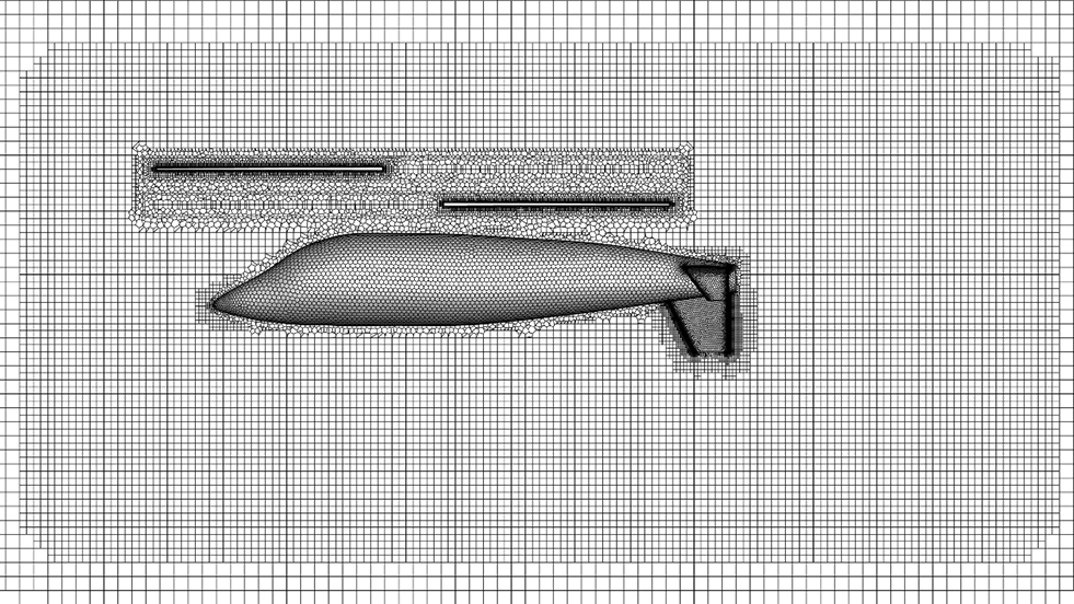
Figure 3: The sliding mesh system

2.5 Simulation Settings

To speed up the convergence and reduce computation time, the steady-state simulation of the flow field is firstly calculated by the moving reference frames method, and then the steady-state results are used as the initial values of transient analysis of the sliding mesh method. The time step of transient analysis is set as the time when the main rotor rotates 1∘ . Each time step contains 20 sub-iterations.

3  Validation

3.1 Caradonna & Tung Rotor

The Caradonna & Tung (CT) rotor with experimental data [27] is utilized to verify the validity of the constructed numerical method. This rotor has two rectangular blades without torsion, and the blades use a NACA0012 profile. The diameter is 2.286 m, and the cord is 0.1905 m. The hover state of 8∘ collective pitch and 0.439 tip Mach number is simulated. Fig. 4 compares the pressure distributions at different spanwise sections between the experiment and this simulation. The pressure distributions of the experiment and this simulation are almost the same, which validates the numerical method constructed in this paper.

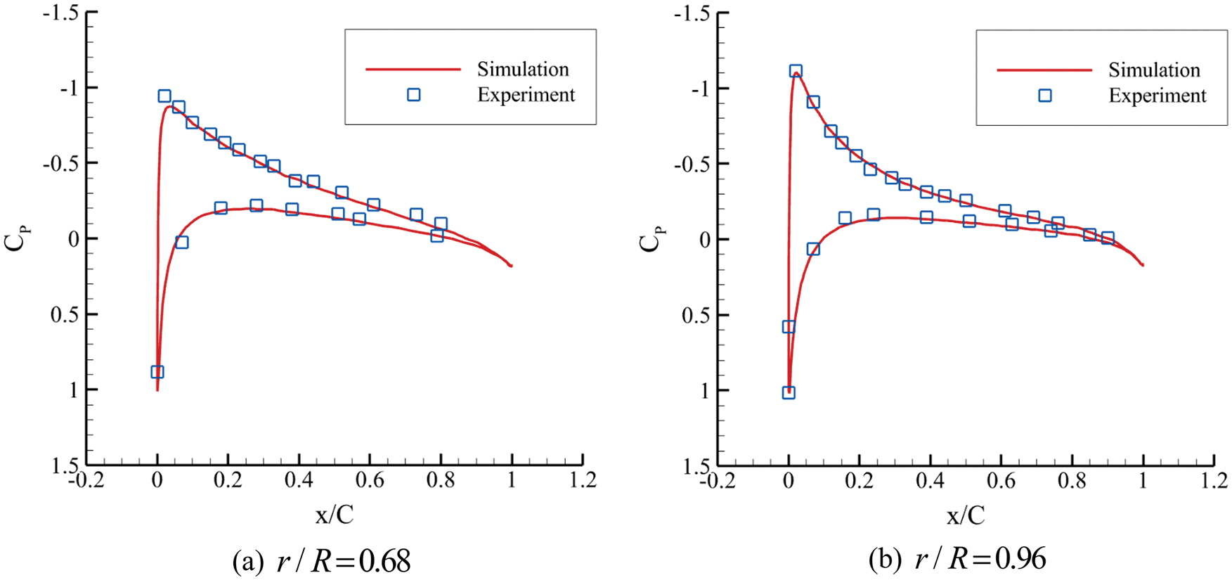
Figure 4: Pressure distributions of blade sections in hover (CT rotor)

3.2 Harrington 2 Rotor

The Harrington 2 rotor is a coaxial rotor from the reference [4], which is widely used to verify the validity of numerical simulations for coaxial rotors. This coaxial rotor has two rectangular blades for each rotor, and the thickness ratio of the blades is tapered. The diameter is 7.62 m, and the cord is 0.4572 m. Then, the cases of 0.293 Mach number and 1∘ differential collective pitch are calculated in this simulation. Fig. 5 presents the results of this simulation and the experiment. Although there is a slight discrepancy for low thrust coefficients, the variations of the calculated thrust coefficient and torque coefficient are consistent with the experiment. Thus, the constructed numerical method can be used for coaxial configurations.

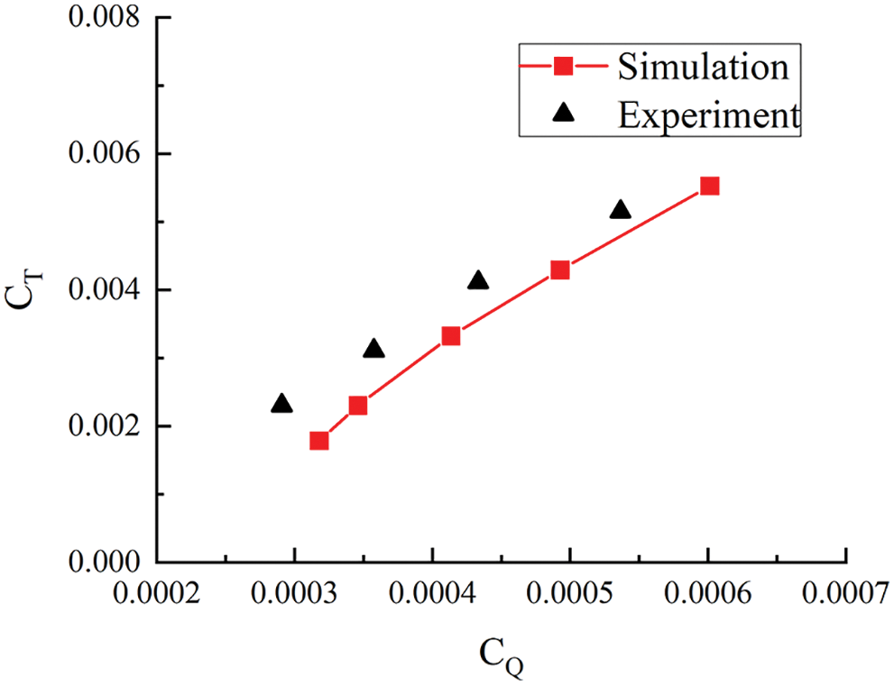
Figure 5: Thrust coefficient and torque coefficient for Harrington 2 rotor

4  Aerodynamic Interactions

In this section, cases of the isolated single rotor, isolated coaxial rotor, and the whole helicopter are calculated, and the aerodynamic interactions between these components are analyzed in hover and forward flights. The simulation conditions are 500 m height, 0.566 Mach number of the blade tip, and 8∘ collective pitch of the main rotors.

4.1 Grid Refinement Study

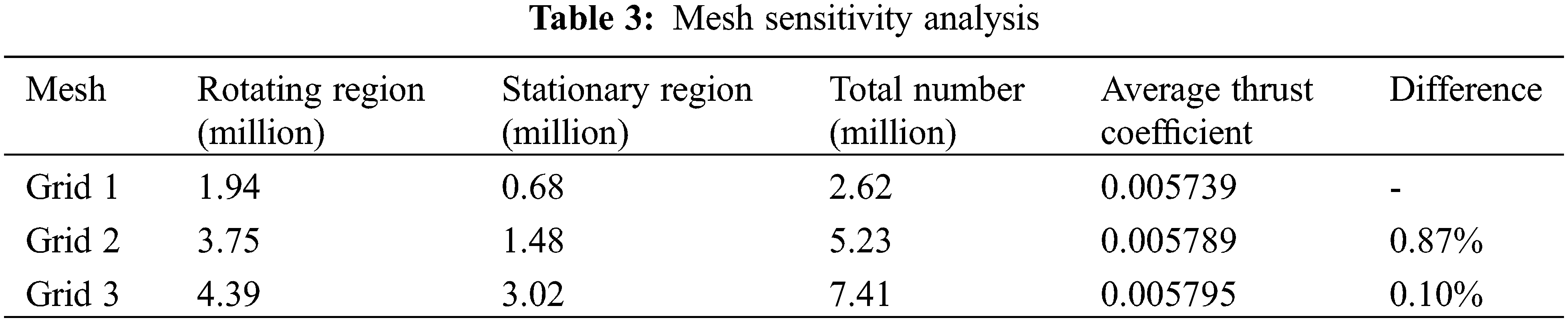
The hover state of the isolated single rotor is calculated with three kinds of grid sizes. Each grid is divided into two regions, the rotating region, and the stationary region. The grids of both regions are refined. The average thrust coefficient ( CT ) in one revolution is used to analyze the mesh sensitivity. The results are shown in Table 3. The difference of CT between Grid 1 and Grid 2 is 0.87%, while the difference of CT between Grid 2 and Grid 3 is 0.1%. Compared with Grid 1 and Grid 2, the improvement of CT between Grid 2 and Grid 3 is much smaller. In view of computational costs, the size distribution of Grid 2 is used in the following simulations.

4.2 Aerodynamic Interactions in Hover

4.2.1 Rotor-Rotor Aerodynamic Interactions

Fig. 6 presents the Z velocity contours of the isolated single rotor and the isolated coaxial rotor in hover. It can be seen that the induced velocity of the isolated coaxial rotor is larger than that of the isolated single rotor. In addition, the induced velocity of the lower rotor is affected by the upper rotor, which reduces the effective angle of attack. Then, the pressure distributions of the blade section changed. Fig. 7 presents the pressure distributions of the upper and lower rotors when the upper and lower blades encounter each other. The negative peak pressure of the lower rotor is smaller than that of the upper rotor, and the discrepancy increases at the outboard of the blade. This demonstrates the velocity distribution above.

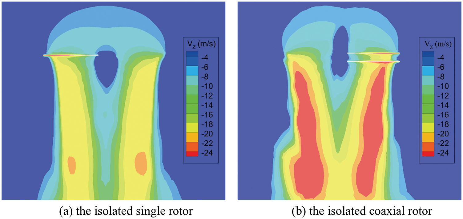
Figure 6: Z velocity contours of the rotors in hover (m/s)

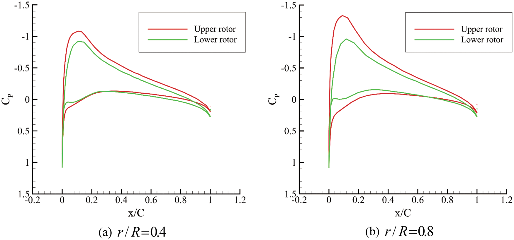
Figure 7: Pressure distributions of blade sections in hover (Coaxial rotor)

Fig. 8 presents the variations of transient thrusts for the isolated single rotor and the isolated coaxial rotor in one revolution. The 0∘ azimuth is defined as the position where one blade of the upper rotor parallels the longitudinal axis of the fuselage. Although the thrust of the isolated single rotor has little change, it appears to have three-per-revolution variation characteristics. This is in accordance with the number of blades. Differently, six periodic variations of thrusts can be seen for the isolated coaxial rotor in one revolution. This is due to the blades of the upper and lower rotors meeting each other at every 60∘ . In one period of 60∘ , the thrust increases firstly. Then, it drops at the azimuth of 30∘ where the upper rotor and lower rotor blades are in the same vertical plane. As described previously, the distance between the upper and lower rotor blades is closest, which results in severe aerodynamic interactions and vibration loads. Furthermore, the average thrust of the upper and the lower rotors is smaller than that of the isolated single rotor. The reason is that the induced velocity of the coaxial rotor reduces the effective angle of attack, which is explained previously.

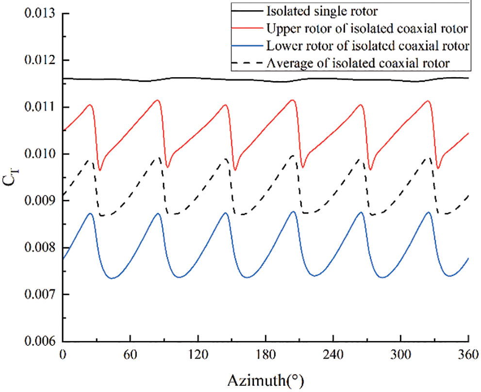
Figure 8: Rotor transient thrusts of the rotors in hover

4.2.2 Rotor-Fuselage Aerodynamic Interactions

Fig. 9 presents the Z velocity distributions of the plane 0.4 m below the lower rotor disc at the azimuth of 0∘ . At this azimuth, both one upper blade and one lower blade are parallel to the longitudinal axis of the fuselage. Compared with the isolated coaxial rotor, the downwash velocity of the coaxial rotor decreases due to the existence of the fuselage.

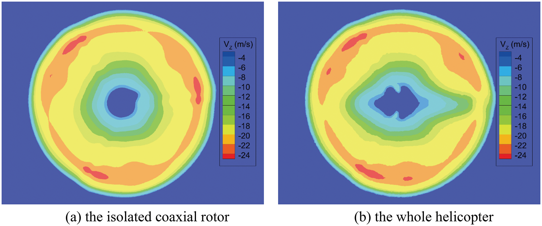
Figure 9: Z velocity distributions below the lower rotor disc (m/s)

Fig. 10 compares the transient thrusts between the isolated coaxial rotor and the coaxial rotor in the whole helicopter. The thrusts of the upper and lower rotors in the whole helicopter are larger than that of the isolated coaxial rotor. This indicates that the existence of the fuselage has a positive effect on the rotor lift capability.

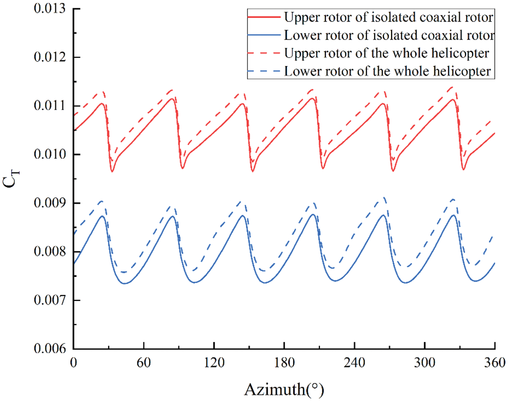
Figure 10: Rotor thrusts for the isolated coaxial rotor and the coaxial rotor in the whole helicopter

4.3 Aerodynamic Interactions in Forward Flight

4.3.1 Rotor-Rotor Aerodynamic Interactions

The cases of the isolated single rotor, the isolated coaxial rotor, and the whole helicopter are calculated at advance ratios of 0.1, 0.2, and 0.3.

Fig. 11 presents the transient thrusts of the rotors at these advance ratios. It can be seen that the thrust of the coaxial rotor is still smaller than that of the single rotor due to the interactions between the coaxial rotors. Moreover, the periodic thrust variation of the isolated single rotor remains three-per-revolution. However, the addition of the forward speed changes the periodic thrust variation of the coaxial rotors. Compared with the hover state, the periodic thrust variation of the upper and lower rotors changes to three-per-revolution in forward flight. Furthermore, the thrust of the upper rotor oscillates at the azimuths of 30∘ , where the upper rotor’s and lower rotor’s blades meet each other. This oscillation interrupts the increasement of the thrust, which makes the variation trend different from the single rotor. This phenomenon of thrust oscillation also emerges at the azimuth of 90∘ for the lower rotor. Differently, this oscillation is slight. With the increasement of the advance ratio, the thrusts of the rotors increase, and the oscillation becomes more obvious.

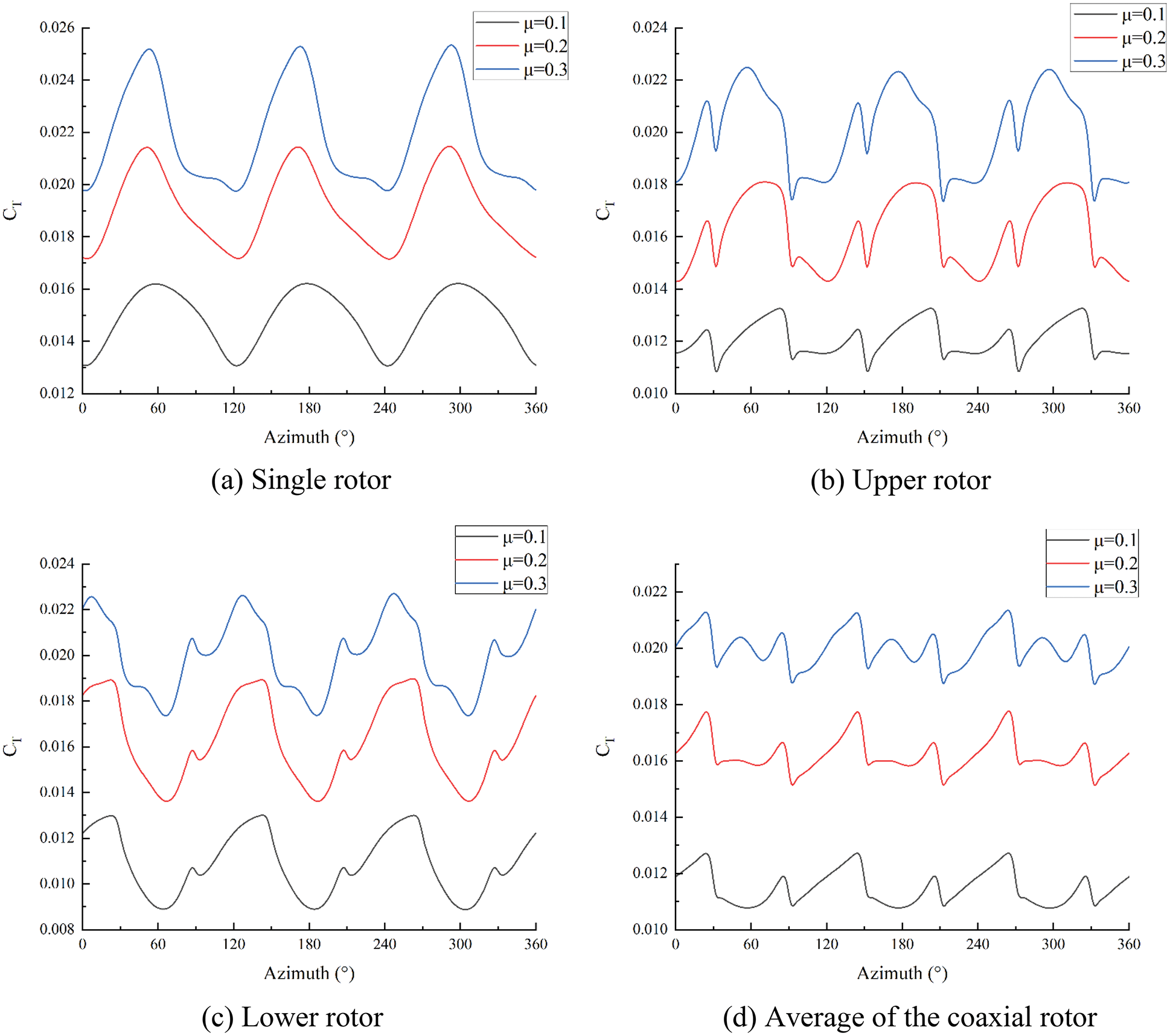
Figure 11: Rotor thrusts at different advance ratios

To identify the interactions of the coaxial rotors in forward flights, the pressure distributions of the isolated single rotor and coaxial rotors at the advancing and retreating sides are compared, as shown in Fig. 12. The disc azimuth here is 90∘ where one upper blade is on the advancing side and one lower blade is on the retreating side. The upper and lower rotors also meet at this disc azimuth. At the advance ratio of 0.1, the pressures of the upper and lower blades are smaller than that of the isolated single rotor. The discrepancy between the lower rotor and the single rotor is larger than that between the upper rotor and the single rotor. This indicates that the main interaction of the coaxial rotor in forward flight originates from the influence of the upper rotor on the lower rotor. With the increment of the advance ratio, the interaction of the coaxial rotor weakens. In particular, the pressure distributions of the upper rotor and the single rotor are almost the same at the advance ratio of 0.3. Nevertheless, the upper rotor still impacts the lower rotor at higher advance ratios. This influence results in a pressure increase in the lower surface for the lower rotor.

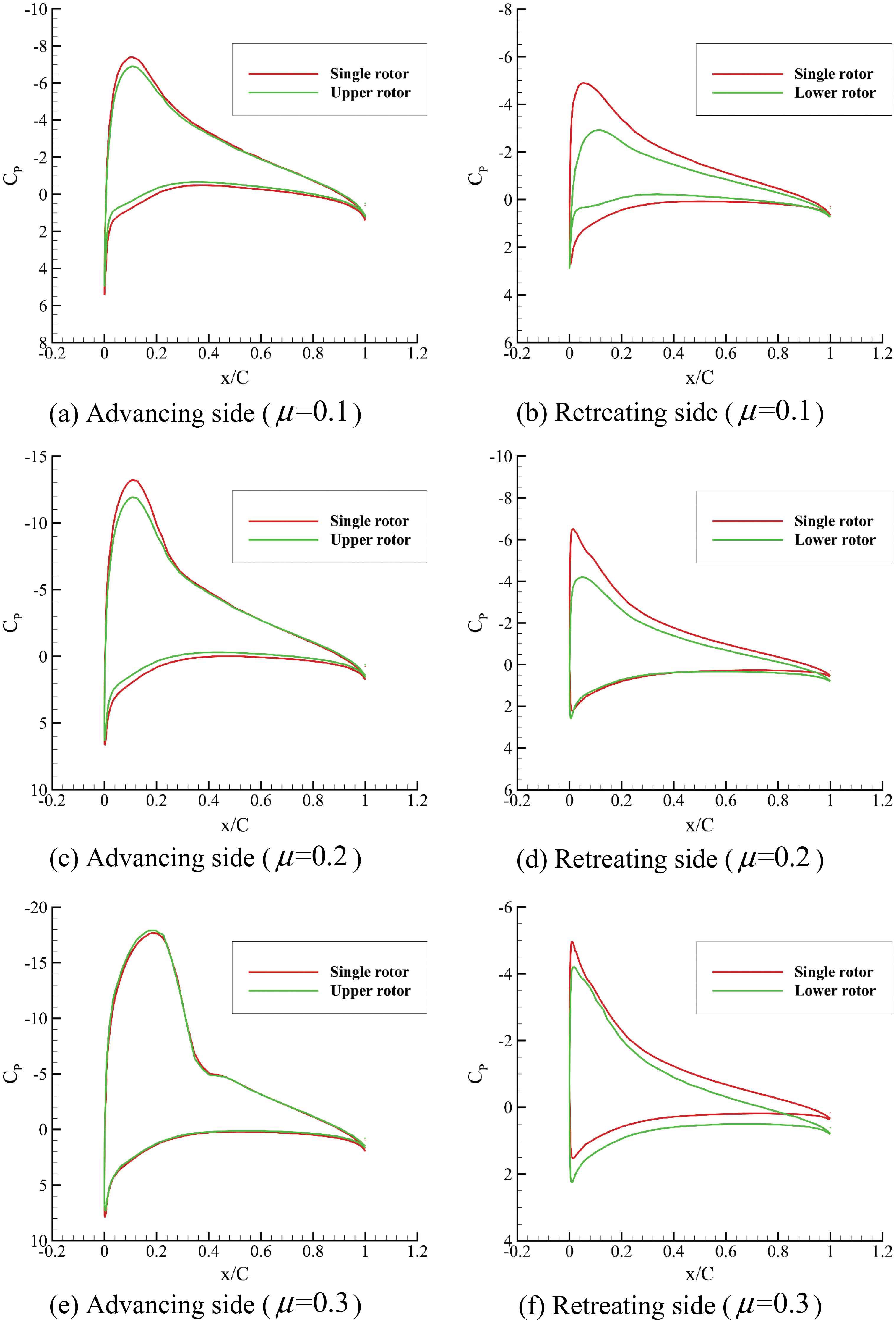
Figure 12: Blade section pressure distributions of advancing and retreating sides ( r/R=0.8 )

4.3.2 Rotor-Fuselage Aerodynamic Interactions

Fig. 13 presents the velocity contours in the longitudinal cross-section at different advance ratios. At the advance ratio of 0.1, the wake of the main rotors is blocked by the fuselage on a large scale, which causes severe aerodynamic interactions. As the advance ratio increases, the wake of the main rotor tilts in the backward direction. The impact of the main rotor downwash on the fuselage is weakened at the advance ratio of 0.2. Moreover, the downwash of the main rotor has little influence on the fuselage at the advance ratio of 0.3. This phenomenon is consistent with the variation of fuselage lift, as shown in Fig. 14. The fuselage lift coefficient is negative because of the rotor downwash. However, the value of the fuselage lift coefficient decreases with the increment of the advance ratio. These indicate that the interactions between the main rotor and the fuselage decay with the increase of the advance ratio.

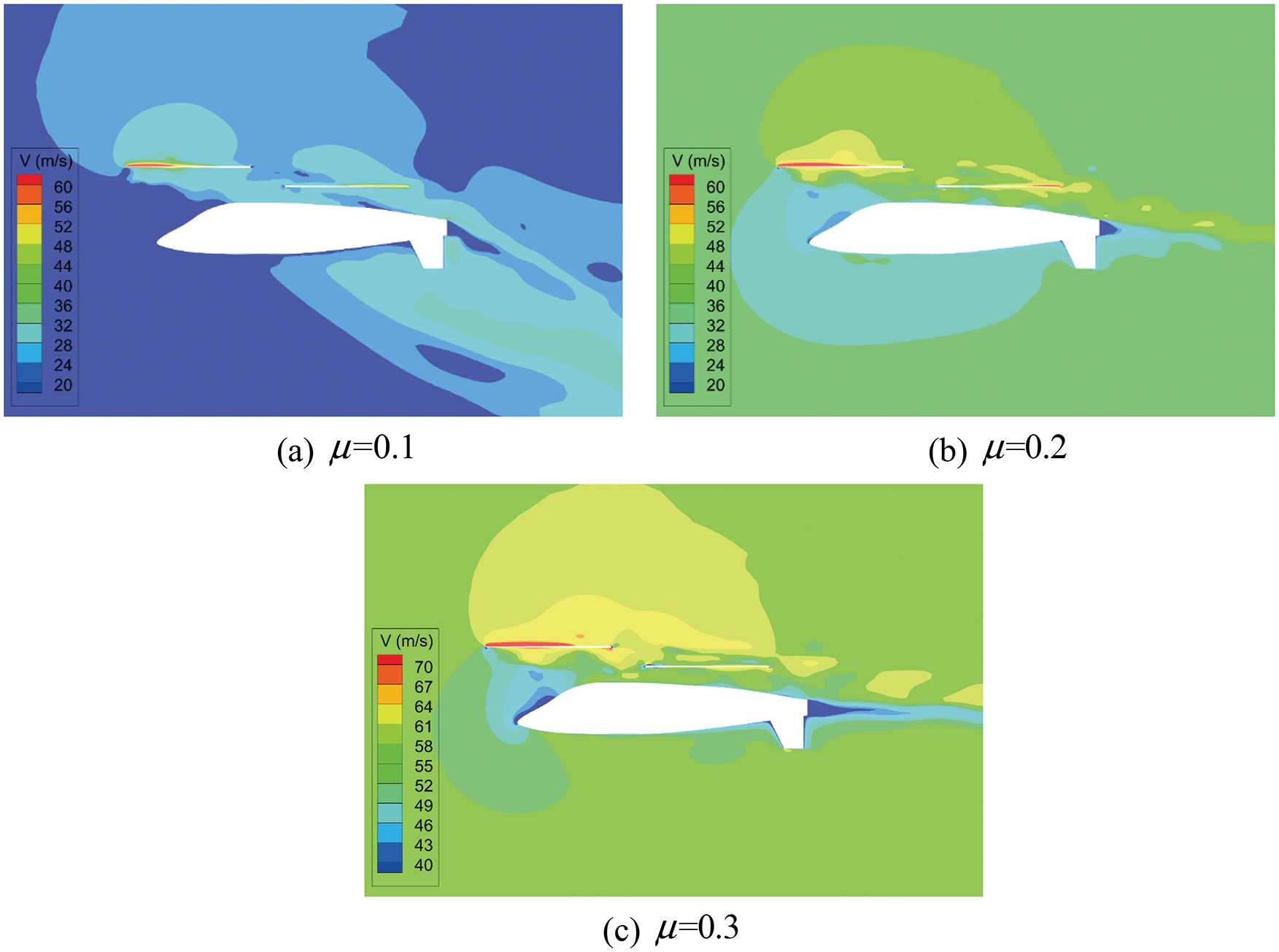
Figure 13: Velocity contours of the whole helicopter in forward flights

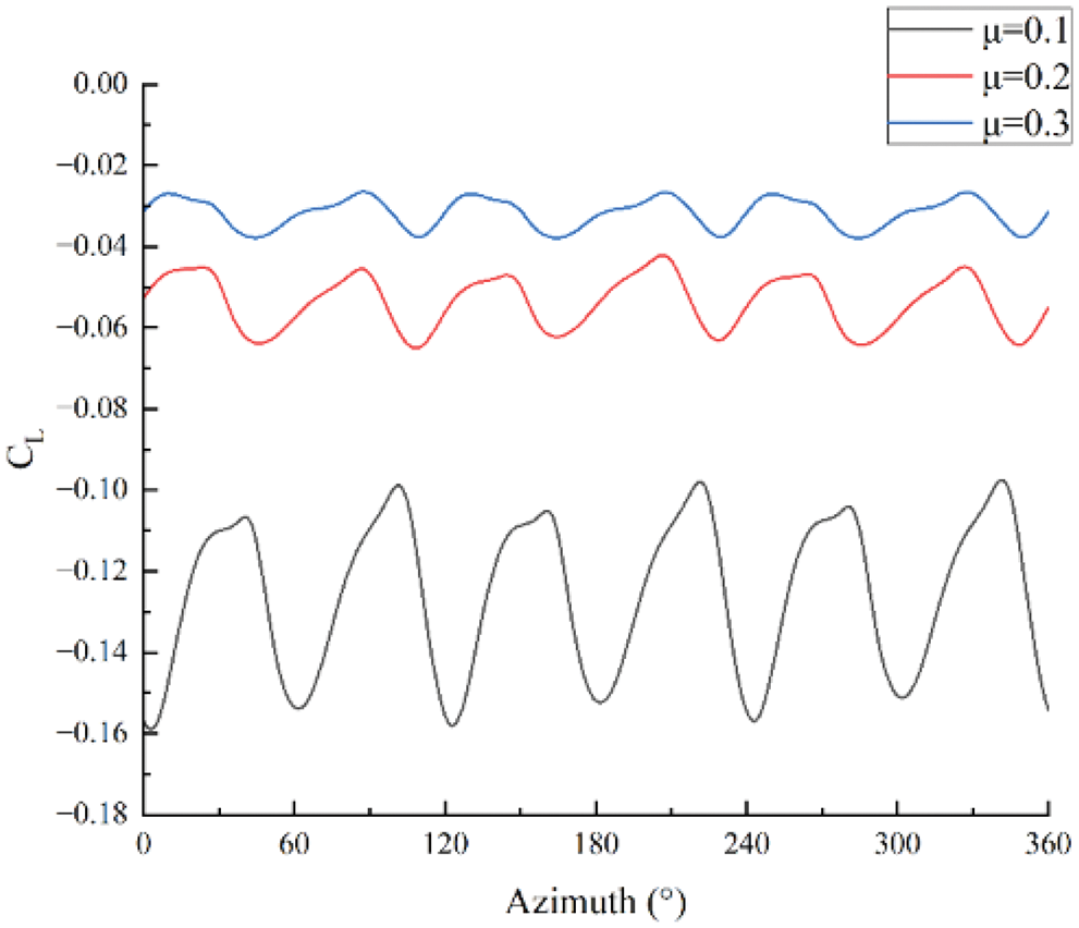
Figure 14: Lift coefficients of the fuselage at different advance ratios

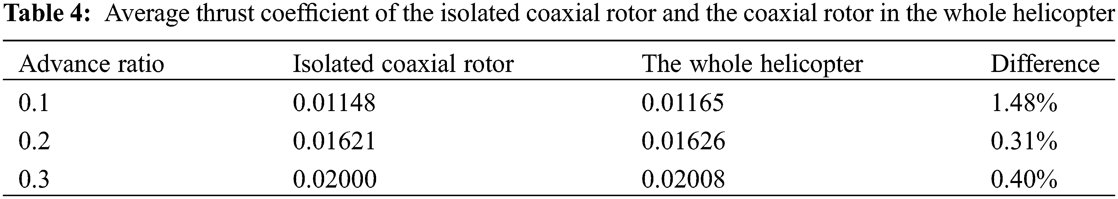
Table 4 illustrates the fuselage’s effect on the coaxial rotor’s average thrusts in one revolution. Because the downwash of the main rotor is blocked by the fuselage, the average thrust of the main rotor increases. However, this effect is weakened when the advance ratio increases, which is in accordance with Fig. 13.

5  Conclusion

Based on the sliding mesh method, a numerical method for coaxial rotor helicopter aerodynamic interaction simulation is constructed. The rotor-rotor interactions and rotor-fuselage interactions are analyzed in hover and forward flights. The following conclusions are obtained:

1.    Compared with the isolated single rotor, the aerodynamic interaction of the two rigid coaxial rotors significantly influences the induced velocity and pressure distribution in hover. This interaction also reduces the thrust of the isolated coaxial rotor.

2.    Compared with the hover state, the periodic thrust variation of the upper rotor and lower rotor changes from six-per-revolution to three-per-revolution in forward flights. The encounter of the upper and lower rotors results in the oscillation of the transient thrusts.

3.    The thrust of the coaxial rotor increases due to the fuselage’s blocked downwash of the coaxial rotor. This indicated that the fuselage positively affects the lift capability of the coaxial rotor.

4.    The interactions between the components of the coaxial helicopter decay with the advance ratio increasing.

Funding Statement: This work was supported by Rotor Aerodynamics Key Laboratory [Grant No. RAL202102-4].

Conflicts of Interest: The authors declare that they have no conflicts of interest to report regarding the present study.

References

1. Cheney, M. C. (1969). The ABC helicopter. VTOL Research, Design, and Operations Meeting, Geogia. [Google Scholar]
2. Ruddell, A. J. (1981). Advancing blade concept (ABC) development test program. 1st Flight Test ConferenceNevada. [Google Scholar]
3. Ruddell, A. J. (1981). Advancing blade concept (ABC) technology demonstrator. NASA-ADA-100181. [Google Scholar]
4. Harrington, D. (1951). Full-scale-tunnel investigation of the static-thrust performance of a coaxial helicopter rotor. NACA-TN-2318. [Google Scholar]
5. Landgrebe, A. J., Bellinger, E. D. (1974). Experimental investigation of model variable-geometry and ogee tip rotors. NASA-CR-2275. [Google Scholar]
6. Ramasamy, M. (2013). Measurements comparing hover performance of single, coaxial, tandem, and tilt-rotor configurations. AHS 69th Annual Forum, Phoenix, AZ. [Google Scholar]
7. Konus, M. F. (2017). Vortex wake of coaxial rotors in hover (Ph.D. Thesis). Mechanical Engineering, University of California, Berkeley, USA. [Google Scholar]
8. Silwal, L., Raghav, V. (2020). Preliminary study of the near wake vortex interactions of a coaxial rotor in hover. AIAA Scitech 2020 Forum. [Google Scholar]
9. Lyu, W., Xu, G. (2018). Interactional effect of propulsive propeller location on counter-rotating coaxial main rotor. Journal of Aircraft, 55(6), 2538–2545. DOI 10.2514/1.C033316. [Google Scholar] [CrossRef]
10. Syal, M., Leishman, J. G. (2012). Aerodynamic optimization study of a coaxial rotor in hovering flight. Journal of the American Helicopter Society, 57(4), 1–15. DOI 10.4050/JAHS.57.042003. [Google Scholar] [CrossRef]
11. Kim, H. W., Brown, R. E. (2010). A rational approach to comparing the performance of coaxial and conventional rotors. Journal of the American Helicopter Society, 55(1), 012003. DOI 10.4050/JAHS.55.012003. [Google Scholar] [CrossRef]
12. Tan, J., Sun, Y., Barakos, G. N. (2018). Unsteady loads for coaxial rotors in forward flight computed using a vortex particle method. The Aeronautical Journal, 122(1251), 693–714. DOI 10.1017/aer.2018.8. [Google Scholar] [CrossRef]
13. Lakshminarayan, V. K., Baeder, J. D. (2010). Computational investigation of microscale coaxial-rotor aerodynamics in hover. Journal of Aircraft, 47(3), 940–955. DOI 10.2514/1.46530. [Google Scholar] [CrossRef]
14. Xu, H., Ye, Z. (2010). Coaxial rotor helicopter in hover based on unstructured dynamic overset grids. Journal of Aircraft, 47(5), 1820–1824. DOI 10.2514/1.C031079. [Google Scholar] [CrossRef]
15. Xu, H., Ye, Z. (2011). Numerical simulation of unsteady flow around forward flight helicopter with coaxial rotors. Chinese Journal of Aeronautics, 24(1), 1–7. DOI 10.1016/S1000-9361(11)60001-0. [Google Scholar] [CrossRef]
16. Zhao, X., Zhou, P., Yan, X., Lin, Y. (2017). Numerical study of aerodynamic performance and flow interaction for coaxial rigid rotor in hover and forward flight. 35th AIAA Applied Aerodynamics ConferenceColorado. [Google Scholar]
17. Deng, J. H., Fan, F., Liu, P. A., Huang, S. L., Lin, Y. F. (2019). Aerodynamic characteristics of rigid coaxial rotor by wind tunnel test and numerical calculation. Chinese Journal of Aeronautics, 32(3), 568–576. DOI 10.1016/j.cja.2018.12.026. [Google Scholar] [CrossRef]
18. Park, S. H., Kwon, O. J. (2020). Numerical study about aerodynamic interaction for coaxial rotor blades. International Journal of Aeronautical and Space Sciences, 22(2), 277–286. DOI 10.1007/s42405-020-00310-6. [Google Scholar] [CrossRef]
19. Jia, Z., Lee, S. (2021). Aerodynamically induced noise of a lift-offset coaxial rotor with pitch attitude in high-speed forward flight. Journal of Sound and Vibration, 491, 1–34. DOI 10.1016/j.jsv.2020.115737. [Google Scholar] [CrossRef]
20. Versteeg, H. K., Malalasekera, W. (2007). An introduction to computational fluid dynamics: The finite volume method. England: Pearson Education. [Google Scholar]
21. Hinze, J. O. (1975). Turbulence. New York: McGraw-Hill. [Google Scholar]
22. Patankar, S. V. (1980). Numerical heat transfer and fluid flow. New York: Hemisphere Publishing Corporation. [Google Scholar]
23. Menter, F. R. (1994). Two-equation eddy-viscosity turbulence models for engineering applications. AIAA Journal, 32(8), 1598–1605. DOI 10.2514/3.12149. [Google Scholar] [CrossRef]
24. Mathur, S. (1994). Unsteady flow simulations using unstructured sliding meshes. Fluid Dynamics Conference, Colorado Springs, CO. [Google Scholar]
25. Walsh, D., Weiner, S., Arifian, K., Bagai, A., Lawrence, T. et al. (2009). Development testing of the sikorsky X2 technologyTM demonstrator. The 65th Annual Forum of the American Helicopter Society InternationalGrapevine, TX. [Google Scholar]
26. Kim, H. W., Kenyon, A. R., Duraisamy, K., Brown, R. E. (2008). Interactional aerodynamics and acoustics of hingeless coaxial helicopter with an auxiliary propeller in forward flight. 9th International Powered Lift ConferenceLondon. [Google Scholar]
27. Caradonna, F. X., Tung, C. (1981). Experimental and analytical studies of a model helicopter rotor in hover. NASA-TM-81232. [Google Scholar]
Cite This Article
Copyright © 2023 The Author(s). Published by Tech Science Press.
This work is licensed under a Creative Commons Attribution 4.0 International License , which permits unrestricted use, distribution, and reproduction in any medium, provided the original work is properly cited.
Downloads
Citation Tools