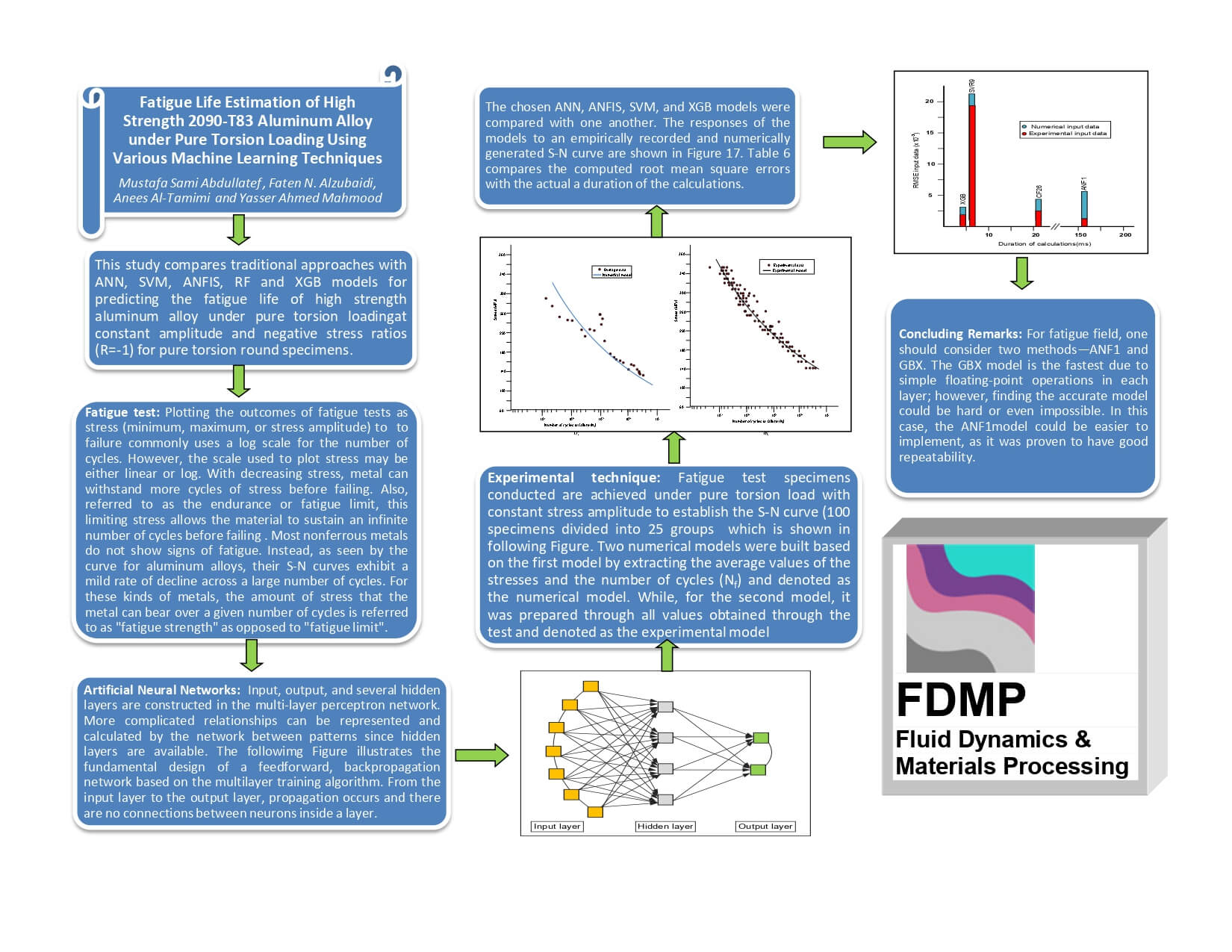
Fatigue Life Estimation of High Strength 2090-T83 Aluminum Alloy under Pure Torsion Loading Using Various Machine Learning Techniques

Nomenclature

1  Introduction

Fatigue life is the most important issue that influences the structure and material engineering leading to an effect on the life of the human. The fatigue damage is the primary cause of failure situations which has been the area of the research during the past few years, where they have been demonstrated that the root cause of 80% of incidents involving applied structures. The fatigue phenomena has been extensively studied using machine learning techniques when one or more of the following conditions exist; Firstly, there is a significant amount of data accessible. Secondly, a precise solution using physics-based mathematical techniques is not feasible; and finally, if the data range is complex or erratic, the machine learning models are appropriate [1].

The most popular kinds of fatigue testing are S-N tests, often known as Wöhler tests. These tests are simulated to component the fatigue life and offer engineers useful data for the design process. It is constructed by using empirical formulas based on experimental data due to the nonlinearity and several other factors that affect on it. Several empirical formulas, including the Dengel representation with two parameters a and b, the Basquin equation with a logarithmic scale and two parameters a and b, are used to find S-N curves. We can enhance the quality of the data correction by using the inflection point method developed by Palmgren and Stromeyer with two parameters. The Corson equation, which has three parameters (A, E, and d), and the Weibull equation, which has four parameters, are both significantly inaccurate and inconsistent [2]. Since achieving the fatigue S-N curve has been extremely challenging; therefore it is an imperative objective for the designer to obtain the curve fully and consistently. One of the artificial intelligence techniques that have been used successfully in a variety of engineering applications is artificial neural networks. Although multivariable nonlinear mathematical modelling accuracy is extremely challenging to achieve using conventional analytical techniques, it can be correctly represented by ANN due to its massively parallel structure. Many researchers utilize ANNs to forecast the fatigue life of materials because they are excellent at characterizing fatigue processes [3].

For instance, artificial neural networks were used by Dharmadhikari et al. [4], who examined the potential of each deep neural network (DNN) structure to identify fatigue cracks during two separate phases of fatigue failure. With two-phase accuracy rates of 94.26 percent and 98.94 percent for the feature-free network, it was found that it perform better than the feature-based network; this implies that feature-free DNNs can replicate features more accurately, even if they are black boxes by design, and can make it easier to choose between signal processing methods that have the similar problems. In the study by Mohanty et al. [5], ANN was used to predict the fatigue fracture propagation life of the aluminum alloys 7020-T7 and 2024-T3 under the influence of the load ratio. In this study, numerous phenomenological models have been put forward for forecasting the fatigue life of the components under the influence of the load ratio to calculate the impact of the mean load. Moreover, using an artificial neural network (ANN) develop an autonomous prediction methodology to evaluate the constant amplitude loading fatigue life. Himmiche et al. [6] illustrated the two different ANN techniques (Radial basis function network (RBFN) and extreme learning machine (ELM)) that could be used to predict the minor crack formation due to fatigue. These two techniques have ability to create and anticipate the emergence of microscopic fatigue cracks in different materials, where the variety of stress levels and ratios (R) are considered in the works.

Bentéjac et al. [7] introduced a novel approach that examines the XGBoost technology. In this work, a scalable assembly method based on scaling improvement has been established as a dependable and potent remedy for machine learning problems. This study offers a useful analysis of the training efficiency, generalization effectiveness, and parameter. Additionally, a comparison of XGBoost with gradient boosting, random forests, and default settings were concluded in addition to using the properly tailored models. Basak et al. [8] studied the generalization error linked to obtaining overall performance with the role of Support Vector Regression (SVR) technology. The SVR technology has been used in a variety of applications, including time series, risky and noisy financial forecasting, convex quadratic programming, loss function alternatives, and approximation of difficult geometrical analyses.

Branco et al. [9] investigated the potential use of the cumulative strain energy density as a parameter to measure fatigue in high-tech, strain-controlled steels. First, nine steel types were chosen from three multiphase families, representing a range of elemental compositions and heat treatment techniques, and their cyclic stress-strain responses were examined. Then, the suggested model’s predictive abilities were contrasted with those of alternative strain- and energy-based methods. They discovered that when the strain amplitude increases, the cumulative strain energy density falls. Additionally, it was discovered that a power function may be used to connect the cumulative strain energy density and fatigue life. Macek et al. [10] added to the understanding of fracture mechanisms for fatigue performance by examining the fracture surface topography of X8CrNiS18-9 austenitic stainless steel specimens under various loading conditions and notch radii. Cases with three distinct notch radius and stress amplitude values were analyzed, and using an optical confocal measurement device, the areas covering the whole surface of the fracture topographies were calculated.

Abdullatef et al. [11] used traditional analytical techniques to predict fatigue life (number of cycles to failure) for composite materials that are constructed by stacking four layers of fibreglass-reinforced polyester resin. These plies were tested in completely reversible tension-compression under dynamic load (fatigue test) at stress ratio  R=−1 . A trustworthy and accurate method for estimating fatigue life is the ANN. The networks employed are the Radial Bases Function Neural Network (RBFNN), the Generalized Regression Neural Network (GRNN), and the Feed Forward Neural Network (FFNN). Through a comparison of the experimental outcomes, it was determined that ANN techniques are superior to traditional methods for prediction. The findings demonstrate the effectiveness of RBFNN as a tool for predicting and optimizing the fatigue life of fibreglass-reinforced composites. Stress load and angle of orientation are inputs to the network, and the network output is the number of cycles until failure.

This study compares traditional approaches with ANN, SVM, ANFIS, RF and XGB models for predicting the fatigue life of high strength aluminum alloy 2090-T83 under pure torsion loadingat constant amplitude and negative stress ratios ( R=−1 ) for pure torsion round specimens.

2  Fatigue Test

Plotting the outcomes of fatigue tests as stress (minimum, maximum, or stress amplitude) to Nf to failure commonly uses a log scale for the number of cycles. However, the scale used to plot stress may be either linear or log. With decreasing stress, metal can withstand more cycles of stress before failing. Also, referred to as the endurance or fatigue limit, this limiting stress allows the material to sustain an infinite number of cycles before failing [12]. The maximum stress that a metal can withstand for an infinitely high number of cycles with a 50% failure chance is known as the fatigue (endurance) limit, or Sf , and it is represented by the S−N curve’s horizontal region. Most nonferrous metals do not show signs of fatigue. Instead, as seen by the curve for aluminum alloys, their S-N curves exhibit a mild rate of decline across a large number of cycles. For these kinds of metals, the amount of stress that the metal can bear over a given number of cycles is referred to as “fatigue strength” as opposed to “fatigue limit”. Each table of fatigue strengths must state the number of cycles for which the strengths are displayed because there is no set number of cycles. Falsely referred to as the fatigue limit, the fatigue strength of nonferrous metals is usually at 108 or 5∗108 stress cycles [13].

3  Artificial Neural Networks

The multi-layer perceptron, a type of neural network trained using the backpropagation method (backpropagation neural network), is the most effective in applications for engineering fields. Thus, this approaches is used the back-propagation neural network. It gets its name from the fact that the back-propagation network learns by reflecting errors backward from input neurons to output neurons. In Fig. 1, a single artificial neuron’s structure is presented. The following formula is used to calculate the weighted sum of the input components:

Sj=∑i=1nwijxi−θj (1)

where  xi is the output of the ith neuron in the previous layer,  wij is the weight between the ith neuron and the jth neuron in the next layer; the intrinsic threshold, or θj , can be thought of as a single weight with a negative sign; and Sj is the weighted sum of a jth neuron for input received from the preceding layer with n neurons. The output of the jth neuron yj is calculated using the sigmoid function once the weighted sum Sj has been computed:

yj =f(Sj)=11+exp(−ηSj) (2)

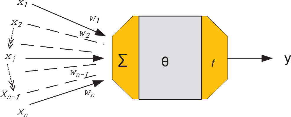
Figure 1: An artificial neuron’s schematic structure with input units

The semi-linear region’s slope is managed by the constant  η . Except for the input layer, all layers exhibit sigmoid nonlinearity [14].

Input, output, and several hidden layers are constructed in the multi-layer perceptron network. More complicated relationships can be represented and calculated by the network between patterns since hidden layers are available. Numerous researchers have shown that the three-layers and multi-layer perceptron can complete classification tasks of any difficulty, depending on how many neurons are present in the hidden layer, with complexity. Depending on many factors, such as the number of neurons in each layer may change. Fig. 2 illustrates the fundamental design of a feedforward, backpropagation network based on the multilayer training algorithm. From the input layer to the output layer, propagation occurs and there are no connections between neurons inside a layer. To reduce the discrepancy between the actual and desired outputs, the network is given an assortment of input and output sequences that are matching and the connection strengths or weights of the interconnections are automatically altered. This method of neural network training is known as supervised learning. The cost function is the mean square difference between the desired and actual network outputs, and it is minimized using a gradient search technique. A significant number of training sets and cycles are used for the network’s training (epochs). The root means square error is obtained by adding the squares of the errors for each neuron in the output layer, dividing by the total number of neurons in the output layer to obtain an average, and taking the square root of that average. The root mean square error produces the convergence criteria is represented mathematically as [15]:

εRMS=∑i=1m⁡(di−yi)2m (3)

where  m is the number of neurons in the output layer, yi and di represent the actual output and desired values for the ith output neuron, respectively.

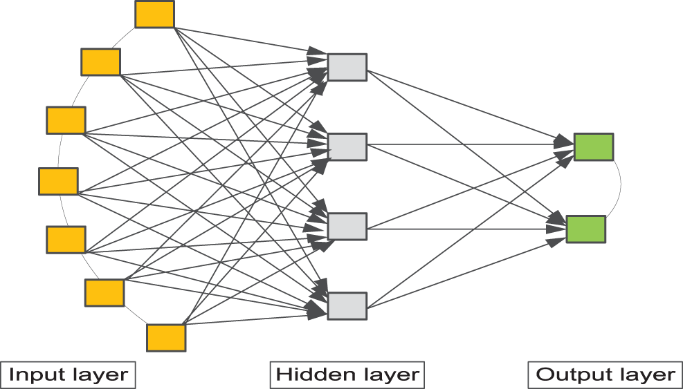
Figure 2: Basic elements of a multi-layer perceptron-based feed-forward, back-propagation network

4  Adaptive Neuro-Fuzzy Inference System

The Sugeno type of fuzzy model is used by ANFIS, a neuro-fuzzy system, to avoid employing defuzzification. It provides the rules’ formulae. The fuzzy inference system in this system comprises two inputs, m1 and m2 , and one output, k. The following statements provide a common rule set for the Sugeno model with two fuzzy if-then rules:

Rule 1 : If m1 is X1 and m2 is Y1;  then f1=x1m1+y1m2+z1 .

Rule 2 : If m1is X2 and m2 is Y2;  then f2=x2m1+y2m2+z2 .

The coefficients of the first-order linear polynomial linear functions are; xi , yi , and (zi = 1, 2), while X1 , Y1 , X2 , and Y2 are fuzzy sets. As shown in Fig. 3, ANFIS has five-layer architecture. Input, fuzzification, rule, normalization, and output layers are included. The fuzzification layer produces the inputs’ fuzzy numbers, also, the others fuzzy numbers that can be used which are including the triangle, trapezoid, and Gaussian fuzzy numbers. Eq. (4) is frequently used with a triangular fuzzy number.

f(x; a, b, c)={0,              x≤ax−ab−a,       a≤x≤bc−xc−b,       b≤x≤c0,               c≤x (4)

where a and c are the triangular bases, and b is the top. Rules are developed following the fuzzification of the inputs. By using these guidelines, normalization is created. An output layer provides the system’s outcomes in the end [16].

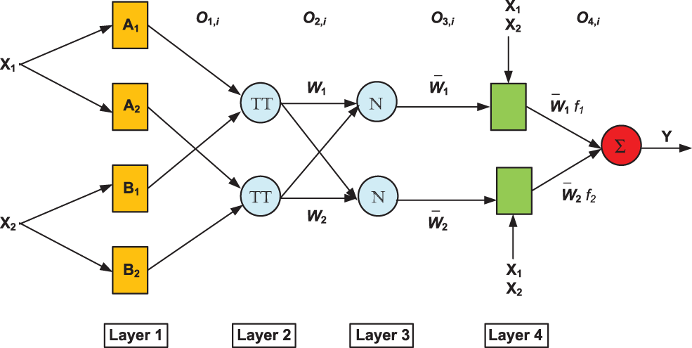
Figure 3: ANFIS structure [16]

5  Experimental Technique

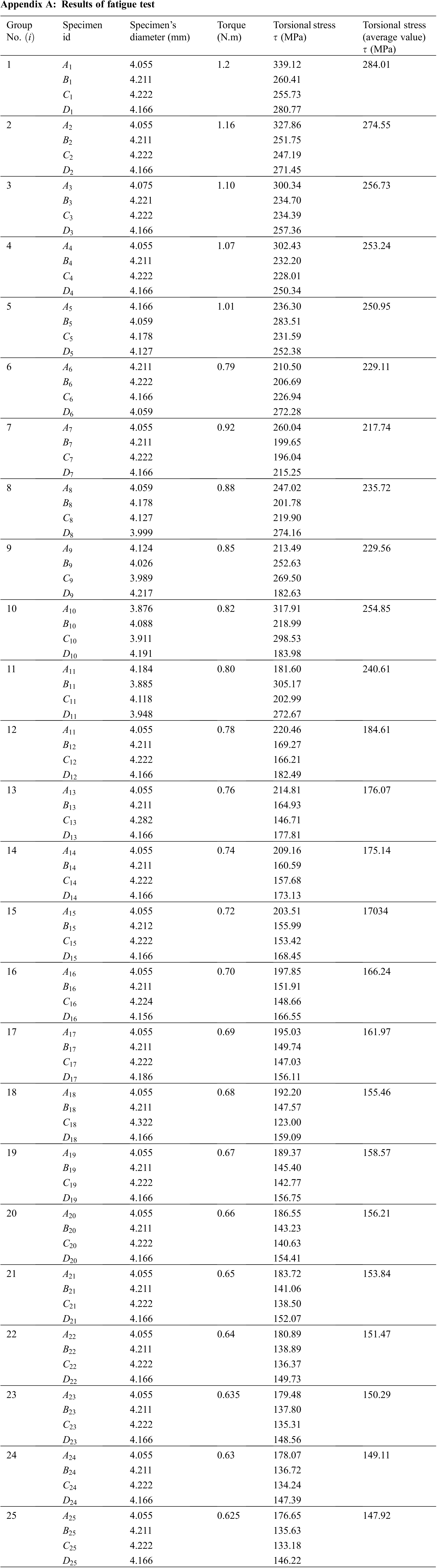
This research was carried out on high-strength aluminum alloy 2090-T83. Developed for high-strength aerospace applications, it is an aluminum-lithium alloy. When compared to other aircraft alloys, Li-Cu-Al alloy provides 8% reduction in density and 10% higher for the modulus of the elasticity. In addition to the low-density feature, this has unique weight-saving benefits. Alloy 2090-T83 has comparable strengths to other high strength aluminum alloys and higher corrosion resistance [17]. The chemical compositions and the mechanical properties are shown in Tables 1 and 2, respectively. With an average radius of 3.95 mm, the pure torsion round specimens were used for the fatigue tests. The main measurements of the test specimens are shown in Fig. 4. The experiment is conducted by using the fatigue testing machine (AVERY’S 7305) [18], see Fig. 5. With an average radius of 3.95 mm, the pure torsion round specimens were used for these tests. At R=−1 , a constant load amplitude test was conducted while the fatigue test was in place. For each torque level, the four specimens, Ai , Bi , Ci and Di , are used to calculate the fatigue life by plotting the S−N curves. Table 3 presents the results of the average input data which were computed based on the fatigue test results and are displayed in Appendix A.

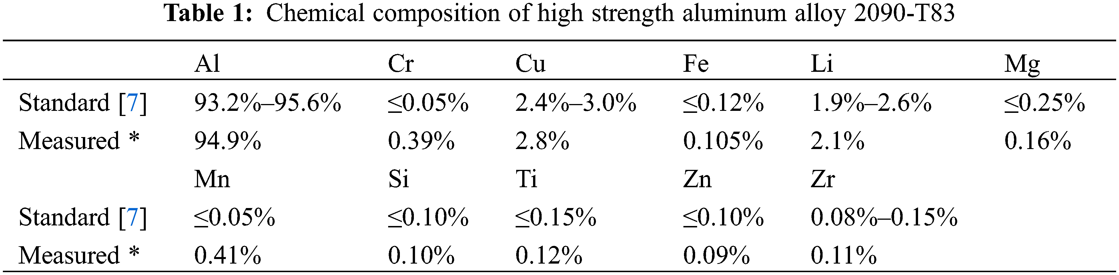
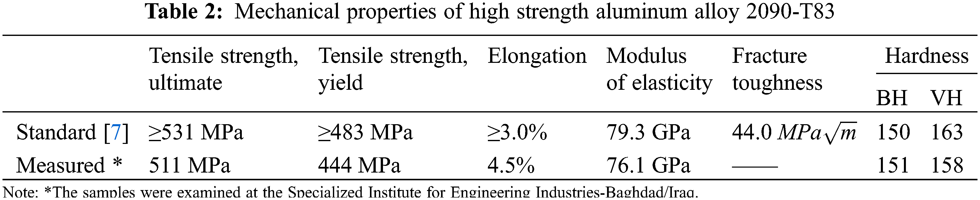
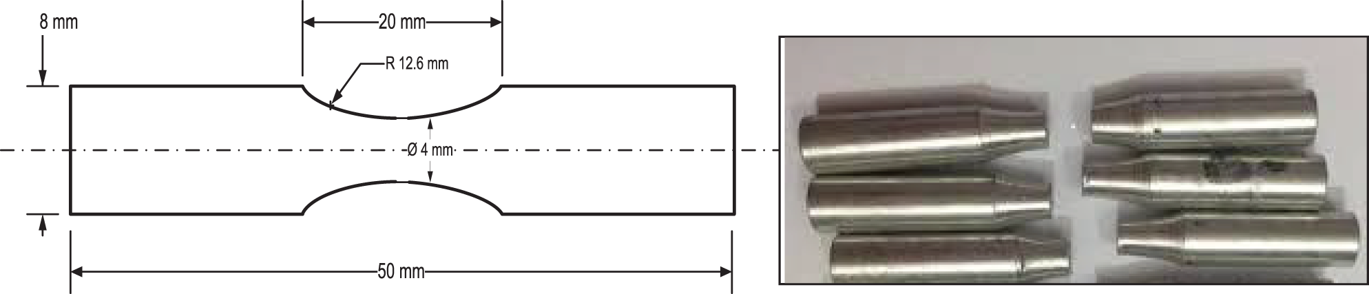
Figure 4: Round specimen fatigue test for pure torsion

Figure 5: AVERY’s 7305 fatigue testing machine

6  Results and Discussion

6.1 Fatigue Test Results

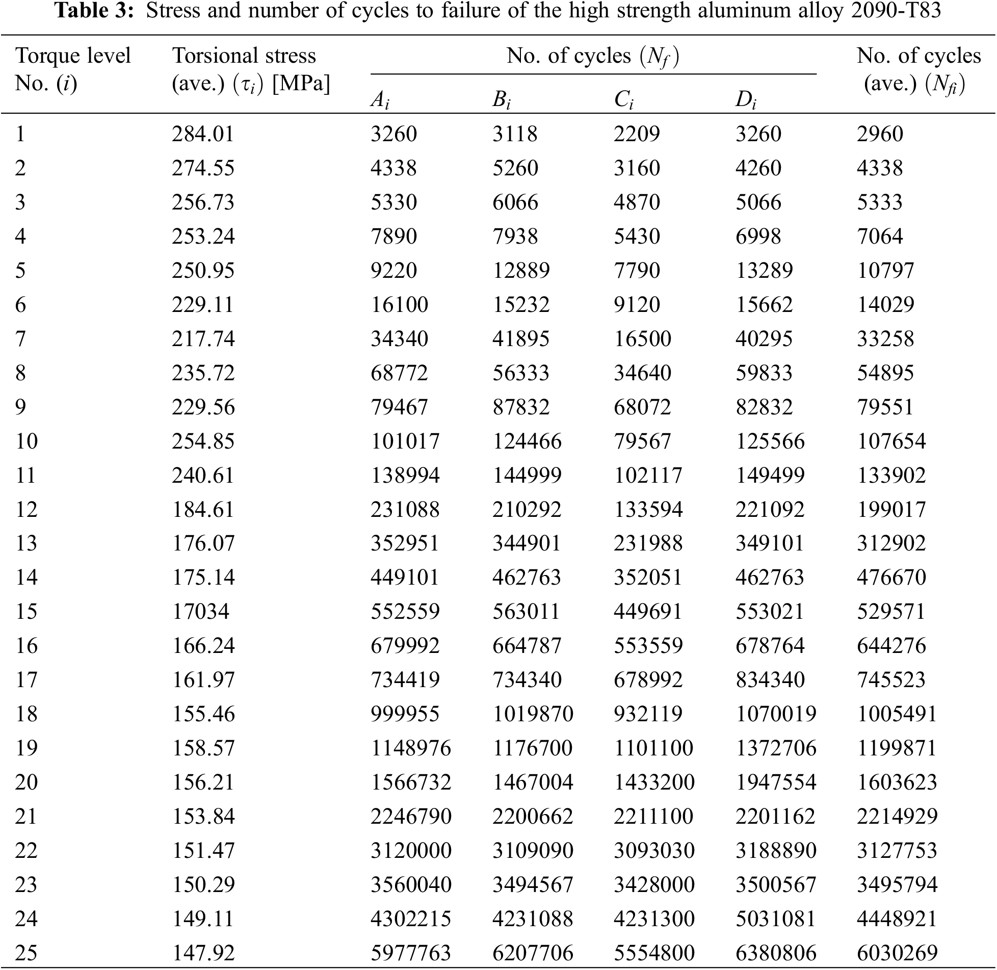
Fatigue test specimens conducted are achieved under pure torsion load with constant stress amplitude to establish the S-N curve (100 specimens divided into 25 groups are listed in Table 3), which is shown in Fig. 6. Two numerical models were built based on the first model by extracting the average values of the stresses and the number of cycles ( Nf ) shown in Eq. (5) and denoted as the numerical model. While, for the second model, it was prepared through all values obtained through the test from Eq. (6) and denoted as the experimental model. In both cases, by taking the logarithm to the base 10 for both sides of the power law equation, it can be converted to a linear equation, and the constants in this equation can then be found using the linear least squares approach. The equations after calculations are:

σf=(582.4)∗(Nf)−0.01019 (5)

σf=(511.9)∗(Nf)−0.01106 (6)

Figure 6: S-N curves for: (a) Numerical model (average input data) (b) Experimental model (overall input data)

Table 4 summarizes each model that was taken into consideration for regression and gives it a brief name, invisible neurons, generating algorithms (training) and functions of activation. All the models underwent grid-search optimization using the algorithm shown in Fig. 6. Using the technique from Fig. 7 and the optimal hyperparameter values, models were created. All the developed models were assessed using both numerical (with average values) and experimental (with all values) input data to provide a full comparison. The prediction accuracy and duration of calculations for each model were measured.

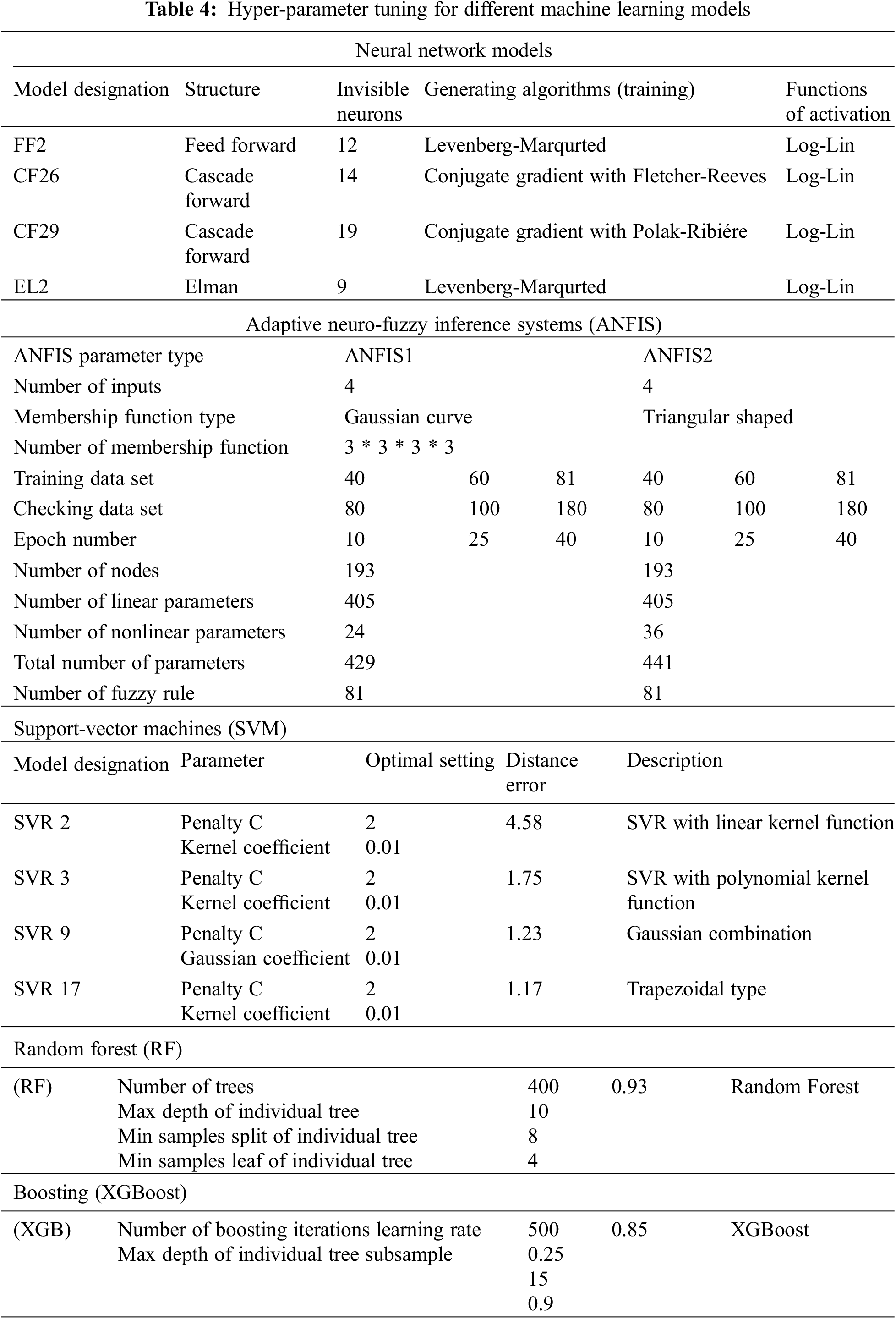
Figure 7: Results of testing by ANN models for: (a) Numerical model; (b) Experimental input data

ANN, ANFIS, SVM, RF and XGB (five separate machine learning approaches that employed equivalent prediction models for inputs and outputs data) findings were compared together. Those display data generated by experimental work taught with 70% of the data. Both the amount of computation required to produce predictions and the accuracy of the outcomes are included in the comparison. MATLAB2021b was used to develop, train, and test the models [19].

Several models’ performances were also assessed using a variety of statistical metrics, and the root-mean-square error (RMSE) was mostly used to improve the neurons in the hidden layer [20]:

Root mean square error (RMSE)=1N∑i=1N⁡(ai−pi)2 (7)

where N is the number of data sets, pi is the predicted value and ai is the experimental value.

Diverse membership function types were considered to determine the most appropriate models. A grid search among them revealed the type that yields the most accurate model for modelling various types that are selected based on input. With more membership functions per input, the computing effort needed to use the trained model for predictions increases exponentially. As a result, it was decided to simply select as we believed that the models illustrated in Table 5 dealt with accuracy sufficiently.

6.2 ANN Models

The most fundamental architecture of a neural network is the simple feed-forward neural network. There are three layers in this type. Each layer’s node is referred to as a neuron. The layer that is on top is the input layer. The two input neurons in Fig. 6 represent the two-dimensional input. The second layer contains the hidden layer while the bottom layer is the output layer. To estimate an output signal during the forward phase, the neurons are successively turned on from the input to the output layer. During the backward phase, the error is propagated through the network due to the discrepancy between the output signal and the correct value. This modifies the neuronal connection weights and reduces the probability of recurrent mistakes. To decide how much weight should change, optimization techniques such as Adam algorithm stochastic and gradient descent are used. To determine the gradient direction of each input weight, these techniques estimate the derivation of each neuron’s activation function.

To predict the fatigue life of the high-strength aluminum alloy 2090-T83, four ANN models feed-forward neural networks (FF2), cascade forward neural networks (CF26 and CF29), and Elman networks (EL2) are used and compared with the two traditional methods (input data with average values of the number of cycles ( Nf ) that were obtained from a numerical model and experimental input data with all obtained values). Exactly 10,000 trials were conducted to train the ANN, with each trial using between 9 and 19 random neurons in the hidden layer. The final ANN was picked because it handled experimental input with the least amount of inaccuracy. Twelve neurons made up the buried layer of the final ANN. The FF2, CF26, CF29 and EL2 models are used to predict fatigue life, as shown in Figs. 7a and 7b with numerical and experimental models vs. feed-forward neural network models.

Fig. 8 graphically compares the accuracy of ANN models to experimental and numerical input data.

Figure 8: Assessment of the produced ANN models’ accuracy and duration of the calculations

6.3 ANFIS Models

In this section, two models of ANFIS models were considered; one with fifth membership functions per input and the other with three membership functions per input (total of 72 and 800 rules, respectively). The algorithm shown in Fig. 9 was used to select the ideal kind of membership function. Triangle membership functions are employed in the most precise regression models for both the ANF1 and ANF2 models, according to the results of the grid search. Models with various Gaussian membership types were considered for selecting the best ANFIS results. A grid search was used to demonstrate that the triangular function creates the most precise model, producing both models with ANF1 and ANF2 per input. As the number of membership functions per input rises, the amount of computing needed to use the trained model for predictions grows exponentially. The model accuracy was deemed sufficient at two MFs per input and did not significantly increase with the addition of more MFs per input; therefore, it was chosen to stop there.

Figure 9: Algorithm for determining the appropriate hyper-parameter values for each model

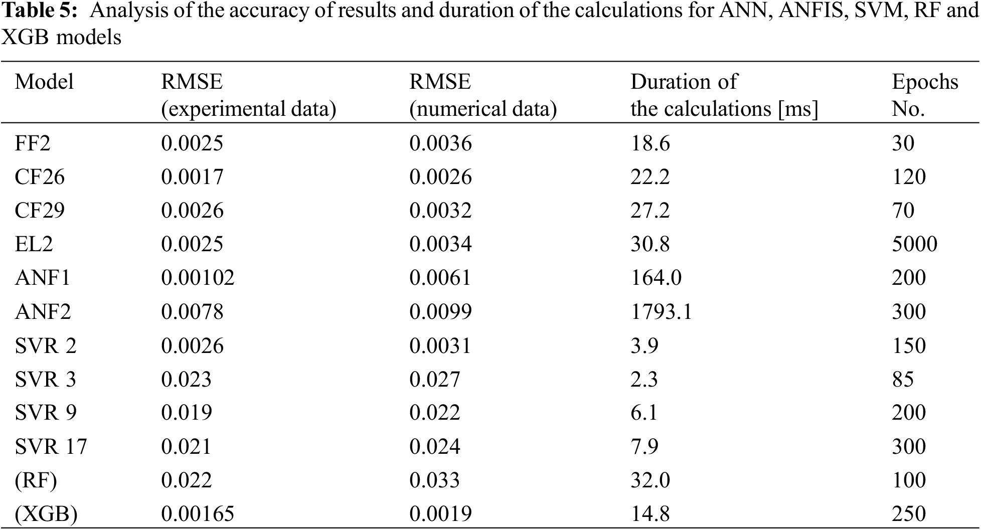
The effectiveness of the techniques developed using the algorithm is illustrated in Figs. 10 and 11. After applying the input data from numerical simulations and a series of experiments (average and all input data) based on measured levels of applied torsional stresses and determined for experimental inputs, the results were compared to reference data. The accuracy and amount of time needed to complete the calculations for the derived ANFIS models are listed in Table 5. The RMSE, which compares the model output to experimental data obtained through numerical simulations, is used to determine the accuracy. The duration of calculations for each point in the experimental input dataset is used to calculate the needed duration of calculations effort. The duration of calculations was determined using the MATLAB software’s average of 100 runs.

Figure 10: Algorithm for identifying the best models for each category

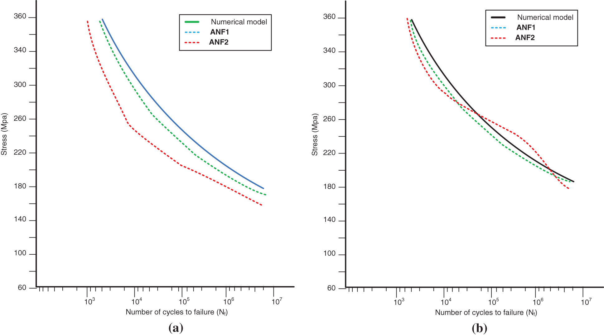
Figure 11: Results of testing by Adaptive neuro-fuzzy inference systems (ANFIS) for numerical input data (with average values of stresses): (a) ANFS1 (b) ANFS2

RMSE from experiments with data collected during tests is significantly more relevant than RSME with respect to digitally generated input data. Results for the ANF1 and ANF2 models are not significantly different (see Fig. 11). It is clear from the results (see Table 5) that ANF2 produces results with an RMSE greater than 8% while requiring approximately 11 times as much computing work as the ANF1 model, as shown in Fig. 12. So the ANF1 model will be used for further studies (Both RSME values are very slight), and the potential real-time applications of the ANF2 model raise concerns due to its high computing cost and lack of accuracy when compared to the ANF1 model.

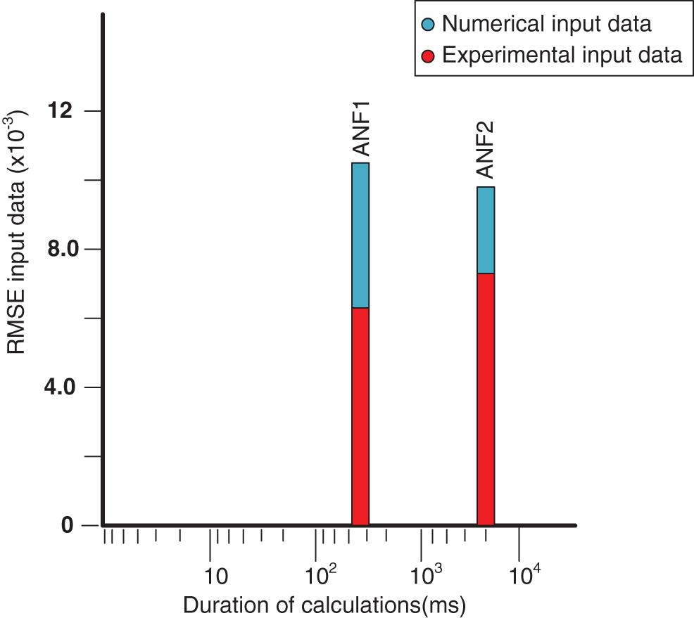
Figure 12: Assessment of the produced ANFIS models’ accuracy and duration of the calculations

6.4 Support-Vector Machines (SVM) Models

Fig. 10 is shown the produced four SVR 2, SVR 3, SVR 9 and SVR 17 models with the best hyperparameter values (out of 500 trials, each is the best). The models were evaluated using experimental and numerical input data, similar to the ANFIS models. Fig. 13 is represented the numerical and experimental results of the result of the support-vector machines (SVM) models test.

Figure 13: Results of testing by support-vector machines (SVM) models for: (a) Numerical model; (b) Experimental input data

The same metrics used for the ANFIS models were used to assess the accuracy and the necessary duration of calculations effort. Table 5 compares the four models, and Fig. 14 shows the graphical comparison of the accuracy of numerical and experimental input data. Fig. 13 demonstrates that the linear model provided somewhat erratic results when dealing with empirically observed inputs, despite having been trained on data that have white gauss noise added. The experimental input data were noisy, yet the gaussian model was shown to be the most stable (resistant). Since the SVR 9 has RMSE that is roughly three times smaller than the SVR 17 and all models require the same amount of time to compute, SVR 9 will be used for further analysis.

Figure 14: Assessment of the produced SVM models’ accuracy and duration of the calculations

Four different kernel functions were considered for SVM models. Grid searches of the hyperparameter values were used for all pertinent models. Gaussian kernel function (SVR 9) model outperformed the three other models in terms of accuracy by an order of magnitude. The SVM tests (see Fig. 13) illustrate that SVR 2 was not resistant to distorted experimental input data, even if all models were trained on numerical data with white gaussian noise added, and this is regarded as being of utmost importance. The SVM 9 model was chosen for further investigation even though it took longer to compute than the SVR 2, SVR 3, and SVR 17 models since the others, even when assessed, did not do well using numerical and experimental input data that was the same as that used in training.

6.5 Random Forest (RF) and Boosting (XGBoost) Models

One of the ensemble approaches, the RF algorithm, builds many regression trees and averages the final forecast from each tree’s results [21]. Gradient boosting’s fundamental idea is a simple technique for creating a new model in the direction of the residual errors in order to reduce the loss function that is produced at each iteration. Particularly in terms of scalability, parallelization, optimization, and accuracy, XGBoost demonstrates its supremacy [22].

For Random Forest (RF) and Boosting (XGBoost) techniques (based on Table 4) with various covariance methodologies, a grid search for a single hyper-parameter was carried out, where 75 and 100 logarithmically evenly spaced points, respectively, were produced. The algorithm shown in Fig. 10 was used to generate the final RF and XGBoost models while accounting for the best hyperparameter values discovered. The generated models’ S-N curves, derived for the same numerical and experimental input data as before, are shown in Fig. 15. As with the ANN, ANFIS and SVM models, Table 5 compares the precision and computing effort needed for the RF and XGBoost models. Fig. 16 provides a graphic representation of the same comparison for easier viewing.

Figure 15: Results of testing by Random Forest (RF) and XGBoost (XGB) models for: (a) Numerical model; (b) Experimental input data

Figure 16: Assessment of the produced RF and XGB models’ accuracy and duration of the calculations

The RF model’s output is less accurate than the XGB model’s when dealing with the numerical input data of the two models. But when compared to the experimental data, the XGB model was shown to be the most effective, producing 15%–25% more accurate findings than the other model and using the least amount of processing time. The RF model, which when applied to the empirically recorded input data, has an almost identical disposition, will be excluded from additional considerations even if the derived accuracies of the two models are good. This is evident in Fig. 16, where the XGB model outperforms the RF models in both studied criteria.

6.6 The Comparison between the ANN, ANFIS, SVM and XGB Models

The chosen ANN, ANFIS, SVM, and XGB models were compared with one another. The responses of the models to an empirically recorded and numerically generated S-N curve are shown in Fig. 17. Table 6 compares the computed root mean square errors with the actual a duration of the calculations. Fig. 18 displays a graphic comparison of the models’ precision (numerical and experimental input data) with duration of the calculations. The ANF1 was the most accurate and the XGB the most effective in terms of computation (about 20% less accurate than ANF1, but needing roughly 35 times less the duration of calculations). Given its inaccuracy and computational complexity, the SVR 9 model was the worst performer among all those evaluated. The accuracy of the CF26 model was quite comparable to that of the SVR 9 (8% best), but it was four times slower.

Figure 17: Results of testing selected models of various techniques: (a) Numerical input data; (b) Experimental input data

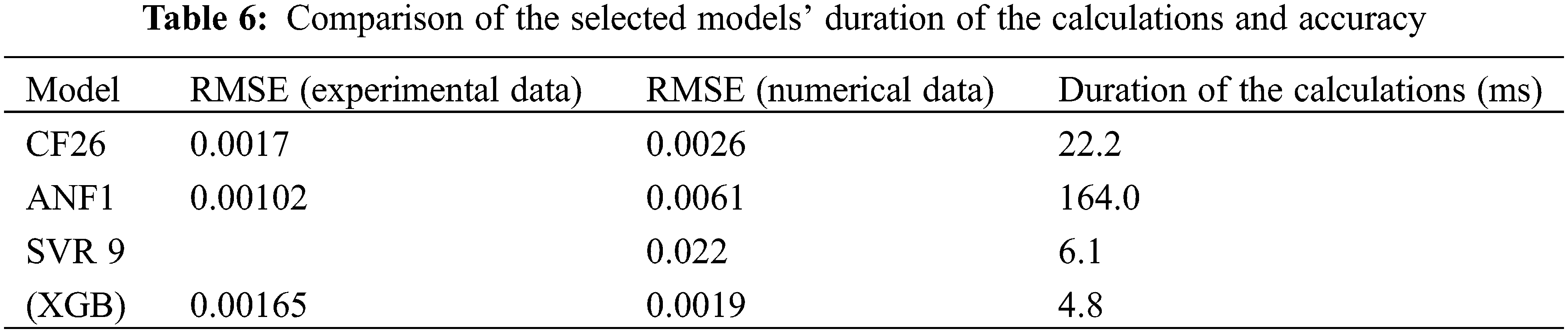
Figure 18: A graphic comparison of the duration of the calculations and accuracy for the models that were chosen

7  Concluding Remarks

Under pure torsion loading induced with various applied stresses, the fatigue life of the high strength aluminum alloy 2090-T83 was predicted using different types of machine learning approaches (ANN, ANFIS, SVM, RF, and XGB). The accuracy and time required for the computations were evaluated by comparing the findings to one another. The following conclusions were reached:

1.    Considering the aforementioned findings, it is concluded that, for all activation functions and training procedures, forward neural network models outperform traditional methods.

2.    The accuracy of the CF26 neural network’s findings when compared to all models used in ANNs and, in most cases, the additional weight employed in these networks, which could improve the network’s accuracy, make it evident from these results that the CF26 produces strong results.

3.    Various forms of membership function modelling techniques were considered to find the ideal ANFIS with one or two membership functions for each entry, as it was found that two membership functions for each input data did not significantly improve them, and therefore, stopping at one MFs was determined for each entry.

4.    Four different kernel functions were considered for SVM models (SVR 2, SVR 3, SVR 9 and SVR 17). Grid searches of hyperparameter values were done for all four models. The gaussian kernel function (SVR 9) model outperformed the other models in terms of accuracy by an order of magnitude.

5.    With various covariance functions, random forest (RF) and tree boosting (XGBoost) models were taken into consideration. Their results for calculation time and accuracy were very different from one another.

6.    For the final comparison, the best model from each of the above categories, namely CF26, ANF1, SVR 9 and XGB, was selected. The accuracy of each specific model was distinct, acceptable, and consistent in scale. However, it was found that the resulting model from XGB gives better accuracy and acceptable computational time compared to the rest of the models.

7.    The experimental input interacts with the above-mentioned training models that were adopted in this research more effectively when compared with the numerical model.

For fatigue field, one should consider two methods—ANF1 and GBX. The GBX model is the fastest due to simple floating-point operations in each layer; however, finding the accurate model could be hard or even impossible. In this case, the ANF1 model could be easier to implement, as it was proven to have good repeatability.

Acknowledgement: The authors would like to thank the Department of Electromechanical Engineering at the University of Technology in Baghdad, Iraq for its contribution in support to carry out this research.

Funding Statement: The authors received no specific funding for this study.

Conflicts of Interest: The authors declare that they have no conflicts of interest to report regarding the present study.

References

1. Chen, J., Liu, Y. (2022). Fatigue modeling using neural networks: A comprehensive review. Fatigue & Fracture of Engineering Materials & Structure, 45(4), 945–979. [Google Scholar]

2. Abdullatef, M. S., AlRazzaq, N., Hasan, M. M. (2016). Prediction fatigue life of aluminum alloy 7075 T73 using neural networks and neuro-fuzzy models. Engineering and Technology Journal, 34, 272–283. [Google Scholar]

3. Barbosa, J. F., Correia, J. A., Júnior, R. F., de Jesus, A. M. (2020). Fatigue life prediction of metallic materials considering mean stress effects by means of an artificial neural network. International Journal of Fatigue, 135, 105527. [Google Scholar]

4. Dharmadhikari, S., Basak, A. (2022). Fatigue damage detection of aerospace-grade aluminum alloys using feature-based and feature-less deep neural networks. Machine Learning with Applications, 7, 100247. [Google Scholar]

5. Mohanty, J. R., Verma, B. B., Parhi, D. R. K., Ray, P. K. (2009). Application of artificial neural network for predicting fatigue crack propagation life of aluminum alloys. Computational Materials Science and Surface Engineering, 1(3), 133–138. [Google Scholar]

6. Himmiche, S., Mortazavi, S. N. S., Ince, A. (2021). Comparative study of neural network-based models for fatigue crack growth predictions of small cracks. Journal of Peridynamics and Nonlocal Modelling, 4(4), 1–26. [Google Scholar]

7. Bentéjac, C., Csörgo, A., Martínez-Muñoz, G. (2019). A comparative analysis of XGBoost. arXiv:1911.01914. [Google Scholar]

8. Basak, D., Pal, S., Patranabis, C. D. (2007). Support vector regression. Statistics and Computing, 11(10), 203–224. [Google Scholar]

9. Branco, R., Martins, R. F., Correia, J. A. F. O., Marciniak, Z., Macek, W. et al. (2022). On the use of the cumulative strain energy density for fatigue life assessment in advanced high-strength steels. International Journal of Fatigue, 164, 107121. [Google Scholar]

10. Macek, W., Robak, G., Zak, K., Branco, R. (2022). Fracture surface topography investigation and fatigue life assessment of notched austenitic steel specimens. Engineering Failure Analysis, 135, 106121. [Google Scholar]

11. Abdullatef, M. S., AlRazzaq, N., Abdulla, G. M. (2017). Prediction of fatigue life of fiber glass reinforced composite (FGRC) using artificial neural network. Engineering and Technology Journal, 35. https://doi.org/10.30684/etj.35.4A.4 [Google Scholar] [CrossRef]

12. Garg, B., Kumar, P. (2007). Fatigue behaviour of aluminium alloy (MSc. Thesis). National Institute of Technology, Rourkela. [Google Scholar]

13. Boyer, H. E. (1986). Fatigue testing. In: Atlas of fatigue curves, 6th edn, pp. 1–10. ASM International. [Google Scholar]

14. Nechval, K. N., Nechval, N. A., Bausova, I., Šķiltere, D., Strelchonok, V. F. (2006). Prediction of fatigue crack growth process via artifitial neural network technique. International Scientific Journal of Computing, 5(3), 1–12. [Google Scholar]

15. Awodele, O., Jegede, O. (2009). Neural networks and its application in engineering. Proceedings of the Informing Science & IT Education Conference (InSITE), vol. 9, pp. 83–95. Macon, GA, USA. [Google Scholar]

16. Mentes, A., Yetkin, M., Kim, Y. (2016). Comparison of ANN and ANFIS techniques on modeling of spread mooring systems. Proceedings of the 30th Asian-Pacific Technical Exchange and Advisory Meeting on Marine Structures (TEAM 2016) Mokpo, pp. 252–258. Korea. [Google Scholar]

17. Material Property Data (MatWeb). https://www.matweb.com/index.aspx [Google Scholar]

18. AVERY Fatigue Testing Machine. User’s instructions 7305. [Google Scholar]

19. MathWorks Introduces Release 2021b of MATLAB and Simulink. https://uk.mathworks.com/company/newsroom/mathworks-introduces-release-2021b-of-matlab-and-simulink.html [Google Scholar]

20. Hasan, M. M. (2015). Prediction fatigue life of aluminum alloy 7075−T73 using neural networks and neuro-fuzzy models (MSc. Thesis). University of Technology, Iraq. [Google Scholar]

21. Joharestani, M. Z., Cao, C., Ni, X., Bashir, B., Talebiesfandarani, S. (2019). Prediction based on random forest, XGBoost, and deep learning using multisource remote sensing data. Atmosphere, 10(7), 373. https://doi.org/10.3390/atmos10070373 [Google Scholar] [CrossRef]

22. Lee, C., Lee, S. (2022). Exploring the contributions by transportation features to urban economy: An experiment of a scalable tree-boosting algorithm with big data. Land, 11(4), 577. https://doi.org/10.3390/land11040577 [Google Scholar] [CrossRef]

Appendix A