Numerical Investigation of Load Generation in U-Shaped Aqueducts under Lateral Excitation: Part I—First-Order Resonant Sloshing

1 Introduction

Regions with high seismic activity account for a significant portion of strong earthquakes worldwide. Statistics indicate that approximately 35% of earthquakes with a magnitude of 7 or higher occur in seismically active areas [1]. As an overhead water diversion structure spanning rivers and other obstacles, aqueducts are critical hydraulic facilities in water diversion projects. During operation, the mass of water inside an aqueduct often exceeds that of the structure itself. The complex fluid-structure interaction between the water and the aqueduct significantly affects the dynamic characteristics and response of the aqueduct [2].

In recent decades, several countries have constructed or planned a large number of major water diversion projects. Consequently, extensive research has been carried out on aqueducts. Existing studies on the dynamic response of aqueducts under transverse seismic excitation present two conflicting perspectives: (1) Some scholars argue that when the resonance frequency of the water is close to the natural frequency of the overall structure, the water will absorb part of the vibration energy, leading to a reduction in the vibration amplitude of the aqueduct. Thus, the water more or less plays the role of a Tuned Liquid Damper (TLD) (e.g., Refs. [3,4,5]). (2) Due to the fluid-structure interaction between the water and the aqueduct, the presence of water tends to amplify the dynamic response of the aqueduct structure (e.g., Refs. [6,7]). In summary, most studies on the dynamic response of aqueduct structures under transverse seismic excitation have not reached a consistent conclusion.

On one hand, in recent years, the application of various forms of TLDs in structural vibration suppression has been a hot topic in research. Many scholars have carried out numerical simulations and model tests in this field. For example, Ocak et al. applied the adaptive harmony search algorithm (AHS) to optimize the use of TLDs with different liquids on single-story, ten-story, and forty-story building models. The results showed that the optimized TLD can significantly reduce structural displacement and total acceleration, thereby enhancing the seismic performance of buildings, and that the optimal liquid choice varies for different building models [8]. Yusuf et al. combined experimental and numerical analysis methods, utilizing the Ansys Fluent to investigate the vibration control of wind turbine towers. The results showed that a single TLD (with a mass ratio of 4%) could reduce the lateral displacement of the tower by 7.32%, while three TLDs (with a mass ratio of 12%) could reduce it by 48.73% [9]. He et al. employed computational fluid dynamics (CFD) methods and conducted secondary development using OpenFOAM to establish a two-way coupled numerical model. This model was used to study the nonlinear liquid sloshing characteristics of TLDs and their performance in wind-induced vibration control of high-rise buildings. The results indicated that TLDs can effectively mitigate the vibration response of single-degree-of-freedom (SDOF) rigid frame structures under harmonic excitation. At resonance excitation, the maximum displacement response of the structure could be reduced by as much as 78.5% [10]. Domizio et al. proposed a novel high-frequency tuned liquid damper (HF-TLD) and studied its effectiveness in controlling high-frequency structural vibrations through experimental and theoretical analysis. Experimental results demonstrated that the HF-TLD could respond effectively in a wide frequency range above 2.5 Hz and effectively control the dynamic response of low-rise or high-natural-frequency structures. At a mass ratio of 5%, the HF-TLD reduced the maximum relative displacement of the structure by an average of about 20% [11]. Sun et al. investigated the seismic performance of a novel tuned liquid damper with a damping net and a sloped-bottom (DNS-TLD) through mechanical modeling, simplified equivalent damping estimation, single-frame shaking-table tests and numerical simulation. They concluded that DNS-TLD outperforms conventional TLDs in damping capacity, efficiency, robustness and applicability while using less water, thus offering an effective tool for real structural seismic control [12]. Zhou et al. used CFD-coupled simulation and particle swarm optimization to study optimal design of multiple tuned liquid dampers with paddles for mitigating wind-induced vibrations of a 206 m tall building. They concluded that the proposed multi-frequency optimization markedly improves robustness against structural frequency shift, achieving 28–33% better damping performance than traditional single-frequency tuning [13]. Xue et al. used a bidirectional fluid-structure coupling model validated by lab experiments to study tuned liquid column damper (TLCD) vibration control on offshore platforms. They found optimal mass ratio of water-to-platform at 1.5%, tuning ratio at 1.0, achieving up to 78% displacement reduction while avoiding frequency detuning [14]. Saghi and Zi numerically studied a barge-type floating offshore wind turbine (FOWT) integrated with a bidirectional tuned liquid damper (BTLD) using OpenFOAM. They optimized BTLD geometry and placement to reduce pitch motion. Results showed that an optimal BTLD can reduce pitch motion by 10–30%, with the best configuration decreasing pitch by up to 34% at the natural period [15]. Saghi et al. used CFD-RANS/VOF coupled overset-mesh simulations in OpenFOAM to study bidirectional tuned liquid damper (BTLD)/bidirectional tuned liquid column damper (BTLCD) effectiveness on barge-type and octagonal FOWTs under wave loads. They concluded optimal BTLD (case 9, 4 m baffle) and BTLCD (case 6, 60% opening) integrated with 6 m-corner octagonal substructures achieve maximum 28% pitch-motion reduction, while BTLD offers wider damping bandwidth than BTLCD [16]. Liao et al. employed nonlinear finite-element (CEL) modeling and dual-performance optimization to investigate a new baffle-isolated tuned liquid damper (NDB-ITLD). They found that bottom vertical baffles plus elastomeric isolation markedly widen control bandwidth, enhance energy dissipation, and simultaneously cut both structural displacement and isolation-layer deformation under diverse seismic intensities [17].

On the other hand, the water sloshing in aqueducts is essentially a sloshing problem of water in liquid storage containers. Regarding liquid sloshing in containers, Akyildiz and Ünal investigated the pressure variations and three-dimensional effects of water sloshing in rectangular containers through physical experiments. They found that baffles significantly reduce pressure fluctuations, especially under shallow water cases, and that excitation amplitude and frequency have a notable impact on impact pressure [18,19]. Liu and Lin established a numerical model to study nonlinear sloshing in rectangular containers, employing the Large Eddy Simulation (LES) method to model turbulence effects and a second-order accurate VOF method to capture breaking free surfaces. Their results showed that numerical solutions align with linear theory under small excitations and match experimental data under large excitations, validating the capability of their model to simulate breaking free surfaces and strong turbulence [20]. Elahi et al. used a two-dimensional numerical model with the VOF method to capture free surface motion, studying the effects of free surface displacement, fluid viscosity, and surface tension on liquid sloshing in containers. Their results indicated that the model accurately simulates liquid sloshing under complex excitations, including linear, rotational, and coupled motions, providing an effective numerical tool for analyzing sloshing problems [21]. Tosun et al. combined image processing techniques with potential flow theory to study liquid sloshing characteristics in rectangular tanks, including free surface tracking and sloshing force estimation. Their results demonstrated that this method accurately estimates free surface shapes and sloshing forces near resonance frequencies without the need for traditional force sensors [22]. Jin and Lin used numerical methods to investigate the effects of fluid viscosity on liquid sloshing in three-dimensional rectangular containers. They found that viscosity significantly influences free surface behavior, pressure response, rising time, and frequency response, and identified a critical viscosity value that shifts the response from natural frequency to external excitation [23]. Cai et al. compared the VOF, Smoothed Particle Hydrodynamics (SPH), and Arbitrary Lagrangian-Eulerian (ALE) methods to study rigid body forces in partially filled sloshing tanks, recommending SPH and VOF models as superior choices [24]. Jiang et al. developed and validated a three-dimensional variable-mass tank sloshing model using numerical simulations. Their results showed that refueling increases liquid mass, suppressing sloshing but increasing loads, with loads rising as refueling rates increase. Baffles were found to effectively suppress sloshing [25].

To sum up, In the field of TLD, studies mainly focus on three aspects: developing new TLD devices (e.g., Refs. [11,12,17]), analyzing TLD’s seismic mitigation effects on specific structures (e.g., [9,10,14]), and optimizing TLD designs (e.g., Refs. [8,13,15]). In the field of liquid sloshing in containers, existing studies primarily focus on the improvement and comparison of numerical simulation methods (e.g., Refs. [18,19,20]), sloshing characteristics under complex excitations (e.g., Ref. [25]), the effects of viscosity, and engineering applications (e.g., Refs. [22,23]). However, both fields lack systematic research on the generation mechanism of sloshing loads. This scientific gap is particularly significant for gaining a deeper understanding of the dynamic response of aqueduct structures and for developing seismic mitigation devices for these structures. As a typical large mass ratio liquid-structure coupled system, the water-structure mass ratio of an aqueduct (usually 1:3) is much higher than that of conventional TLD devices. Although the spring-mass equivalent model is commonly used in current engineering practice for aqueduct seismic analysis, it can only meet basic design requirements and cannot reveal the coupling mechanism between liquid sloshing and structural dynamic responses. The inertial forces and impact loads generated by liquid sloshing may dominate the dynamic response of aqueduct structures, and their mechanisms are fundamentally different from conventional TLD.

To deeply analyze the dynamic response of aqueducts under seismic action, it’s essential to understand the morphological changes of water inside aqueducts during earthquakes and to reveal the generation mechanisms of sloshing forces acting on the inner walls of aqueducts. This can also provide new insights into sloshing load generation for other fields, such as TLD research and liquid sloshing in containers studies. The U-shaped aqueduct, commonly used in water diversion projects, is selected as the research object. Two-dimensional (2D) Computational Fluid Dynamics (CFD) models for the fluid domain of U-shaped aqueduct are established by ANSYS Fluent, and a set of harmonic displacements with different amplitude and frequency are employed to simulate seismic action. In this study, the generation mechanisms of sloshing forces during the first-order transverse resonance of water in a 2D U-shaped aqueduct are investigated. The mechanisms leading to the extreme and zero values of the horizontal force F h and the fluctuating component of the vertical force F v f are analyzed, along with the influence of free surface fluctuations on pressure distribution. Additionally, the conversion between potential energy and kinetic energy of the water inside the aqueduct is examined.

2 Numerical Model

2.1 Geometric Model

A simply supported aqueduct with a U-shaped cross-section, commonly used in water diversion projects, is selected as the research object in this study. The dimensions of the cross-section of this aqueduct are shown in Fig. 1 below.

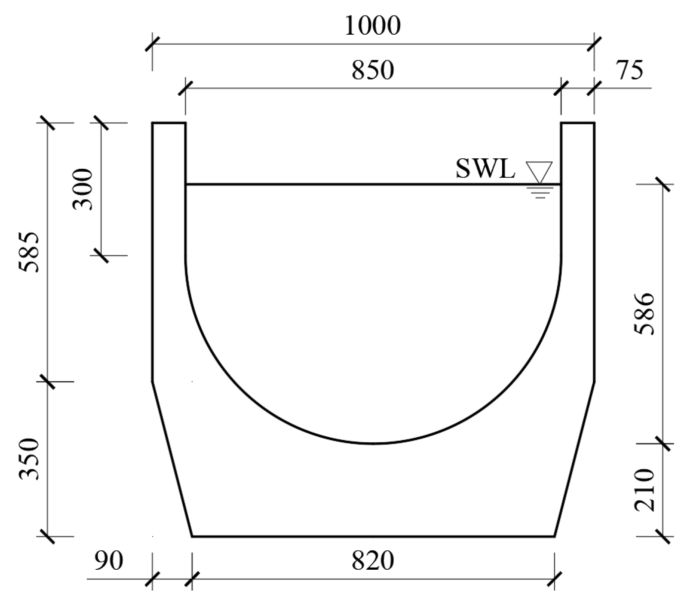
Figure 1: Dimensions of cross-section of the aqueduct used in this study (units: cm).

When simulating the transverse vibration of the water in the aqueduct, the fluid domain can be directly simplified into two dimensions. To increase the difficulty of water escape during high-frequency sloshing (i.e., the escape of water is not considered in this study by employing the following method), the 2D numerical model used in this study extends the side walls by 3 m based on Fig. 1. The specific dimensions of fluid domain are shown in Fig. 2. The upper boundary of the U-shaped fluid domain is set as a pressure outlet (indicated by the black dash dot line in Fig. 2), while all remaining boundaries are defined as no-slip walls. Due to the symmetry of the U-shaped fluid domain, the walls in the numerical model are divided into left and right parts (as shown in Fig. 2). The pressure distribution along the no-slip walls is monitored in Ansys Fluent. In this study, when describing the physical fields of the fluid inside the aqueduct obtained from the numerical model, an absolute coordinate system (fixed coordinate system) is employed by Ansys Fluent for representation. The absolute coordinate system is established at the Origin (0, 0), as illustrated in Fig. 2.

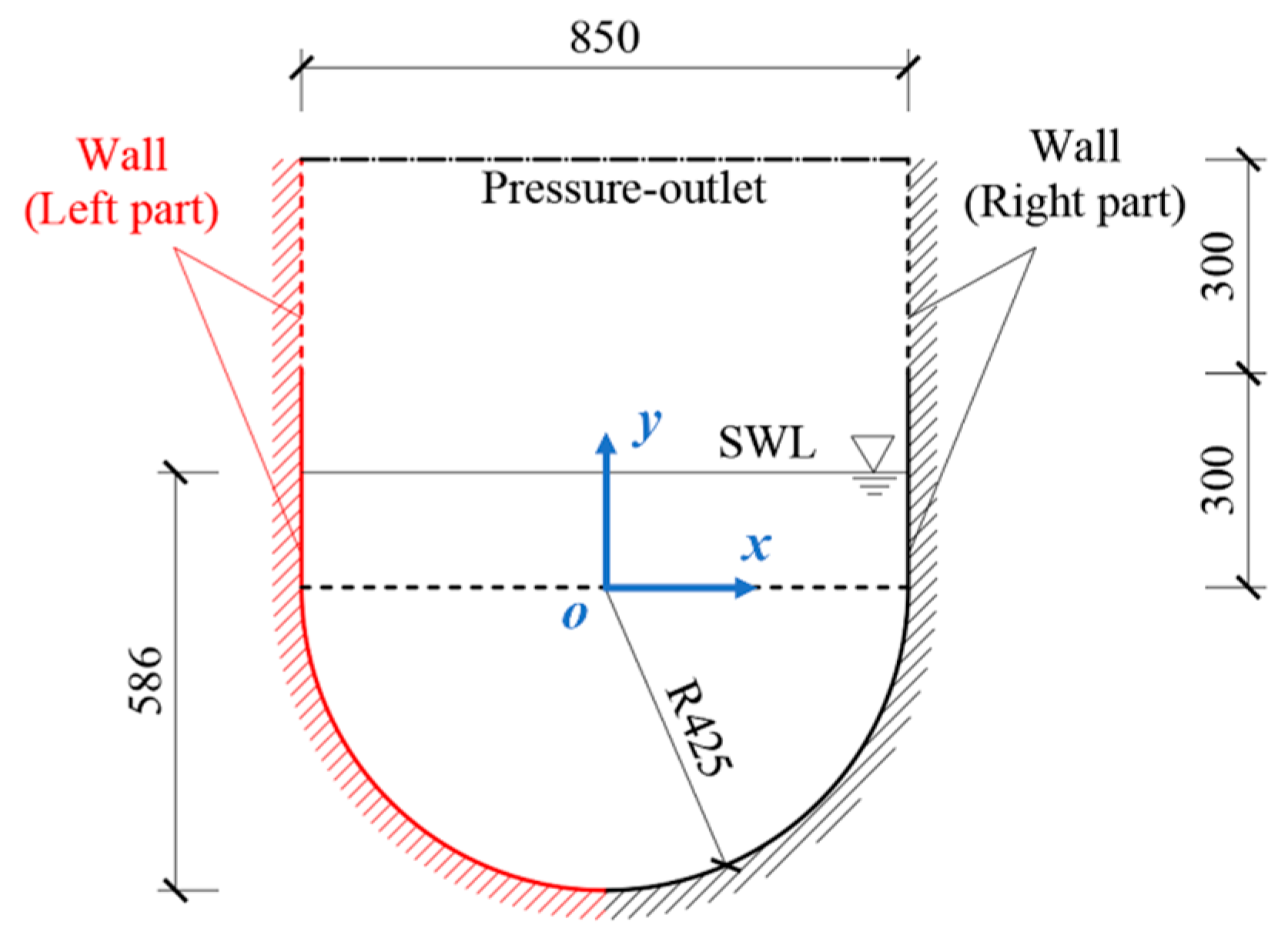
Figure 2: Dimensions of the 2D CFD model of the fluid domain inside the aqueduct (extended side walls indicated by dash lines), wall segmentation method, and schematic of the body-fitted coordinate system (units: cm).

During the transient numerical simulation, the following time histories of different physical quantities are monitored: (1) The horizontal displacement of the fluid domain d t , and its derivatives, including the velocity u t and the acceleration a t . (2) The free surface fluctuation at the left and right walls of the aqueduct, i.e., h L t and h R t , respectively, and their derived quantity, the free surface difference inside the aqueduct Δ h t = h R t − h L t . (3) The resultant forces on the inner walls of the aqueduct, including the horizontal force F h t and vertical force F v t . (4) The pressure distributions on the inner walls of the aqueduct, including static pressure p s t a t i c t , dynamic pressure p d y n a m i c t , and total pressure p t o t a l t .

To eliminate the influence of different dimensions and more directly reflect the phase relationships among the physical quantities mentioned above, normalization is performed according to Eq. (1). Each physical quantity is remapped to the range [−1, 1]. ϕ¯t=ϕtϕmax,(1) where, ϕ ¯ t represents a time history of any physical quantity undergoing normalization (e.g., d t , u t , a t , Δ h t ), ϕ ¯ t is the normalized time history, and ϕ m a x is the maximum absolute value of ϕ t over a specified range.

Since F v t does not oscillate around zero, only its fluctuating component is normalized in this study. The fluctuating component of F v t can be calculated as follows: Fvft=Fvt−Fv−static,(2) when water depth inside the aqueduct is constant (5.86 m), the vertical force exerted by the water on the aqueduct in a static state is F v − s t a t i c = − 411.26 kN.

2.2 Numerical Cases

In this study, harmonic displacement is used to analyze the generation mechanism of sloshing forces during transverse vibration of the water in the aqueduct. To determine the range of amplitude and frequency for the harmonic displacement used in this study, six real seismic displacement time histories were randomly selected from Pacific Earthquake Engineering Research Center (PEER). Their Peak Ground Displacement (PGD) and dominant frequency ranges are statistically analyzed, as listed in Table 1 below.

From Table 1, it can be observed that the PGD of all the selected ground motion records is generally within 10 cm. Therefore, harmonic displacements of 3 cm, 5 cm, 10 cm, and 15 cm are considered in this study. The dominant frequencies of the selected ground motion records in Table 1 are all smaller than 2 Hz. According to the study by Dou et al. [26], the first two transverse natural frequencies of the water (the first-order and third-order natural frequencies) in the U-shaped fluid domain (shown in Fig. 2) are 0.296 Hz and 0.524 Hz, respectively, which indicates that this first two transverse natural frequencies of the water fall within the dominant frequency range of the selected ground motion records.

Thus, a set of harmonic displacements with frequencies below 2 Hz is used to simulate the transverse vibration of the water in the U-shaped aqueduct. The amplitudes and frequencies of the harmonic displacements used in this study are listed in Table 2.

In this study, the cases are named in the format “Case A-f”, for example, “Case 0.03–0.2”, which indicate that the case of harmonic excitation with amplitude 0.03 m and frequency 0.2 Hz.

2.3 Validation for Numerical Simulation

Due to the large cross-sectional dimensions of the aqueduct selected in this study, physical experiments to validate the accuracy of the full-scale numerical model are impractical. And in the existing studies, there are only data on liquid sloshing in rectangular containers, and no studies have chosen a U-shaped container as the research object. We believe that the container shape has little influence on meshing method of the fluid domain, the various model settings in CFD software, boundary conditions, and model parameter settings. Therefore, a scaled-down rectangular container with dimensions of 30 cm × 30 cm × 30 cm (wall thickness: 0.5 cm, fluid domain: 29 cm × 29 cm × 29 cm) is used to verify the rationality of settings in Ansys Fluent. This validation aims to determine the optimal turbulence model and temporal resolution (time step size) for simulating liquid sloshing phenomena. Subsequently, the validated turbulence model and time step size are applied to the U-shaped aqueduct cross-section (as shown in Fig. 2) to perform grid independence validation.

To improve the convergence of the numerical model and reduce the influence of the initial sloshing state on subsequent processes, a gradual amplitude increase method with constant frequency is adopted. The excitation method for the numerical model is described as follows (The excitation method employed in the physical experiments is consistent with this): yt=0t≤0.5st−43fAsin2πft−40+0.5<t≤3f+0.5Asin2πft−43f+0.5<t≤7f+0.5,(3) where y t represents the real-time position of the fluid domain.

2.3.1 Governing Equations for Fluid Dynamics

The two-dimensional CFD model used in this study is established in ANSYS Fluent. The finite volume method (FVM) is employed to solve the incompressible Reynolds-Averaged Navier–Stokes (RANS) equations. The computational domain consisted of water and air, and the Volume of Fluid (VOF) method was adopted to capture the free surface between the two phases [27]. Pressure–velocity coupling was handled using the PISO algorithm, while the gradient was calculated using the least-squares cell-based scheme, pressure was interpolated with the PRESTO! scheme, and the momentum equations were discretized using a second-order upwind scheme [28]. For the volume fraction, a compressive scheme was applied to sharpen the interface [28]. The turbulence kinetic energy and dissipation rate were discretized with a first-order upwind scheme [28]. Temporal discretization was performed with a first-order implicit scheme [28]. The time step size was chosen such that the Courant number always remained below 0.5, thereby ensuring numerical stability and accuracy of the transient simulations.

Das et al. compared the computational precision of inviscid flow and six different turbulence models based on experimental data while studying the vibration suppression effect of Tuned Liquid Dampers (TLDs) on high-rise buildings by numerical simulation [29]. The six turbulence models include the Standard k - ε model, RNG k - ε model, Realizable k - ε model, Standard k - ω model, BSL k - ω model, and SST k - ω model. The results showed that the computational error between numerical simulations and experimental data was significant when inviscid model was employed, while the error was smaller when turbulence models were applied. Therefore, the RNG k - ε turbulence model is selected for this study, and its detail could be referred to Ref. [30].

2.3.2 Physical Experiment for Validation of Ansys Fluent Settings

The physical experiments were conducted in a laboratory equipped for structural and hydraulic testing. Six-component load cell from FORCECHINA named FC6D90 was used to measure the sloshing force. The measuring range of forces F x , F y and F z were 1000 N, 1000 N and 2000 N, respectively. The sampling frequency of the load cell was set as 200 Hz. The installation of the physical experiments is shown in Fig. 3. The total mass m of the empty tank and the flange plate is 5.23 kg.

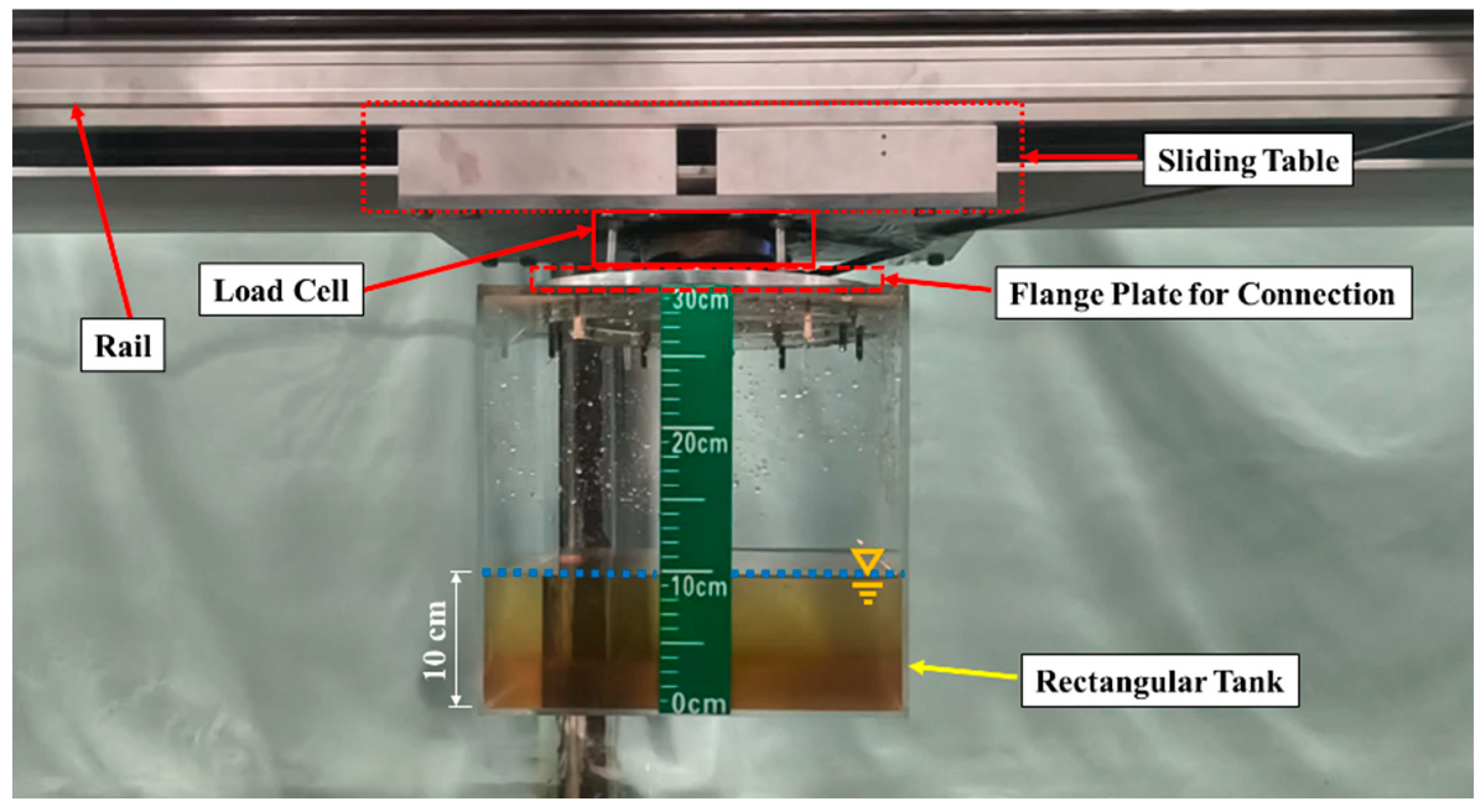
Figure 3: Photo of installation of the physical experimental model.

Based on the assumption of potential flow theory, the natural frequencies of water inside a rectangular tank can be analytically determined as [31], f=12πgπnLtanhπnLh,n=1,2,3,(4) where n is the mode number and h is the filling level. According to Eq. (4), the first-order natural frequency is f 1 = 1.46 Hz for the tank with 10 cm filling level, as shown in Fig. 3.

Prior to the official beginning of the experiment, no-load tests on the empty tank are conducted using a set of sinusoidal displacements with amplitude A = 0.003 m and frequencies of f = 1.1 Hz, 1.2 Hz, 1.3 Hz, 1.4 Hz, 1.5 Hz, 1.6 Hz, 1.7 Hz. This is done to verify the accuracy of the experimental data acquisition system. Table 3 presents the following results for each excitation case: the average of maximum values per cycle of the horizontal force during the stable segment F h − m a x a v g , the total mass of the model m e calculated by Newton’s second law, the error E m = 100 % × m e − m / m between the actual mass m and the calculated mass m e .

The data in Table 3 shows that the maximum error between the model mass m e derived from F h − m a x a v g and the actual model mass m is 7.52%, with an average error of 5.24%. Thus, the data obtained from the physical experiments in this study can be considered accurate.

In this section, the CFD model setup is verified using the first-order resonance case of water in a rectangular container (Case 0.003–1.46). Existing studies (e.g., Refs. [20,32,33]) have shown that uniform grids (with grid sizes corresponding to 1% of the width of the fluid domain) are sufficient for numerical simulations of liquid sloshing in storage containers and similar problems, and 2D CFD model is precision enough to simulate the liquid sloshing in 3D rectangular tanks under horizontal excitations. Therefore, a 2D CFD model ( 0.29 m × 0.29 m ) is established in Ansys Fluent with grid sizes of 0.0029 m . Based on this 2D numerical model, three different number of time step (10,000, 5000, and 2000) and two different turbulence model (laminar and RNG k - ε model), totally 6 cases, are compared with experiment data to determinate the rationality of each setting in Ansys Fluent.

The time-history curves of horizontal force F h from six numerical models and physical experiments during two cycles of stable segment are shown in Fig. 4. F h − m a x a v g from six numerical models and physical experiments, and the errors of F h − m a x a v g ( E = 100 % × F h − m a x a v g n u m − F h − m a x a v g e x p / F h − m a x a v g e x p ) between six numerical models and physical experiments are listed in Table 4.

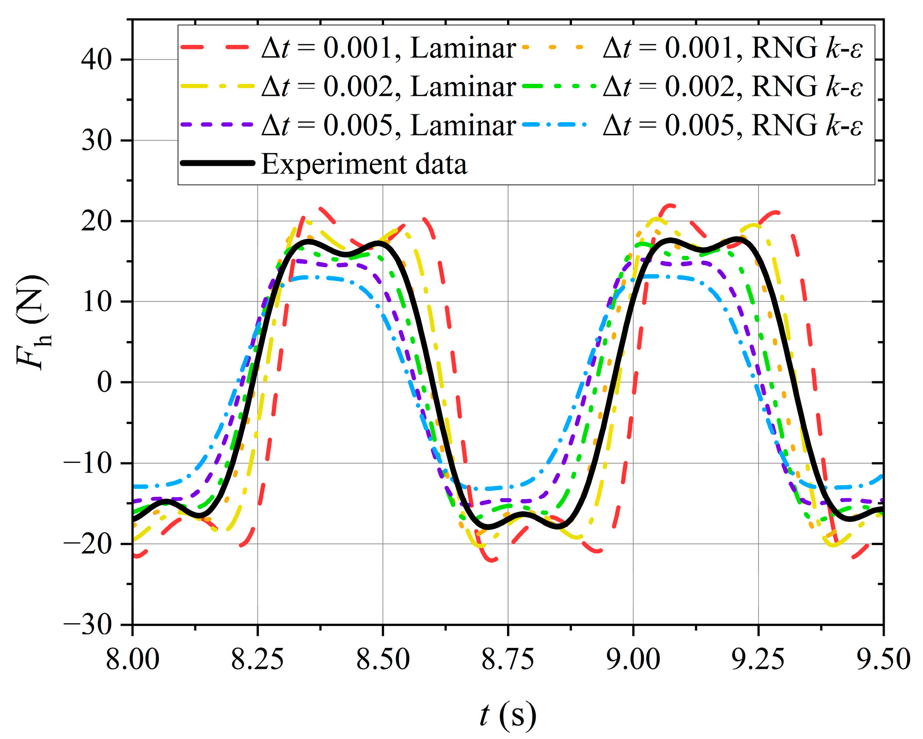
Figure 4: The time history curves of the horizontal force F h generated by 6 numerical models and experiments during two cycles in the stable segment. Note that the time history curve obtained from the experiment has eliminated the influence of model mass.

From the time-history curve of the physical experiment in Fig. 4, it can be seen that the curve has the characteristic of two peaks. Except for the two models with Δ t = 0.005 , the other four models have captured this characteristic of the time-history curve. Although there are differences in the peak values of the horizontal force calculated by each model, this study mainly focuses on the generation mechanism of liquid sloshing loads, and the influence of the peak values of the time-history curve can be ignored. From the F h − m a x a v g obtained by each model in Table 4 and its error analysis, it can be known that the time history curve of the horizontal force F h obtained by the Model 5 ( Δ t = 0.005 s , RNG k - ε model) is in the best agreement with the data obtained by the physical experiments. Therefore, in this study, the excitation process shown in Eq. (3) will be uniformly divided into 5000 time steps for simulation, and the RNG k - ε model will be selected as the turbulence model.

2.3.3 Grid Independence Test

For the grid independence test, six different schemes of grids are selected, with grid sizes corresponding to 0.5%, 0.625%, 0.75%, 0.875%, 1%, and 2% of the width of the U-shaped fluid domain. The basic information of these grids, as well as the average of maximum values per cycle of the horizontal force, the fluctuating component of the vertical force ( F h − m a x a v g and F v f − m a x a v g ) under the Case 0.05–0.296 and the Case 0.05–1.8, are listed in Table 5 and Table 6, respectively. The errors of F h − m a x a v g and F v f − m a x a v g obtained from the 0.625%, 0.75%, 0.875%, 1%, and 2% grids, relative to the 0.5% grid, as shown in Eq. (5), are also provided in Table 5 and Table 6, respectively. E∗S=F∗S−F∗0.5%F∗0.5%×100(5) where ∗ represents F h − m a x a v g or F v f − m a x a v g . S represents the scheme of the grids (e.g., 0.5%, 0.625%, 0.75%, …).

According to the results in Table 5 and Table 6, except for the 2% grid, the E F h − m a x a v g S for other grid sizes is less than 1%, and the E F v f − m a x a v g S is less than 5%. Thus, the results can be considered independent of mesh size. Considering computational efficiency and precision, 1% grid is selected for use in this study eventually.

3 Results of Numerical Simulation

Among all the non-resonance cases, the time history curves of F h and F v exhibit consistent characteristics. Specifically, the segment 0 ~ 0.5 + 3 f is unstable, while the segment 0.5 + 3 f < t ≤ 7 f + 0.5 is stable, as the amplitude of the excitation no longer changes, as shown in Fig. 5.

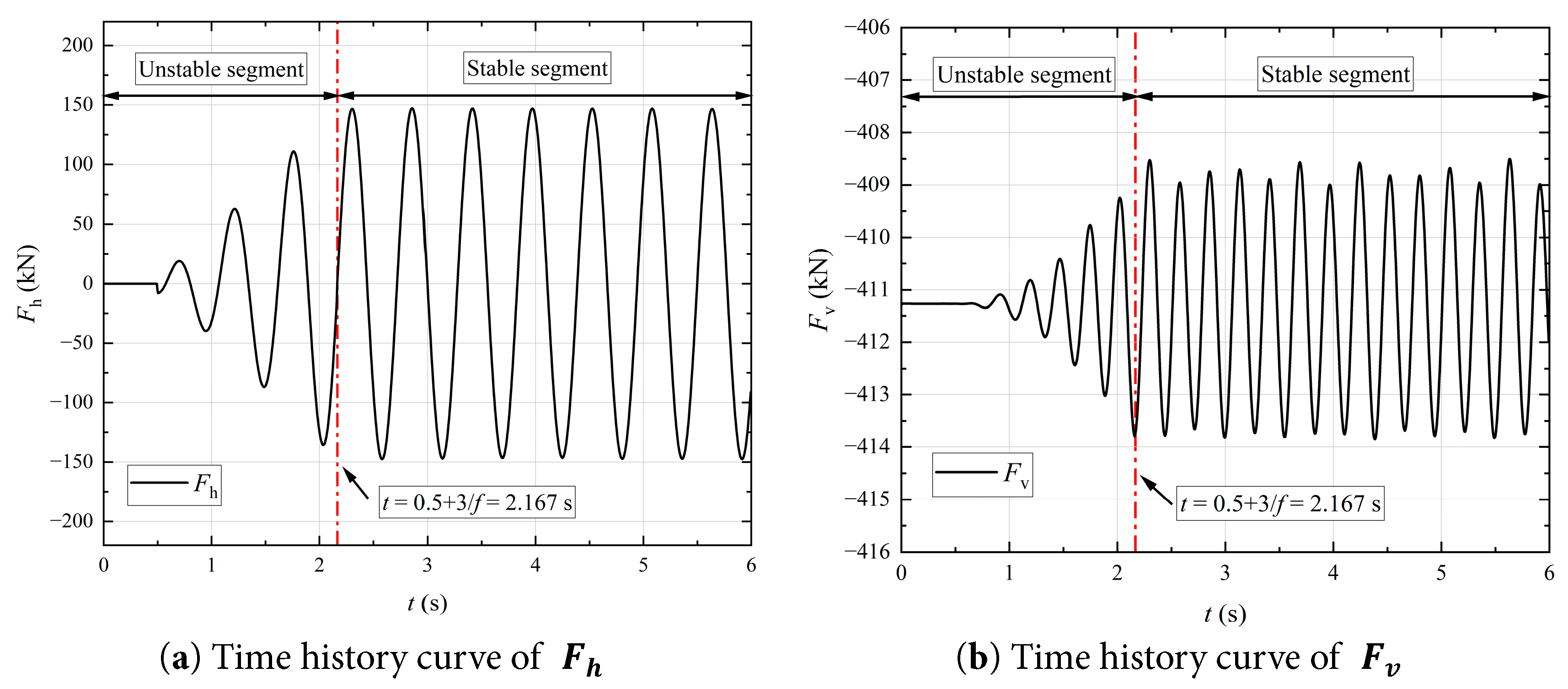
Figure 5: Time history curves of the resultant forces for the Case 0.05–1.8. (a) F h ; (b) F v .

For resonance cases, the motion of the aqueduct continuously transfers energy to the water inside, causing F h and F v to continuously increase. Therefore, the segment from 0.5 + 3 f < t ≤ 7 f + 0.5 is defined as the stable segment of the force time history curves for all the resonance cases manually.

From Fig. 5, regardless of whether the water is in resonance, the frequency of F v curve is twice that of F h curve. To comprehensively demonstrate the dynamic response of the water in the aqueduct under the excitation parameters listed in Table 2, the relationships between the excitation parameters ( A , f ) and the average of maximum values per cycle of the horizontal force, the fluctuating component of the vertical force, and the free surface difference (i.e., F h − m a x a v g , F v f − m a x a v g , Δ h m a x a v g ) in the stable segment are plotted in the subplots of Fig. 6.

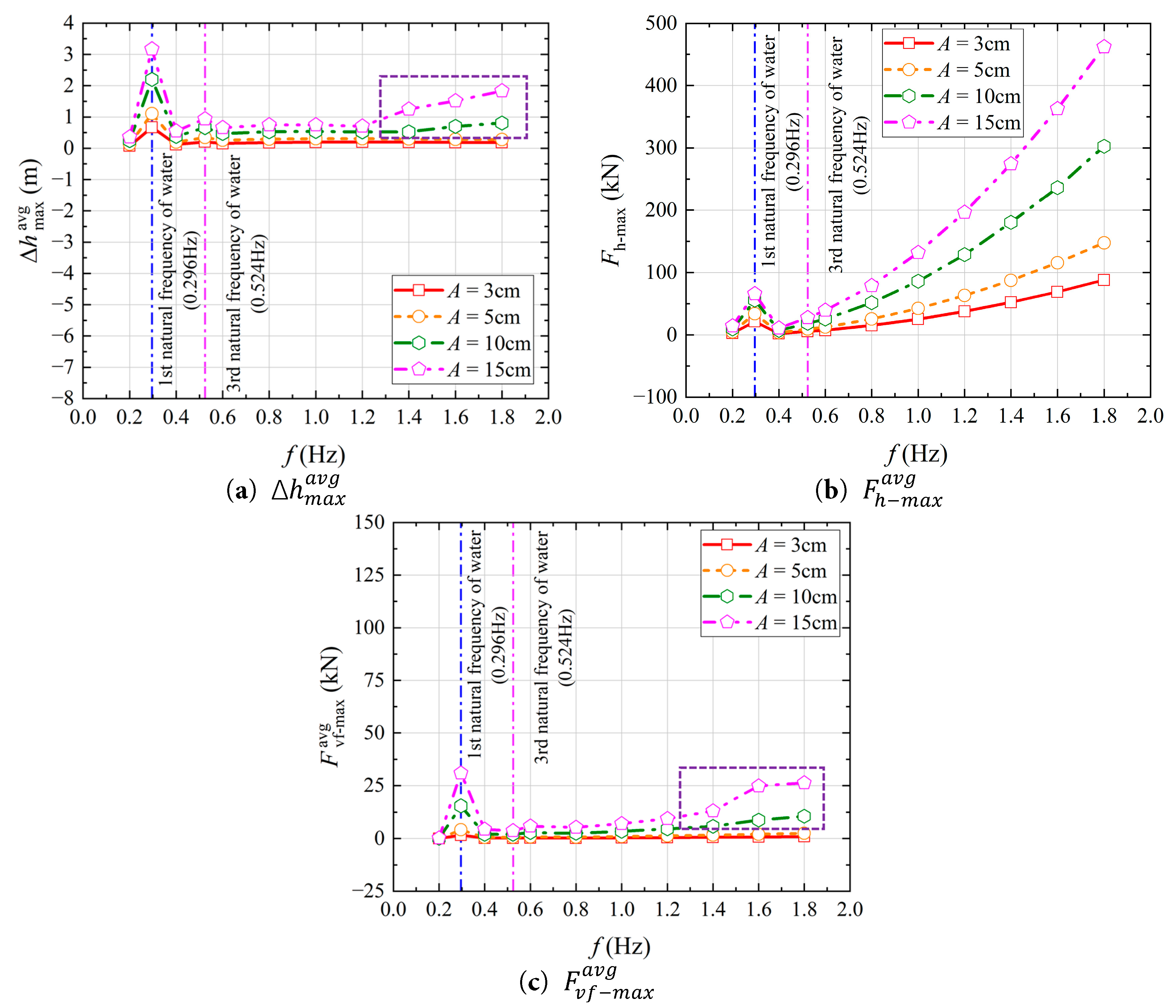
Figure 6: Relationships between the excitation parameters ( A , f ) and the average of maximum values per cycle of the horizontal force, the fluctuating component of the vertical force, and the free surface difference ((a) Δ h m a x a v g , (b) F h − m a x a v g , (c) F v f − m a x a v g , respectively) in the stable segment for all cases in Table 2.

As shown in Fig. 6a, the maximum free surface difference Δ h m a x a v g at the left and right parts of walls exhibits local peaks during both the first-order and third-order resonance of the water. However, for a given A , Δ h m a x a v g during the third-order resonance is only about one-fourth of that during the first-order resonance. Under non-resonance cases, when both the excitation frequency and amplitude are high ( A ≥ 10 cm and f ≥ 1.4 Hz), Δ h m a x a v g generally increases with both f and A , as shown in the purple dashed region in Fig. 6a. Except for the aforementioned cases, Δ h m a x a v g is independent of f and increases only with A .

As shown in Fig. 6b,c, under the first-order resonance cases of water ( f = 0.296 Hz), both F h − m a x a v g , and F v f − m a x a v g exhibit a peak, and this peak increases with A . In regions where the excitation frequency is far from the first-order resonance frequency, the variation of F h − m a x a v g generally follows the trend of the maximum value of the excitation acceleration of the aqueduct a m a x , and F v f − m a x a v g is also independent of f and increases only with A . However, at higher excitation frequencies and amplitudes ( A ≥ 10 cm and f ≥ 1.4 Hz), F v f − m a x a v g increases with both A and f , as shown in the purple dashed region in Fig. 6c. This trend is similar to the variation of Δ h m a x a v g . Moreover, at the excitation frequency f = 0.524 Hz, which corresponds to the third-order natural frequency of the water, F h − m a x a v g and F v f − m a x a v g do not exhibit the pronounced local peak phenomenon observed at the first-order resonance of water.

In summary, the mechanisms behind the generation of the horizontal force F h and vertical force F v can be categorized into the following three cases, which warrant further analysis: (1) First-order resonance of the water ( f = 0.296 Hz ). (2) Non-resonance cases with low excitation frequencies ( 0.4 Hz ≤ f ≤ 1.4 Hz ). (3) Non-resonance cases with high excitation amplitudes and frequencies ( A ≥ 10 cm and f ≥ 1.4 Hz). This study focuses on the generation mechanism of sloshing forces under the first-order resonance cases of the water. To mitigate the influence of transport acceleration induced by the aqueduct’s motion on the water, a resonance case with lower excitation amplitude A (Case 0.05–0.296) is selected for in-depth analysis.

4 Generation Mechanism of Sloshing Forces under Resonance of Water

The time history curves of the normalized horizontal force F ¯ h t , the normalized fluctuating component of the vertical force F ¯ v f t , the normalized displacement d ¯ t , velocity u ¯ t , acceleration a ¯ t , and the normalized free surface difference Δ h ¯ t during one cycle of the stable segment (19.08 s to 22.44 s) for the Case 0.05–0.296, which demonstrates the phase relationships among these normalized physical quantities, are presented in Fig. 7.

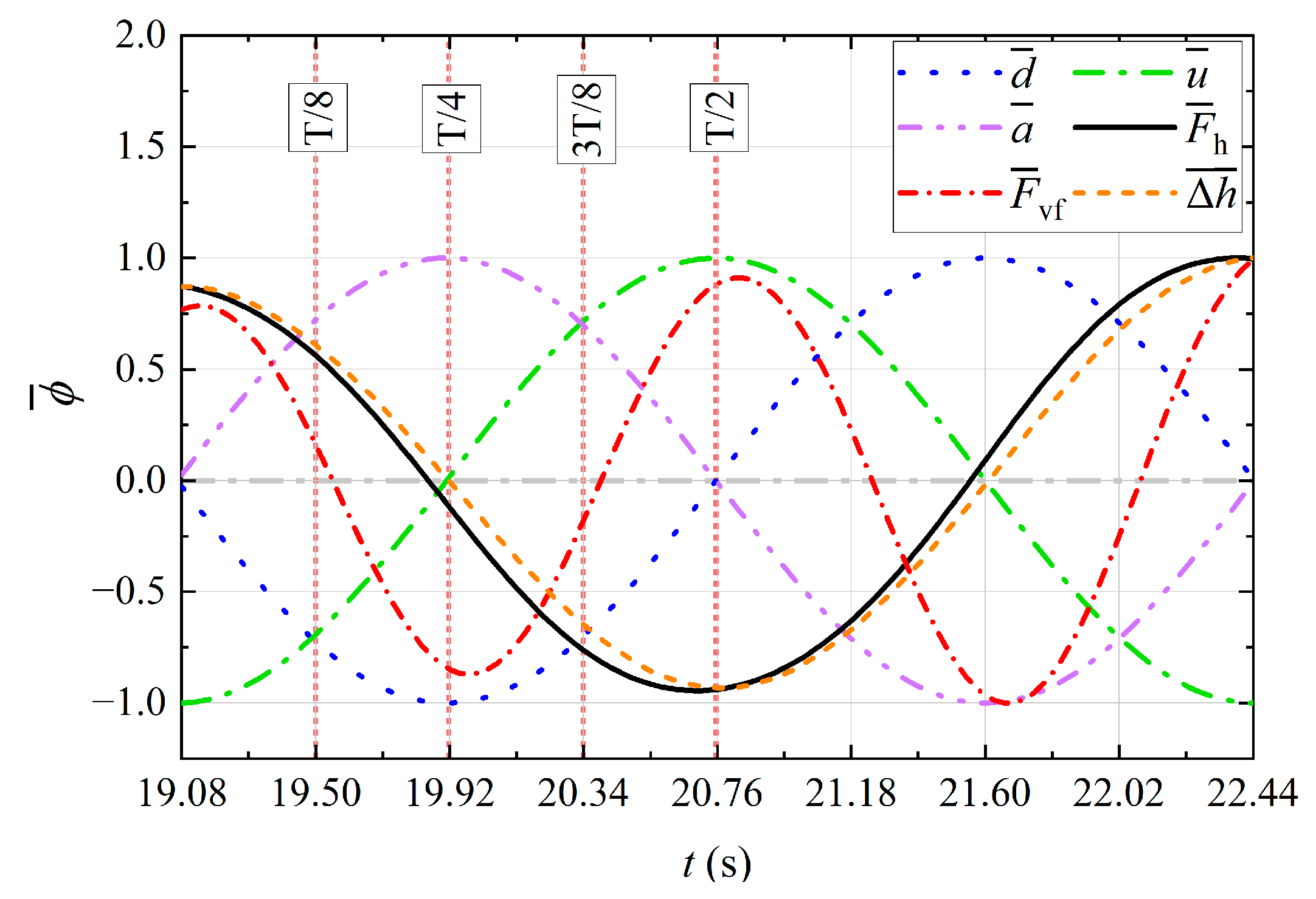
Figure 7: Time history curves of the normalized horizontal force F ¯ h t , the normalized fluctuating component of the vertical force F ¯ v f t , the normalized displacement d ¯ t , velocity u ¯ t , acceleration a ¯ t , and the normalized free surface difference Δ h ¯ t during a cycle in the stable segment (19.08 s to 22.44 s) for the Case 0.05–0.296.

For structural load analysis, the moments when forces reach zero or extreme values are of particular interest. In Fig. 7, additional annotations are provided for the half-cycle ( 0 ∗ T / 8 ~ T / 2 ) during which the aqueduct moves from the equilibrium position ( x = 0 ) to the negative extreme position ( x = − A ) and then back to the equilibrium position, within the time duration t = 19.08 s ~ 22.44 s . The five key moments marked are 0 ∗ T / 8 ( t = 19.08 s ), T / 8 ( t = 19.50 s ) , T / 4 ( t = 19.92 s ), 3 T / 8 ( t = 20.34 s ), and T / 2 ( t = 20.76 s ). The motion in the second half of the cycle (19.08 s to 22.44 s) is identical to the first half, except that the motion direction is reversed.

As shown in Fig. 7, in the Case 0.05–0.296, the F ¯ h t curve essentially coincides with the Δ h ¯ t curve and is nearly the opposite of the u ¯ t curve. The frequency of the F ¯ v f t curve is twice that of the F ¯ h t curve. When d ¯ t is zero, it generally corresponds to the maximum value of F ¯ v f , while when d ¯ t reaches its extreme values, it generally corresponds to the minimum value of F ¯ v f . The peak of the F ¯ v f t curve slightly lags behind the corresponding moments of the d ¯ t curve. The maximum value of the F ¯ h t curve occurs near the 0 moment, the minimum value occurs near the T / 2 moment, and the zero value occurs near the T / 4 moment. The maximum values of the F ¯ v f t curve occur near the 0 and T / 2 moments, the minimum value occurs near the T / 4 moment, and the zero values occur near the T / 8 and 3 T / 8 moments.

F h and F v acting on the aqueduct are essentially derived from the integration of the water pressure distribution over the inner walls. The pressure contours, including dynamic pressure and static pressure, of the water inside the aqueduct at the aforementioned five key moments are shown in Fig. 8 and Fig. 9.

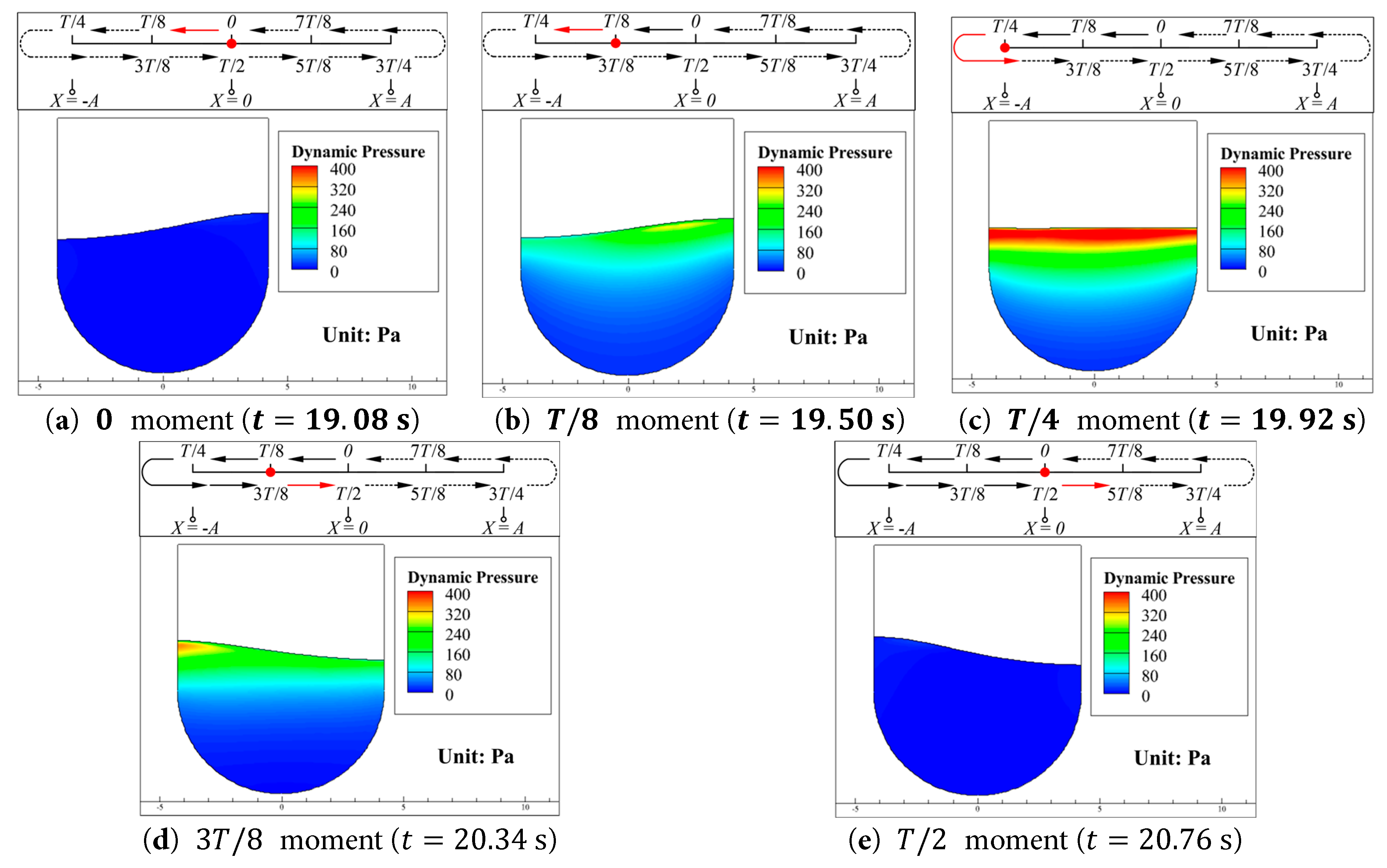
Figure 8: Dynamic pressure contours of the water inside the aqueduct at five key moments during the first half of a cycle in the stable segment (19.08 s to 22.44 s) for the Case 0.05–0.296 (a–e).

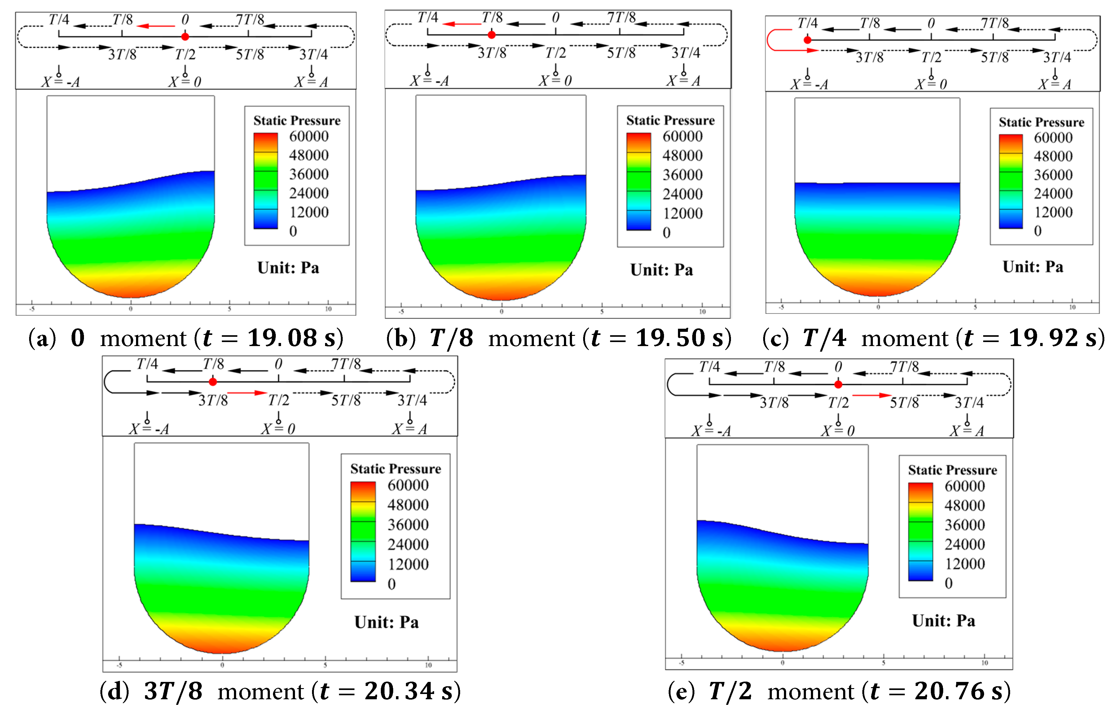
Figure 9: Static pressure contours of the water inside the aqueduct at five key moments during the first half of a cycle in the stable segment (19.08 s to 22.44 s) for the Case 0.05–0.296 (a–e).

As shown in Fig. 8 and Fig. 9, the dynamic pressure is orders of magnitude smaller than the static pressure, and therefore, the dynamic pressure can be neglected in this study. The free surface alternately rises (or falls) at the left and right walls, and the shapes of the free surface is consistent with the experimental observations reported by Li and Wang [34], which confirms that the water inside the aqueduct has undergone first-order resonance.

As shown in Fig. 9a,e, F h reaches its maximum and minimum values at the 0 and T / 2 moments, respectively, and the static pressure contours of the water at these two moments are mirrored in the x-direction. Based on the analysis of Fig. 7, the moments when F h reaches its extreme values generally correspond to the moments when the free surface difference Δ h is at its extreme values. The direction of F h is determined by the sign of Δ h . This means that the mechanisms behind the occurrence of the maximum and minimum values of F h are the same, differing only in the force direction.

F v f reaches its maximum values near the 0 and T/2 moments. This is because, although the pressure field is mirrored horizontally at these two moments, this symmetry has no significant effect on the generation mechanism of F v f in the y-direction. Therefore, when F h changes from its maximum to its minimum value, F v f completes an entire cycle of variation, meaning its frequency is twice that of F h .

In summary, the flow fields (velocity field and pressure field) of the water at the 0 and T / 4 moments are selected for detailed analysis to reveal the generation mechanisms of the extreme and zero values of F h . For the maximum, zero, and minimum values of F v f , the flow fields (velocity field and pressure field) at the 0, T / 8 and T / 4 moments are selected for detailed analysis to reveal their generation mechanisms.

4.1 Analysis of Velocity Filed

The contours of the velocity component u in the x-direction and the velocity component v in the y-direction of the water at the 0, T / 8 , and T / 4 moments are presented in Fig. 10 and Fig. 11, respectively.

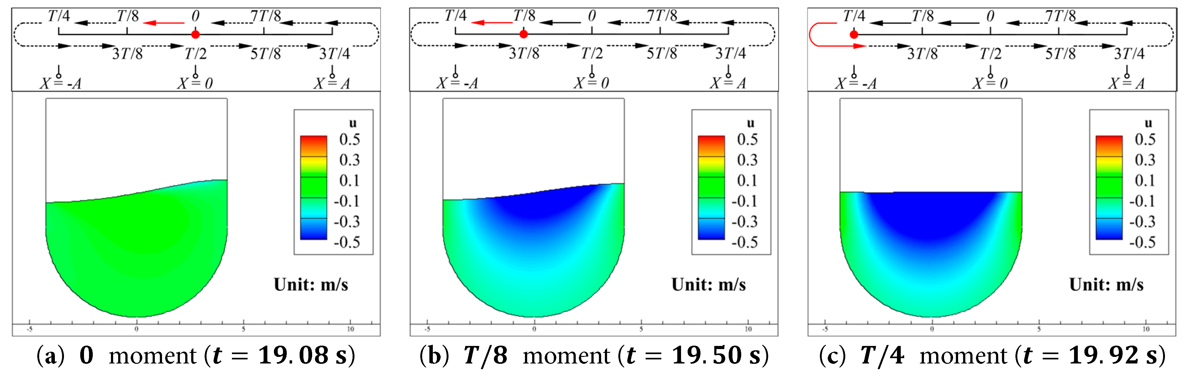
Figure 10: Contours of the velocity component u in the x-direction of the water at the 0, T / 8 , and T / 4 moments during a cycle in the stable segment (19.08 s to 22.44 s) for the Case 0.05–0.296 (a–c).

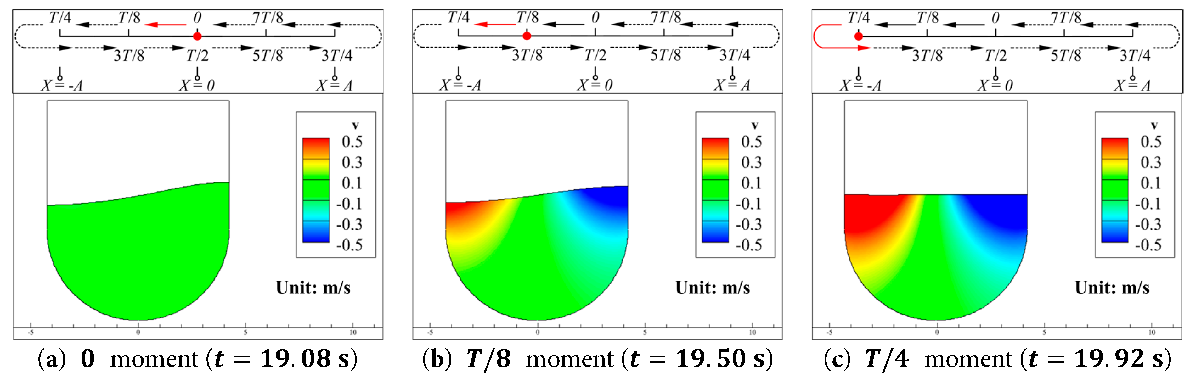
Figure 11: Contours of the velocity component v in the y-direction of the water at the 0, T / 8 , and T / 4 moments during a cycle in the stable segment (19.08 s to 22.44 s) for the Case 0.05–0.296 (a–c).

At the three selected moments, the form of energy in the water inside the aqueduct undergoes significant conversion. Specifically, when Δ h in the aqueduct reaches its maximum (i.e., at the 0 moment, as shown in Fig. 10a and Fig. 11a), the aqueduct moves to the equilibrium position, and the overall velocity of the water is relatively small. The energy of the water is primarily stored as potential energy in the region with higher water level. As shown in Fig. 7, both F h and F v f generated by the water reaches their maximum value at this moment. When the free surface difference in the aqueduct reaches zero (i.e., at the T / 4 moment, as shown in Fig. 10c and Fig. 11c), the aqueduct moves to the maximum horizontal position, and the energy of the water is primarily in the form of kinetic energy. As shown in Fig. 7, F h is nearly zero, and F v f nearly reaches its minimum value at this moment.

The velocity component u in the x-direction of the water is influenced by the wall motion in the near-wall region, especially near the vertical walls. As shown in Fig. 10b,c, the central region of the water exhibits a significant negative u , however, u near the walls is closer to the velocity of wall motion. Comparing Fig. 10a,c, when the energy of the water is primarily in the form of potential energy, u is relatively small. This indicates that the significant negative u in the central region of the water is derived from the conversion of potential energy stored by the water in the region with higher water level. In other words, the free surface fluctuations caused by resonance are the reason for the significant negative u in the central region of the water, rather than the motion of the aqueduct itself. The motion of the aqueduct directly induces the free surface fluctuations, which correspond to the velocity component v in the y-direction of the water. Since the free surface fluctuations decrease gradually from the vertical walls to the center of the aqueduct, the velocity component v in the y-direction follows the same pattern, as shown in Fig. 11b,c. Additionally, regions with higher absolute value of v are concentrated near the free surface, which means the magnitude of v decreases with increasing depth.

4.2 Analysis of Static Pressure Variation ΔP_s

To investigate the generation mechanisms of F h and F v f acting on the aqueduct in detail, the static pressure of the water in the stationary state ( P 0 ) is subtracted from the static pressure of the water at each moment during the aqueduct’s motion ( P ) calculated by the CFD model to obtain the static pressure variation Δ P s , as shown in Eq. (6). By integrating Δ P s over the no-slip walls, F h and F v f can be determined.

In this study, for the convenience of analyzing the contours of various physical quantities in the flow field, the following annotations are made on each contours: the red dash line indicates the free surface at a moment, the blue dash dot line represents the free surface in the stationary state, the green double dot dash line indicates the boundary between the rectangular and semicircular parts of the U-shaped aqueduct, the purple dot line represents the symmetry axis of the aqueduct, the orange solid line denotes the contour where Δ P s = 0 inside the water, and the orange hollow dots mark the points where the free surface fluctuation is zero.

The contours of the static pressure variation Δ P s of the water inside the aqueduct at the 0, T / 8 , and T / 4 moments are shown in Fig. 12.

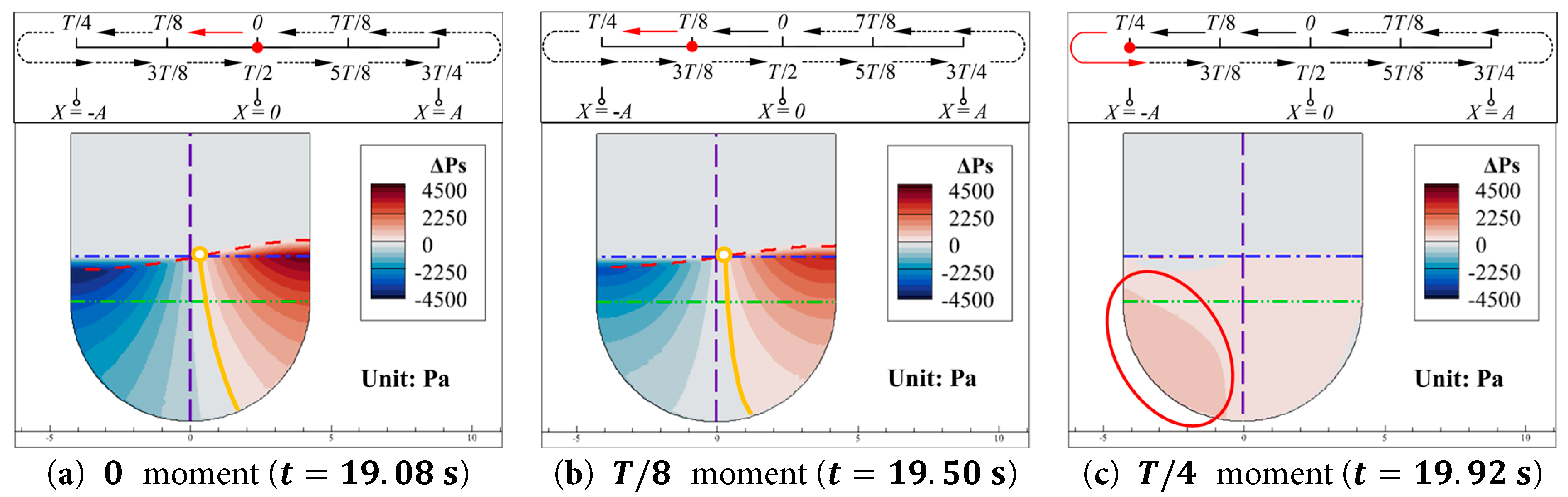
Figure 12: Contours of the static pressure variation Δ P s of the water inside the aqueduct at the 0, T / 8 , and T / 4 moments during a cycle in the stable segment (19.08 s to 22.44 s) for the Case 0.05–0.296 (a–c).

From Fig. 12, it can be observed that as the free surface alternately rises (or falls) at the left and right walls, the static pressure variation Δ P s of the water is also broadly divided into regions with positive and negative values. When there is a free surface difference in the aqueduct, as shown in Fig. 12a,b, Δ P s > 0 in regions where the free surface rises, while Δ P s < 0 in regions where the free surface falls. This indicates that changes in the height of free surface are one of the reasons for the variation in static pressure of the water.

Regions with higher absolute values of Δ P s are concentrated near the free surface close to the left and right walls. At a given depth, the absolute value of Δ P s gradually decreases from the near-wall regions toward the center of the aqueduct. This is because, during the first-order resonance of the water, the amplitude of the free surface fluctuations decreases from the walls to the center of the aqueduct. However, the contour line where Δ P s = 0 (indicated by the orange solid line) does not coincide with the symmetry axis of the aqueduct, as shown in Fig. 12a,b. Instead, it shifts toward the region where Δ P s > 0 . In Fig. 12a,b, the orange hollow dots represent the intersection points of the Δ P s = 0 contour, the current free surface shape, and the free surface shape in the stationary state, i.e., the points where the free surface fluctuation is zero at that moment. By observing the positions of these zero-fluctuation points at the 0 and T / 8 moments in Fig. 12, it is found that when there is a free surface difference between the left and right walls, the zero-fluctuation points also shift toward the region where Δ P s > 0 . Additionally, the free surface falls slightly at the symmetry axis of the aqueduct, indicating that the region where the free surface rises is smaller than the region where it falls. The height of the water rising at one wall is always greater than the height of the water falling at the opposite wall at the same moment. This suggests that the alternating rise (or fall) of the free surface at the left and right walls during the first-order resonance of the water is not symmetric, and the free surface fluctuations are not purely standing waves. As shown in Fig. 10, during the period from 0 to T / 4 , the aqueduct moves from the equilibrium position to the maximum horizontal position. In this process, the central region of the water exhibits a negative horizontal (x-direction) velocity component u . This indicates that a portion of the surface water undergoes horizontal flow, leading to the aforementioned asymmetry in free surface fluctuations. This asymmetry in free surface fluctuations also causes the contour line where Δ P s = 0 (indicated by the orange solid line) to consistently shift toward the region where Δ P s > 0 .

As shown in Fig. 12a,b, the region enclosed by the red dash line and the blue dash dot line can be divided into two areas based on the sign of Δ P s : the region where Δ P s > 0 (referred to as the water increase zone) and the region where Δ P s < 0 (referred to as the water decrease zone). In these two types of regions, compared to the stationary state of the water, the rise (or fall) of the free surface causes areas that were originally free of water to now be occupied by water (water increase zone) or areas that originally contained water to now be free of water (water decrease zone). Therefore, when calculating Δ P s by Eq. (6), in addition to the change in free surface height, the change in fluid density compared to the stationary state is also considered. This results in the absolute value of Δ P s in these regions increasing with depth until reaching a maximum value on the walls. When there is no free surface difference in the aqueduct, as shown in Fig. 12c, the Δ P s of the water in the aqueduct is mostly greater than or equal to zero. Except for a region with higher Δ P s near the bottom of the left half of the aqueduct (indicated by the red circle in Fig. 12c), the Δ P s in most regions of the water is close to zero.

4.3 Influence of Acceleration Field

Studies by many scholars (e.g., Refs. [35,36]) have shown that the viscosity of the liquid can be neglected in the analysis of liquid sloshing phenomena in containers. And Ref. [29] also shows that fluid viscosity only affects the amplitude of the surface oscillation without altering the temporal profile; hence, the Euler equations are employed herein to elucidate the underlying mechanism of sloshing-induced loads.

The Euler equations in the horizontal (x-direction) and vertical (y-direction) directions are given as follows: ∂ux,y,t∂t+ux,y,t∂ux,y,t∂x+vx,y,t∂ux,y,t∂y=−1ρx,y,t∂Px,y,t∂x,(7) ∂vx,y,t∂t+ux,y,t∂vx,y,t∂x+vx,y,t∂vx,y,t∂y=g−1ρx,y,t∂Px,y,t∂y,(8) where u x , y , t , v x , y , t represent the velocity components in the x and y directions, respectively; P x , y , t is the static pressure field of the fluid; ρ x , y , t is the density of the two-phase flow in the container.

Since the Euler equations essentially represent Newton’s second law in fluid mechanics, the left-hand side of the Euler equations describes the acceleration generated by the fluid velocity field. Specifically, the left-hand side of Eq. (7) is the material derivative of u x , y , t , where ∂ u x , y , t ∂ t is the local acceleration of u , and u x , y , t ∂ u x , y , t ∂ x + v x , y , t ∂ u x , y , t ∂ y is the convective acceleration of u . Similarly, the left-hand side of Eq. (8) is the material derivative of v x , y , t , where ∂ v x , y , t ∂ t is the local acceleration of v , and u x , y , t ∂ v x , y , t ∂ x + v x , y , t ∂ v x , y , t ∂ y is the convective acceleration of v .

Based on the analysis of the spatial distribution of Δ P s , it is evident that the free surface fluctuations cause changes in Δ P s . If only the influence of free surface fluctuations is considered, Δ P s should remain constant along the depth direction (y-direction) in the region outside the water increase zone and the water decrease zone (referred to as the constant density zone). However, in this region, the absolute value of Δ P s gradually decreases with increasing depth. Therefore, considering the Euler equations in two dimensions as shown in Eqs. (7) and (8), the additional acceleration generated by the velocity field in the vertical direction consists of two parts: the local acceleration of v , ∂ v ∂ t , and the convective acceleration of v , u ∂ v ∂ x + v ∂ v ∂ y . Similarly, the additional acceleration generated by the velocity field in the horizontal direction also consists of the local acceleration of u , ∂ u ∂ t , and the convective acceleration of u , ∂ u ∂ x + v ∂ u ∂ y . The following treatment is applied to the Euler equation in the y-direction (Eq. (8)):

In the stationary state, the velocity of the water is zero. Therefore, substituting u = v = 0 into Eq. (8), we obtain: 0=g−1ρ0∂P0∂y,(9) during the motion of the aqueduct, substituting Eq. (9) into Eq. (8), we obtain: ∂vx,y,t∂t+ux,y,t∂vx,y,t∂x+vx,y,t∂vx,y,t∂y=1ρ0x,y∂P0x,y∂y−1ρx,y,t∂Px,y,t∂y,(10) where u x , y , t , v x , y , t are the velocity fields in the x-direction and y-direction, respectively, at time t during the motion of the aqueduct; P 0 x , y is the static pressure field of the fluid in the stationary state of the aqueduct; P x , y , t is the static pressure field of the fluid at time t ; ρ 0 x , y is the density field of the fluid in the stationary state of the aqueduct; and ρ x , y , t is the density field of the fluid at time t . Except for the water increase zone and the water decrease zone in Fig. 12, the remaining regions do not involve changes in the density of the fluid occupying these regions. Therefore, it can be assumed that in these regions, x , y , t = ρ 0 x , y = ρ w a t e r . Thus, Eq. (10) can be further simplified as: ∂vx,y,t∂t+ux,y,t∂vx,y,t∂x+vx,y,t∂vx,y,t∂y=−1ρwater∂ΔPsx,y,t∂y,(11) from Eq. (11), it can be seen that changes in the velocity field affect the gradient of Δ P s along the y-direction. When the sum of the local acceleration and convective acceleration on the left side of Eq. (11) is positive, ∂ Δ P s x , y , t ∂ y is negative, meaning that Δ P s increases with increasing depth (y decreasing). Conversely, when the sum of the local acceleration and convective acceleration is negative, ∂ Δ P s x , y , t ∂ y is positive, meaning that Δ P s decreases with increasing depth (y decreasing). When calculating Δ P s in the water increase zone, the influence of the vertical local acceleration and convective acceleration has already been considered in the gravitational acceleration. In the water decrease zone, Δ P s decreases linearly with depth increasing according to the static pressure calculation method ( p = ρ g h ) until reaching the extreme value position at that moment.

The contours of the local acceleration in the y-direction ∂ v ∂ t of the water inside the aqueduct at the 0, T / 8 , and T / 4 moments are shown in Fig. 13.

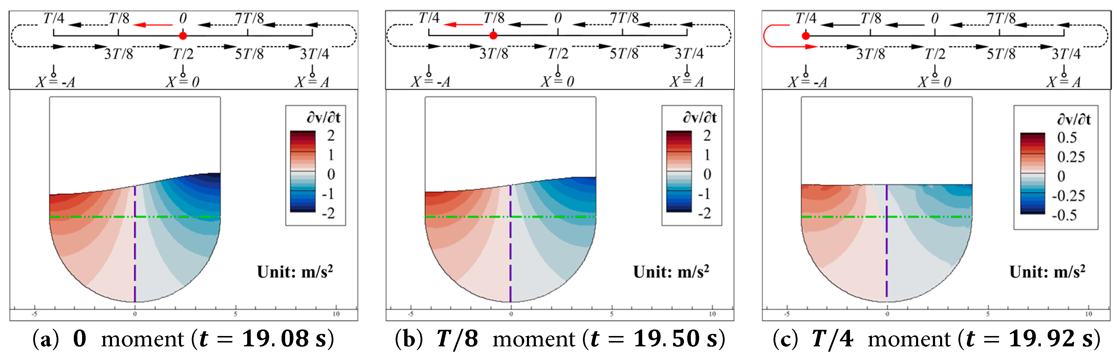
Figure 13: Contours of the local acceleration in the y-direction ∂ v ∂ t of the water inside the aqueduct at the 0, T / 8 , and T / 4 moments during a cycle in the stable segment (19.08 s to 22.44 s) for the Case 0.05–0.296 (a–c).

The contours of the convective acceleration in the y-direction u ∂ v ∂ x + v ∂ v ∂ y of the water inside the aqueduct at the 0, T / 8 , and T / 4 moments are shown in Fig. 14.

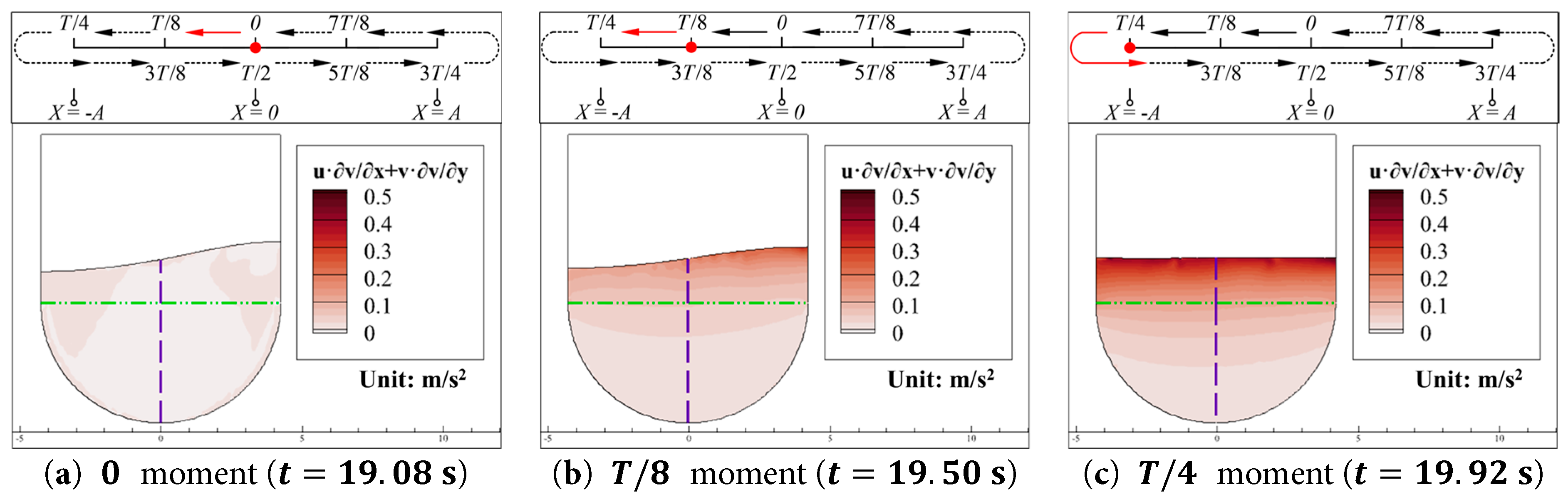
Figure 14: Contours of the convective acceleration in the y-direction u ∂ v ∂ x + v ∂ v ∂ y of the water inside the aqueduct at the 0, T / 8 , and T / 4 moments during a cycle in the stable segment (19.08 s to 22.44 s) for the Case 0.05–0.296 (a–c).

As shown in Fig. 13, since the direction of free surface fluctuations is opposite at the left and right walls, the sign of the local acceleration in the vertical direction ∂ v ∂ t is also opposite at the left and right walls. The regions with positive and negative values of ∂ v ∂ t are mostly distributed on either side of the symmetry axis of the aqueduct. Consistent with the distribution pattern of the vertical velocity component v shown in Fig. 11, the absolute value of ∂ v ∂ t is larger near the vertical walls and the free surface, while it is smaller in the central region of the aqueduct, and the absolute value of ∂ v ∂ t gradually decreases with increasing depth. From Fig. 13, it can also be observed that in the semicircular part of the fluid domain (below the green double dot dash line), the distribution of the absolute value of ∂ v ∂ t is essentially symmetric. That is, the differences in the absolute value of ∂ v ∂ t about the symmetry axis are mainly concentrated near the vertical walls and the free surface. Due to the fact that during resonance, the rise of the water at one wall is greater than its fall at the opposite wall, the absolute value of ∂ v ∂ t in the water increase zone is larger than that in the water decrease zone, as shown in Fig. 13a,b. Additionally, it can be observed that when the free surface is higher than its stationary state, ∂ v ∂ t in the corresponding region is negative. Conversely, when the free surface is lower than its stationary state, ∂ v ∂ t in the corresponding region is positive. This is because, during the motion of the aqueduct, when the free surface deviates from its stationary position, gravity, as the only restoring force in the vertical direction, always tends to restore the free surface to its stationary position, resulting in the direction of ∂ v ∂ t being opposite to the free surface fluctuations. When Δ h in the aqueduct is small, as shown in Fig. 13c, the free surface fluctuation velocity reaches its extreme value, leading to a significant reduction in the absolute value of the vertical local acceleration ∂ v ∂ t .

The convective acceleration in the vertical direction u ∂ v ∂ x + v ∂ v ∂ y remains positive during the motion of the aqueduct and gradually decreases with increasing depth, as shown in Fig. 14. This is because, from a physical perspective, u ∂ v ∂ x + v ∂ v ∂ y represents the acceleration in the vertical direction caused by changes in the geometric shape of the region occupied by the water inside the aqueduct. In this case, the region where the geometric shape of the water changes most dramatically is near the free surface. When Δ h is nearly at its maximum, as shown in Fig. 14a, the energy of the water is primarily in the form of potential energy, and the free surface fluctuations are slow, meaning the geometric shape of the water changes slowly. Therefore, u ∂ v ∂ x + v ∂ v ∂ y is not significant. When the energy of the water is primarily in the form of kinetic energy, Δ h is small, and the free surface fluctuations are more intense. As a result, the geometric shape of the water changes more dramatically, and u ∂ v ∂ x + v ∂ v ∂ y is higher, as shown in Fig. 14c. When the energy of the water is in the process of converting between potential and kinetic energy, as shown in Fig. 14b, due to the asymmetry of the free surface fluctuations, the rise of the water at one wall is greater than its fall at the opposite wall at the same moment. Therefore, the water above the stationary free surface has a higher velocity, meaning the geometric shape changes more dramatically in the water increase zone. Consequently, u ∂ v ∂ x + v ∂ v ∂ y in the water increase zone is higher compared to other regions of the water.

By combining the analysis of Fig. 13 and Fig. 14, it can be observed that when the energy of the water inside the aqueduct is primarily in the form of potential energy, the free surface height changes slowly, and Δ h in the aqueduct is significant. In this case, u ∂ v ∂ x + v ∂ v ∂ y can be neglected, as shown in Fig. 14a. However, at this time, the water exhibits significant vertical local acceleration ∂ v ∂ t , as shown in Fig. 13a. On the other hand, when the energy of the water is primarily in the form of kinetic energy, the free surface difference in the aqueduct is negligible, and the free surface fluctuation velocity reaches its maximum. As a result, the absolute value of ∂ v ∂ t decreases significantly, as shown in Fig. 13c, while u ∂ v ∂ x + v ∂ v ∂ y becomes prominent, as shown in Fig. 14c. In other words, as the energy of the water converts from potential to kinetic energy, the absolute value of ∂ v ∂ t gradually decreases, while u ∂ v ∂ x + v ∂ v ∂ y gradually increases, and vice versa.

From Eq. (7), it can be seen that ∂ P x , y , t ∂ x is influenced by the acceleration terms on the left side of the equation, where ∂ u x , y , t ∂ t is the local acceleration of u , and u x , y , t ∂ u x , y , t ∂ x + v x , y , t ∂ u x , y , t ∂ y is the convective acceleration of u . This means that during the motion of the aqueduct, the horizontal acceleration of the water also affects the gradient of the static pressure in the horizontal direction.

The contours of the local acceleration in the x-direction ∂ u ∂ t of the water inside the aqueduct at the 0, T / 8 , and T / 4 moments are shown in Fig. 15.

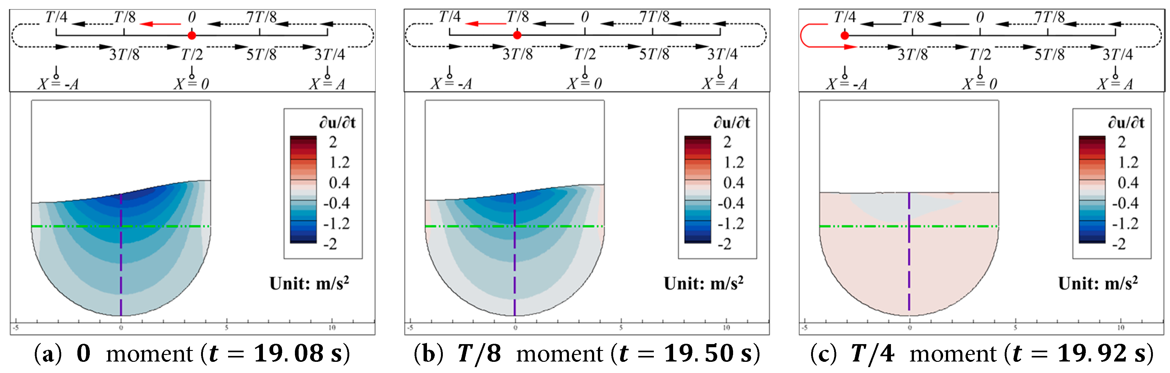
Figure 15: Contours of the local acceleration in the x-direction ∂ u ∂ t of the water inside the aqueduct at the 0, T / 8 , and T / 4 moments during a cycle in the stable segment (19.08 s to 22.44 s) for the Case 0.05–0.296 (a–c).

The contours of the convective acceleration in the x-direction u ∂ u ∂ x + v ∂ u ∂ y of the water inside the aqueduct at the 0, T / 8 , and T / 4 moments are shown in Fig. 16.

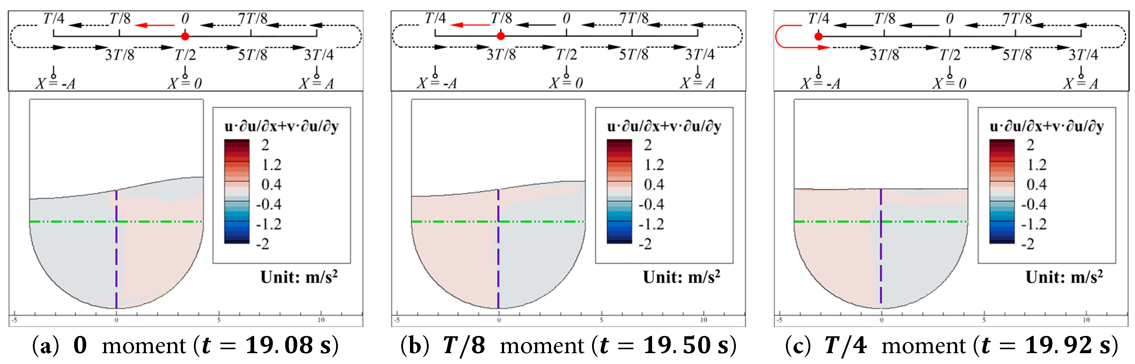
Figure 16: Contours of the convective acceleration in the x-direction u ∂ u ∂ x + v ∂ u ∂ y of the water inside the aqueduct at the 0, T / 8 , and T / 4 moments during a cycle in the stable segment (19.08 s to 22.44 s) for the Case 0.05–0.296 (a–c).

As shown in Fig. 16, since first-order resonance occurs in the Case 0.05–0.296, the free surface primarily fluctuates in the y-direction, and thus u ∂ u ∂ x + v ∂ u ∂ y can be neglected. The absolute value of ∂ u ∂ t reaches its maximum value at the 0 moment ( t = 19.08 s ), as shown in Fig. 15a. This is because, at this moment, the energy of the water is at the critical point of converting from potential to kinetic energy, and the velocity of the water is almost zero, as shown in Fig. 10a and Fig. 11a. As the free surface difference gradually decreases, ∂ u ∂ t reaches zero at the T / 4 moment ( t = 19.92 s ), as shown in Fig. 15c. At this time, the energy of the water is almost entirely in the form of kinetic energy, and the horizontal velocity u reaches its maximum, as shown in Fig. 10c. Therefore, the local horizontal acceleration ∂ u ∂ t is almost zero at this moment.

Combining Fig. 15 and Fig. 16, it can be observed that the non-zero regions of ∂ u ∂ t are mainly concentrated near the free surface in the central region of the water. That is, at the same depth, the absolute value of ∂ u ∂ t is smaller near the walls and larger in the central region of the water. In the depth direction (y-direction), the absolute value of ∂ u ∂ t also gradually decreases. This suggests that, in the Case 0.05–0.296, ∂ u ∂ t is caused by the vertical fluctuations of the free surface and the conversion between potential and kinetic energy of the water inside the aqueduct. As discussed in the analysis of Fig. 12, during the resonance of the water, the surface water also undergoes some degree of horizontal flow, which manifests as ∂ u ∂ t .

In summary, the free surface fluctuations caused by resonance are the reason for the horizontal local acceleration ∂ u ∂ t in the central region of the water, rather than the motion of the aqueduct itself. This conclusion is consistent with the analysis of the velocity field of the water in Section 4.1. Based on the above analysis based on the Euler equations, the static pressure variation Δ P s of the water inside the aqueduct in the Case 0.05–0.296 is primarily influenced by the local acceleration ∂ v ∂ t and the convective acceleration u ∂ v ∂ x + v ∂ v ∂ y in the vertical direction.

4.4 Generation Mechanism of Horizontal Force F_h

The forces exerted on the aqueduct by the water (including the horizontal force F h and the fluctuating component of the vertical force F v f ) originate from changes in the static pressure of the water during the sloshing process. The moments when F h reaches its extreme and zero values are selected as the research focus. The distribution of Δ P s along the height direction (y-direction) on the left and right walls of the aqueducts at the 0 and T / 4 moments for the Case 0.05–0.296 are shown in Fig. 17. The blue dash dot line represents the free surface in the stationary state y = 1.61 , the green double dot dash line indicates the boundary between the rectangular and semicircular parts of the U-shaped aqueduct, red circle marks the position where the extreme value of Δ P s occurs on the left wall, black diamond marks the position where the extreme value of Δ P s occurs on the right wall, red triangle indicates the position where the y-coordinate is 0 on the left wall, black square indicates the position where the y-coordinate is 0 on the right wall, and purple star represents the lowest point of the aqueduct.

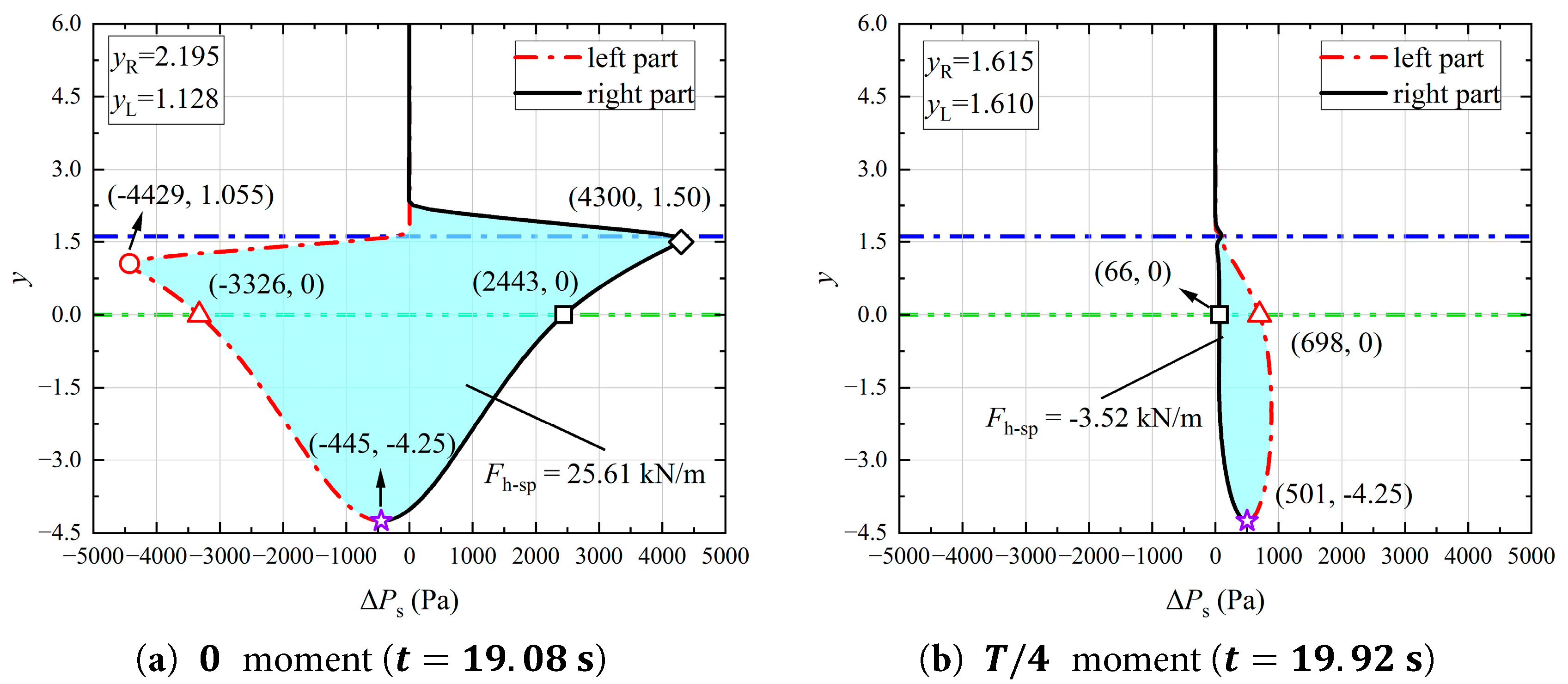
Figure 17: Distribution of Δ P s along the height direction (y-direction) on the left and right walls of the aqueducts at the 0 and T / 4 moments during a cycle in the stable segment (19.08 s to 22.44 s) for the Case 0.05–0.296 (a,b).

At the 0 moment ( t = 19.08 s ), the water inside the aqueduct falls at the left wall and rises at the right wall. The extreme point of Δ P s on the left wall, marked by red circle, has coordinates (−4429, 1.055), slightly below the free surface at the left wall y L = 1.128 at this moment, as shown in Fig. 17a. This is because the Volume of Fluid (VOF) method is used in this study to capture the free surface. In the VOF method, the volume fraction α of the water near the interface between the two phases is a continuously varying quantity from 0 to 1. In this study, the free surface position corresponds to the location where the volume fraction α is 0.5. Therefore, at y L = 1.128 , the fluid density is the average of the densities of water and air, which is lower than the density of water. This means that the influence of fluid density at the free surface is still significant. Consequently, when calculating Δ P s by Eq. (6), the extreme value of Δ P s does not occur at y L = 1.128 . As the depth increases, α gradually changes from 0.5 to 1, and the fluid density increases from the average of the densities of water and air to the density of water ( ρ w a t e r = 998.2 kg / m 3 ). The influence of fluid density on Δ P s gradually weakens, allowing Δ P s to reach its extreme value. Similarly, the water inside the container rises at the right wall. The extreme point of Δ P s on the right wall, marked by black diamond, has coordinates (4300, 1.5), as shown in Fig. 17a. The asynchrony between the free surface and the influence of fluid density on Δ P s , caused by the VOF method, results in the extreme value of Δ P s on the right wall being slightly below the free surface in the stationary state y R = 1.61 .

The free surface fluctuation at the right wall is 21.9% higher than that at the left wall, but the absolute value of the extreme Δ P s on the right wall is 2.9% lower than that on the left wall. As shown in Fig. 13a, the rise of the water at the right wall results in a negative vertical local acceleration ∂ v ∂ t in this region, while the fall of the water at the left wall results in a positive ∂ v ∂ t in that region. As pointed out in the analysis of Fig. 12, free surface fluctuations are a significant factor in the generation of Δ P s . When the free surface rises in a certain region, Δ P s in that region also increases, and vice versa. Additionally, based on the analysis of Eqs. (15) and (16), a negative ∂ v ∂ t causes Δ P s to decrease with increasing depth, while a positive ∂ v ∂ t causes Δ P s to increase with increasing depth. Therefore, ∂ v ∂ t and free surface fluctuations have opposite effects on Δ P s . When calculating Δ P s at the right wall, since the gravitational acceleration in the water increase zone already accounts for the influence of the negative ∂ v ∂ t , the negative ∂ v ∂ t reduces the extreme value of Δ P s on the right wall to some extent, despite the larger free surface fluctuation at the right wall. Furthermore, in the constant density zone of the rectangular part of the aqueduct, the influence of ∂ v ∂ t causes the absolute value of Δ P s distribution on the left and right walls to decrease with increasing depth. On the other hand, in the semicircular part of the container, as the depth increases, the walls become closer to the central region of the aqueduct. Therefore, the influence of both free surface fluctuations and ∂ v ∂ t on Δ P s weakens, leading to a rapid decrease in the absolute value of Δ P s distribution with increasing depth in this region.

When Δ h = 0 , the energy of the water is primarily in the form of kinetic energy, and the influence of the convective acceleration u ∂ v ∂ x + v ∂ v ∂ y cannot be neglected. Taking Fig. 17b as an example, at the T / 4 moment ( t = 19.92 s), both ∂ v ∂ t and u ∂ v ∂ x + v ∂ v ∂ y must be considered. As shown in Fig. 13c, ∂ v ∂ t is positive at the left wall and negative at the right wall, with higher absolute values concentrated near the free surface and the walls. As shown in Fig. 14c, u ∂ v ∂ x + v ∂ v ∂ y is higher near the free surface and decreases with increasing depth, with little variation along the horizontal direction. Therefore, when both ∂ v ∂ t and u ∂ v ∂ x + v ∂ v ∂ y are considered, the superposition of these two accelerations results in a higher positive acceleration near the free surface and the left wall, causing Δ P s in this region to increase. On the other hand, in the right half of the aqueduct, ∂ v ∂ t and u ∂ v ∂ x + v ∂ v ∂ y cancel each other out, resulting in Δ P s being close to zero in this region, as shown in Fig. 17c. Similarly, this also explains the phenomenon observed in Fig. 12c, where “Except for a region with higher Δ P s near the bottom of the left half of the aqueduct (indicated by the red circle in Fig. 12c), the Δ P s in most regions of the water is close to zero.”

4.5 Generation Mechanism of Fluctuating Component of Vertical Force F_vf

The vertical force F v acts only on the semicircular walls of the U-shaped aqueduct. The moments when the fluctuating component of the vertical force F v f reaches its extreme and zero values are selected as the research focus. The distribution of Δ P s along the horizontal direction (x-direction) on this part at the 0, T / 8 and T / 4 moments for the Case 0.05–0.296 are shown in Fig. 18.

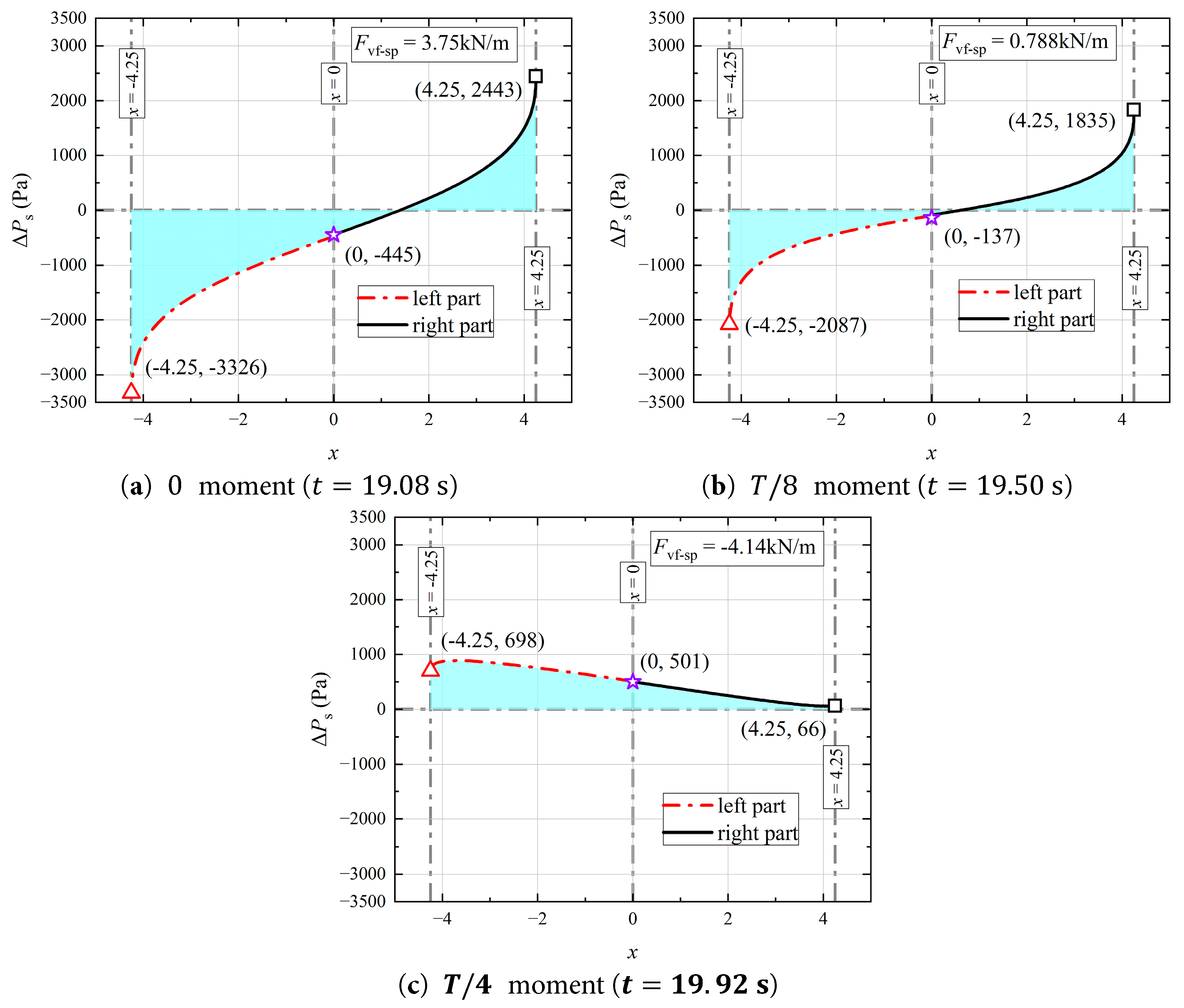
Figure 18: Distribution of Δ P s along the horizontal direction (x-direction) on the semicircular walls of the aqueduct at the 0, T / 8 and T / 4 moments during a cycle in the stable segment (19.08 s to 22.44 s) for the Case 0.05–0.296 (a–c).

Regarding the change in Δ P s at the lowest point of the aqueduct during its motion, as shown in Fig. 13, the vertical local acceleration ∂ v ∂ t is essentially zero on the symmetry axis of the aqueduct and can be neglected.

When the energy of the water is in the form of potential energy, as shown in Fig. 17a, the fall in the free surface at the symmetry axis due to the asymmetry of free surface fluctuations is the main reason for the decrease in Δ P s at the lowest point of the aqueduct. At this moment, the Δ P s at the position marked by purple star is −445 Pa, as shown in Fig. 17a and Fig. 18a. Since the positions marked by red star and black square are located at the tangent points between the semicircular walls and the vertical walls of the aqueduct, the Δ P s at these positions is influenced by both the free surface fluctuations and the vertical local acceleration ∂ v ∂ t . As shown in Fig. 18a, the absolute value of Δ P s at the position marked by red tringle on the left part of the semicircle walls is 36.14% higher than that at the same position on the right part, marked by black square. However, comparing this with Fig. 17a, the absolute value of the extreme Δ P s on the left wall is 2.9% higher than that on the right wall. From Fig. 13a, it can be seen that in the constant density zone, the absolute value of ∂ v ∂ t is symmetrically distributed along the symmetry axis. Therefore, the average slope of the Δ P s distribution curve between points marked by black diamond and square on the left wall is not significantly different from that between points marked by red circle and tringle on the right wall, as shown in Fig. 17a. However, due to the fall of the free surface at the left wall, the difference in the y-coordinates between points marked by red circle and tringle is 1.055, while due to the rise of the free surface at the right wall, the difference in the y-coordinates between points marked by black diamond and square is 1.50. This results in ∂ v ∂ t having a different influence height on the reduction of the absolute value of Δ P s on the left and right vertical walls. Since the difference in the y-coordinates between points marked by red circle and tringle is 29.67% smaller than that between points marked by black diamond and square, the reduction in the absolute value of Δ P s at the point marked by red tringle on the left wall is smaller than that at the point marked by black square on the right wall, i.e., the absolute value of Δ P s at the point marked by red tringle on the left wall is higher than that at the point marked by black square on the right wall. In summary, as shown in Fig. 18a, at the 0 moment ( t = 19.08 s ), the area of the negative Δ P s region on the semicircular wall is larger than that of the positive Δ P s region, leading to the occurrence of the maximum value of F v f .

When the energy of the water inside the aqueduct converts from potential to kinetic energy, as shown in Fig. 14b, the free surface position at the symmetry axis rises slightly as Δ h decreases, and the vertical convective acceleration u ∂ v ∂ x + v ∂ v ∂ y gradually increases. Under the combined influence of these two factors, the Δ P s (−137 Pa) at the lowest point of the aqueduct (marked by purple star in Fig. 18b) increases. On the other hand, the decrease in Δ h in the aqueduct leads to a reduction in the absolute values of the extreme Δ P s on both the left and right walls, as well as a decrease in the absolute value of the vertical local acceleration ∂ v ∂ t (as shown in Fig. 13b). When both ∂ v ∂ t and u ∂ v ∂ x + v ∂ v ∂ y are considered, as shown in Fig. 13b and Fig. 14b, it is found that u ∂ v ∂ x + v ∂ v ∂ y balances, to some extent, the phenomenon where the absolute value of ∂ v ∂ t in the water increase zone is larger than that in the water decrease zone due to the asymmetry of free surface fluctuations. This results in a more uniform distribution of the vertical acceleration caused by resonance on either side of the symmetry axis of the aqueduct. In summary, the slight rise in the free surface at the symmetry axis and the decrease in Δ h inside the aqueduct cause the area above and below the line Δ P s = 0 of the Δ P s distribution curve at the T / 8 moment ( t = 19.50 s ) to become more balanced, as shown in Fig. 18b. This means that F v f has a zero point near the T / 8 moment ( t = 19.50 s ), as shown in Fig. 7.

When the energy of the water inside the container is primarily in the form of kinetic energy, as shown in Fig. 14c, Δ h is nearly zero, and u ∂ v ∂ x + v ∂ v ∂ y further increases, nearly reaching its maximum value. This causes the Δ P s at the lowest point of the aqueduct to rise to 501 Pa, as shown in Fig. 18c. At this moment ( T / 4 moment, t = 19.92 s ), Δ P s on the semicircular wall is greater than zero, and Δ P s on the left part of semicircle wall is greater than that on the right part. The reasons for this have been discussed previously in Section 4.4 and will not be repeated here. As a result, F v f reaches its minimum value at this moment.

5 Concluding Remarks

This study investigates the motion patterns of water in a U-shaped aqueduct under first-order transverse resonance of water through numerical simulations and theoretical analysis. The generation mechanism of sloshing force is explored elaborately and comprehensively. By combining the Euler equations, the temporal correspondence between the extreme and zero values of the horizontal force F h and the fluctuating component of the vertical force F v f with the motion of aqueduct is analyzed. The conversion between potential and kinetic energy of the water and the influence of free surface fluctuations on wall pressure distribution are also examined. The main conclusions are as follows:

• (1)At equilibrium position (x=0), the free surface difference Δh and the horizontal force Fh reach their extreme value. The fluctuating component of the vertical force Fvf reaches its maximum value. At maximum displacement position (x=±A): Δh and Fh are zero, Fvf reaches its minimum value. The frequency of Fvf is twice that of Fh.
• (2)During motion, water energy alternates between potential and kinetic forms. When Δh reaches its extreme value, water velocity is zero and energy is mainly potential. The free surface affects static pressure via vertical local acceleration ∂v∂t. When Δh is zero, energy is mainly kinetic, and pressure is affected by vertical convective acceleration u∂v∂x+v∂v∂y.
• (3)∂v∂t weakens the difference between the extreme values of the pressure distribution on the left and right walls. When Fh peaks, ΔPs>0 appears on the rising side, and ΔPs<0 on the falling side, thereby generating Fh. Despite asymmetric surface fluctuations, ∂v∂t is found to result in a smaller difference between the maximum absolute values of ΔPs on the left and right walls, slightly reducing Fh’s extreme values.
• (4)The maximum value of Fvf is jointly formed by two factors: (i) the height difference of ∂v∂t acting on the left and right walls, and (ii) the asymmetric free surface fluctuations. Even with similar peak ΔPs on the left and right walls, the influence height of ∂v∂t differs at tangent points of the semicircular and vertical walls, making ΔPs higher on the wall where the free surface falls. Asymmetry also causes the surface to drop at the symmetry axis, making ΔPs<0 at the semicircular midpoint. Together, these lead to a larger area of negative ΔPs, resulting in the maximum value of Fvf.
• (5)u∂v∂x+v∂v∂y is identified as the main cause of the minimum value of Fvf. When Fh is zero, Δh is observed to disappear, and u∂v∂x+v∂v∂y is found to be symmetrically distributed. Positive u∂v∂x+v∂v∂y increases ΔPs on the semicircular wall, generating the minimum Fvf.

6 Discussion

This study does not provide an in-depth analysis of two typical non-resonance cases: (1) Non-resonance cases with low excitation frequencies ( 0.4 Hz ≤ f ≤ 1.4 Hz ). (2) Non-resonance cases with high excitation amplitudes and frequencies ( A ≥ 10 cm and f ≥ 1.4 Hz). For these two typical non-resonant cases, further analysis of the flow field will be conducted to reveal other generation mechanisms of the sloshing load.

The current study has provided valuable insights into the load generation mechanism under water resonance. In the future, building on this foundation, a comprehensive exploration of suitable active and passive control methods for resonance loads will be a key focus. Given the complexity of the aqueduct structure and the dynamic interactions between the fluid and solid domains, the development of these control methods will be closely integrated with the findings from the two-way fluid–structure coupling model established in the second part of our research. This integration will enable a more accurate assessment of the effectiveness of different control strategies in mitigating resonance loads and optimizing the overall dynamic performance of the aqueduct structure. Additionally, the potential TLD (tuned liquid damper) effect of the water within the aqueduct will be further investigated to explore its role in vibration reduction. The ultimate goal is to develop innovative and efficient vibration reduction devices that can be actively or passively applied to the aqueduct structure, thereby enhancing its resilience and operational safety under various dynamic loading conditions.

References

1. Zhang P . Earthquake disasters and mitigation in China. Seism Geol. 2008; 30( 3): 577– 83. (In Chinese). [Google Scholar]
2. Huang YX , Qian XD . Model test of TLD effect on aqueduct structure subjected to strong vibration. J Hohai Univ Nat Sci. 2014; 42( 6): 547– 52. (In Chinese). [Google Scholar]
3. Wu Y , Mo HH , Yang C . Analysis on tuned liquid damper effect of 3-D frame supported aqueduct. J Hydraul Eng. 2005; 36( 9): 1115– 20. (In Chinese). [Google Scholar]
4. Ji RC , Xia XS , Chen YL , Wang L . Transverse seismic response of beam aqueduct considering fluid-structure coupling. Acta Seismol Sin. 2007; 20(3): 348– 55. (In Chinese). doi:10.1007/s11589-007-0348-9. [Google Scholar] [CrossRef]
5. Xu JY , Hu XS , Wu YA , Xu GH . Research on aqueduct transverse seismic response based on the TLD effect of water body. J Wuhan Univ Technol. 2012; 34( 10): 96– 100. (In Chinese). [Google Scholar]
6. Li Y , Zhang L . Discussion and suggestions on several issues in seismic-resistance calculation of flumes. Water Resour Power. 2013; 31( 11): 136– 9. (In Chinese). [Google Scholar]
7. Duan QH , Lou ML , Yang LF . Effects of water depth on seismic performance of the aqueduct-water coupling structure. Water Power. 2011; 37( 9): 42– 5. (In Chinese). [Google Scholar]
8. Ocak A , Bekdaş G , Nigdeli SM , Kim S , Geem ZW . Optimization of tuned liquid damper including different liquids for lateral displacement control of single and multi-story structures. Buildings. 2022; 12( 3): 377. doi:10.3390/buildings12030377. [Google Scholar] [CrossRef]
9. Yusuf AO , Hasan MA , Khalil E . Vibration mitigation of wind turbines with tuned liquid damper using fluid-structure coupling analysis. Int J Dyn Control. 2024; 12( 10): 3517– 33. doi:10.1007/s40435-024-01446-z. [Google Scholar] [CrossRef]
10. He X , Li C , Chen L , Yang J , Hu G , Ou J . Numerical research on nonlinear liquid sloshing and vibration control performance of tuned liquid damper. J Build Eng. 2024; 96: 110660. doi:10.1016/j.jobe.2024.110660. [Google Scholar] [CrossRef]
11. Domizio M , Ambrosini D , Campi A . A novel tuned liquid damper for vibration control in high-frequency structures. Eng Struct. 2024; 301: 117350. doi:10.1016/j.engstruct.2023.117350. [Google Scholar] [CrossRef]
12. Sun HD , He HX , Cheng Y , Gao XJ . Theoretical and experimental study on vibration control of a tuned liquid inerter damper with additional damping net and sloped-bottom. Mech Syst Signal Process. 2024; 213: 111356. doi:10.1016/j.ymssp.2024.111356. [Google Scholar] [CrossRef]
13. Zhou Z , Xie Z , Zhang L , Zhang L . Optimal design of multiple tuned liquid dampers with paddles for wind-induced vibration control of high-rise buildings. Structures. 2024; 68: 107094. doi:10.1016/j.istruc.2024.107094. [Google Scholar] [CrossRef]
14. Xue MA , Yang J , Yuan X , Lu Z , Zheng J , Lin P . Vibration controlling effect of tuned liquid column damper (TLCD) on support structural platform (SSP). Ocean Eng. 2024; 306: 118117. doi:10.1016/j.oceaneng.2024.118117. [Google Scholar] [CrossRef]
15. Saghi H , Zi G . Pitch motion reduction of a barge-type floating offshore wind turbine substructure using a bidirectional tuned liquid damper. Ocean Eng. 2024; 304: 117717. doi:10.1016/j.oceaneng.2024.117717. [Google Scholar] [CrossRef]
16. Saghi H , Ma C , Zi G . Bidirectional tuned liquid dampers for stabilizing floating offshore wind turbine substructures. Ocean Eng. 2024; 309: 118553. doi:10.1016/j.oceaneng.2024.118553. [Google Scholar] [CrossRef]
17. Liao C , Zhao Z , Chen Q , Xue Y , Jiang Y . Nonlinear damping baffle-isolated tuned liquid damper for vibration control. Soil Dyn Earthq Eng. 2025; 190: 109213. doi:10.1016/j.soildyn.2025.109213. [Google Scholar] [CrossRef]
18. Akyildiz H , Ünal E . Experimental investigation of pressure distribution on a rectangular tank due to the liquid sloshing. Ocean Eng. 2005; 32( 11–12): 1503– 16. doi:10.1016/j.oceaneng.2004.11.006. [Google Scholar] [CrossRef]
19. Akyildız H , Ünal NE . Sloshing in a three-dimensional rectangular tank: numerical simulation and experimental validation. Ocean Eng. 2006; 33( 16): 2135– 49. doi:10.1016/j.oceaneng.2005.11.001. [Google Scholar] [CrossRef]
20. Liu D , Lin P . A numerical study of three-dimensional liquid sloshing in tanks. J Comput Phys. 2008; 227( 8): 3921– 39. doi:10.1016/j.jcp.2007.12.006. [Google Scholar] [CrossRef]
21. Elahi R , Passandideh-Fard M , Javanshir A . Simulation of liquid sloshing in 2D containers using the volume of fluid method. Ocean Eng. 2015; 96: 226– 44. doi:10.1016/j.oceaneng.2014.12.022. [Google Scholar] [CrossRef]
22. Tosun U , Aghazadeh R , Sert C , Özer MB . Tracking free surface and estimating sloshing force using image processing. Exp Therm Fluid Sci. 2017; 88: 423– 33. doi:10.1016/j.expthermflusci.2017.06.016. [Google Scholar] [CrossRef]
23. Jin X , Lin P . Viscous effects on liquid sloshing under external excitations. Ocean Eng. 2019; 171: 695– 707. doi:10.1016/j.oceaneng.2018.10.024. [Google Scholar] [CrossRef]
24. Cai Z , Topa A , Djukic LP , Herath MT , Pearce GMK . Evaluation of rigid body force in liquid sloshing problems of a partially filled tank: traditional CFD/SPH/ALE comparative study. Ocean Eng. 2021; 236: 109556. doi:10.1016/j.oceaneng.2021.109556. [Google Scholar] [CrossRef]
25. Jiang Z , Shi Z , Jiang H , Huang Z , Huang L . Investigation of the load and flow characteristics of variable mass forced sloshing. Phys Fluids. 2023; 35( 3): 033325. doi:10.1063/5.0142148. [Google Scholar] [CrossRef]
26. Dou Y , Qin H , Zhang Y , Wang N , Liu H , Yang W , et al. Study on simplified calculation method for lateral natural frequency of water within U-shaped aqueducts. Phys Fluids. 2025; 37( 3): 032106. doi:10.1063/5.0254941. [Google Scholar] [CrossRef]
27. Hirt CW , Nichols BD . Volume of fluid (VOF) method for the dynamics of free boundaries. J Comput Phys. 1981; 39( 1): 201– 25. doi:10.1016/0021-9991(81)90145-5. [Google Scholar] [CrossRef]
28. Fluent A . Ansys fluent theory guide. Canonsburg, PA, USA: Ansys Inc USA; 2011. [Google Scholar]
29. Das A , Maity D , Bhattacharyya SK . Characterization of liquid sloshing in U-shaped containers as dampers in high-rise buildings. Ocean Eng. 2020; 210: 107462. doi:10.1016/j.oceaneng.2020.107462. [Google Scholar] [CrossRef]
30. Yang W , Li S , Liu J , Wu W , Li H , Wang N . Numerical study on breaking solitary wave force on box-girder bridge. Adv Bridge Eng. 2021; 2( 1): 28. doi:10.1186/s43251-021-00048-5. [Google Scholar] [CrossRef]
31. Faltinsen OM , Timokha AN . Sloshing. Cambridge, UK: Cambridge University Press; 2009. 606 p. [Google Scholar]
32. Dou P , Xue MA , Zheng J , Zhang C , Qian L . Numerical and experimental study of tuned liquid damper effects on suppressing nonlinear vibration of elastic supporting structural platform. Nonlinear Dyn. 2020; 99( 4): 2675– 91. doi:10.1007/s11071-019-05447-y. [Google Scholar] [CrossRef]
33. Xue MA , Chen Y , Zheng J , Qian L , Yuan X . Fluid dynamics analysis of sloshing pressure distribution in storage vessels of different shapes. Ocean Eng. 2019; 192: 106582. doi:10.1016/j.oceaneng.2019.106582. [Google Scholar] [CrossRef]
34. Li Y , Wang Z . Unstable characteristics of two-dimensional parametric sloshing in various shape tanks: theoretical and experimental analyses. J Vib Control. 2016; 22( 19): 4025– 46. doi:10.1177/1077546315570716. [Google Scholar] [CrossRef]
35. Chen YG , Djidjeli K , Price WG . Numerical simulation of liquid sloshing phenomena in partially filled containers. Comput Fluids. 2009; 38( 4): 830– 42. doi:10.1016/j.compfluid.2008.09.003. [Google Scholar] [CrossRef]
36. Chen YG , Price WG . Numerical simulation of liquid sloshing in a partially filled container with inclusion of compressibility effects. Phys Fluids. 2009; 21( 11): 112105. doi:10.1063/1.3264835. [Google Scholar] [CrossRef]
×
Cite This Article
APA Style
Dou, Y., Qin, H., Zhang, Y., Wang, N., Liu, H. et al. (2025). Numerical Investigation of Load Generation in U-Shaped Aqueducts under Lateral Excitation: Part I—First-Order Resonant Sloshing. Fluid Dynamics & Materials Processing, 21(11), 2673–2700. https://doi.org/10.32604/fdmp.2025.069719
Vancouver Style
Dou Y, Qin H, Zhang Y, Wang N, Liu H, Yang W. Numerical Investigation of Load Generation in U-Shaped Aqueducts under Lateral Excitation: Part I—First-Order Resonant Sloshing. Fluid Dyn Mater Proc. 2025;21(11):2673–2700. https://doi.org/10.32604/fdmp.2025.069719
IEEE Style
Y. Dou, H. Qin, Y. Zhang, N. Wang, H. Liu, and W. Yang, “Numerical Investigation of Load Generation in U-Shaped Aqueducts under Lateral Excitation: Part I—First-Order Resonant Sloshing,” Fluid Dyn. Mater. Proc., vol. 21, no. 11, pp. 2673–2700, 2025. https://doi.org/10.32604/fdmp.2025.069719
cc Copyright © 2025 The Author(s). Published by Tech Science Press.
This work is licensed under a Creative Commons Attribution 4.0 International License , which permits unrestricted use, distribution, and reproduction in any medium, provided the original work is properly cited.