Uncertainty Quantification of Dynamic Stall Aerodynamics for Large Mach Number Flow around Pitching Airfoils

1  Introduction

Dynamic stall refers to the complex unsteady aerodynamic phenomenon arising from hysteresis effects of flow separation during rapid variations in the angle of attack of aircraft wings or rotor blades [1]. Current research on dynamic stall aerodynamic characteristics predominantly adopts deterministic approaches, where unsteady aerodynamic forces are predicted under fixed inflow conditions. However, practical flight operations involve inflow velocity fluctuations rather than stable values, introducing uncertainties in unsteady aerodynamic predictions. The uncertainty quantification of dynamic stall characteristics proves crucial for ensuring aircraft performance and operational safety [2].

Variations in inflow velocity alter both Reynolds and Mach numbers, which significantly influence dynamic stall behavior. Zhu et al. [3] investigated the effects of Reynolds number and reduced frequency on wind turbine airfoil aerodynamics, revealing that increased Reynolds numbers stabilize laminar separation bubbles, suppress dynamic stall vortex formation, and delay stall initiation to higher angles of attack. Benton and Visbal [4] identified upstream migration of reversed flow regions with increasing Reynolds numbers as a key factor governing Reynolds sensitivity of dynamic stall. Within transitional Reynolds number ranges, leading-edge laminar separation bubble bursting triggers dynamic stall processes. Lee et al. [5] demonstrated that separation bubble dimensions decrease prior to rupture with higher Reynolds numbers, while Mach number increases promote bubble expansion and premature rupture. Existing studies primarily focus on low Reynolds number regimes with limited consideration of compressibility effects, leaving the combined impacts of high Mach and Reynolds numbers on dynamic stall aerodynamics poorly understood.

Uncertainty quantification methodologies fall into two categories: non-probabilistic and probabilistic approaches [6]. Non-probabilistic methods include interval analysis, sensitivity derivative-based error propagation, and fuzzy logic techniques, whereas probabilistic approaches encompass Monte Carlo methods (MCM), moment methods, and polynomial chaos expansions [7]. Given the high costs associated with wind tunnel testing and CFD simulations for dynamic stall data acquisition, interval analysis emerges as a computationally feasible strategy for uncertainty quantification with limited datasets. Huang and Qiu [8] developed an interval analysis framework incorporating interval extension theory and Taylor series expansions to assess unsteady aerodynamic loads under environmental uncertainties. Song et al. [9] integrated Kriging models with interval analysis for robust aerodynamic optimization under geometric uncertainties. Direct uncertainty analysis using wind tunnel or CFD data proves computationally prohibitive. This study employs a multi-fidelity surrogate modeling approach combining limited high-fidelity experimental data with low-fidelity CFD results through Co-kriging methodology, thereby enhancing analysis efficiency. Kaya et al. [10] successfully implemented this paradigm by fusing Euler equation solutions with sparse RANS computations to construct full-aircraft aerodynamic models with improved accuracy and reduced computational burden.

Recent advances in aerodynamic uncertainty quantification include Marepally et al. [11], who developed neural network-based reduced-order models coupled with Monte Carlo methods for geometric uncertainty analysis. Zhang et al. [12] applied principal component analysis and non-intrusive polynomial chaos (NIPC) to transonic airfoil uncertainty characterization. Deng et al. [13] numerically investigated lateral aerodynamic uncertainties of slender bodies under high-angle-of-attack flow variations. Chen [14] and Xia [15] implemented NIPC methods for turbomachinery cascade and blade performance uncertainty assessments.

However, existing research predominantly addresses steady-state aerodynamic uncertainties in simple flow configurations. The highly nonlinear and unsteady nature of dynamic stall aerodynamics remains underexplored in uncertainty analysis. This study addresses this gap by employing a two-dimensional airfoil section as the test case. Multi-fidelity unsteady aerodynamic datasets are acquired through combined wind tunnel testing and numerical simulations, enabling the construction of dynamic stall surrogate models via Co-kriging methodology. Subsequently, interval analysis and Sobol sensitivity methods are implemented to quantify uncertainty propagation from Mach and Reynolds number variations. The proposed framework provides theoretical guidance for aerodynamic design optimization of high-speed rotary-wing aircraft and wind turbine systems.

2  Research Object and Methodology

2.1 Problem Set-up

The investigation employs a two-dimensional SC1095 airfoil section with a chord length of 0.21 m (Fig. 1). The airfoil undergoes forced pitching oscillations about the quarter-chord position, with its instantaneous angle of attack prescribed by:

θ(t)=θ0+Aθsin⁡(2πfθt)(1)

where θ denotes the instantaneous angle of attack, t denotes time, the θ0=10deg denotes the mean angle of attack, and the direction of θ is defined as positive in the clockwise direction as shown in Fig. 1. Aθ=10deg represents the pitching amplitude, fθ=8.0Hz is the oscillation frequency, and T=1/fθ defines the period of pitch oscillation.

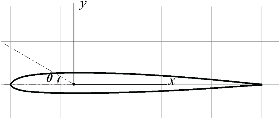
Figure 1: Research subject wing type

2.2 Wind Tunnel Testing and Numerical Methodology for Dynamic Stall

The dynamic stall experiments were conducted in a high-speed continuous wind tunnel, which inflow Mach number is in the range of 0.1–1.3. The chord length of experimental wing model is 0.21 m, while the span length is 0.6 m. A position servo-control system governed the airfoil’s pitching oscillations, where the servo-motor executed predefined non-uniform rotational motions through a motion control card. Twenty-seven dynamic pressure transducers were distributed along the upper and lower surfaces to acquire unsteady pressure data. Real-time synchronized voltage sampling at 50 kHz enabled phase-locked integration of surface pressures over multiple oscillation cycles, followed by periodic averaging to extract high-fidelity unsteady aerodynamic forces and moments. Detailed specifications of the experimental apparatus, measurement protocols, and data processing procedures are documented in References [16,17].

The low-fidelity unsteady aerodynamic data were obtained by solving two-dimensional compressible unsteady Reynolds-averaged Navier-Stokes (URANS) equations coupled with the Menter’s shear stress transport (SST) k-ω turbulence model [18]. The governing equations were discretized using a cell-centered finite volume method with the following numerical schemes:

•   Temporal discretization: Second-order implicit dual-time stepping

•   Inviscid fluxes: Second-order upwind scheme with Roe’s approximate Riemann solver

•   Viscous fluxes: Second-order central differencing

A sliding mesh technique (Fig. 2) was implemented to resolve the pitching motion, where the near-field grid rotated synchronously with the airfoil while maintaining connectivity with the stationary background mesh. The computational domain extended 20 chord lengths radially, with far-field boundaries employing characteristic-based pressure conditions and airfoil surfaces modeled as no-slip adiabatic walls.

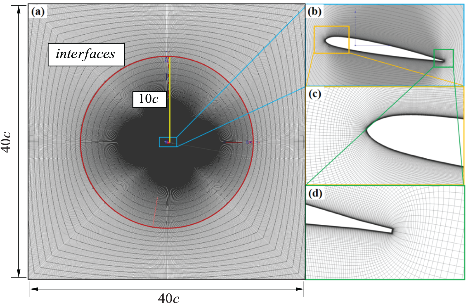
Figure 2: Flowfield Simulation Grid. (a) whole simulation domain (b) grid around airfoil (c) grid around leading edge of airfoil (d) grid around trailing edge of airfoil

2.3 Co-Kriging Model for Multi-Fidelity Surrogate Modeling

For an m-dimensional problem, suppose we are concerned with the prediction of an expensive-to-evaluate (and unknown) function yS1:Rm→R with assistance of a cheaper-to-evaluate function yS2:Rm→R (extension to multiple levels of fidelity is straightforward). Two computer codes of different fidelity are run to get two data sets, which are sampled at the sites

{S1=[x1(1)x1(2)⋅⋅⋅x1(n1)]T∈Rn1×mS2=[x2(1)x2(2)⋅⋅⋅x2(n2)]T∈Rn2×m(2)

here, n1 and n2 are the number of sampling sites for the high- and low-fidelity computations, respectively; usually n2≫n1. x=[ReMa]T with the corresponding responses.

{yS1=[y1(1)y1(2)⋅⋅⋅y1(n1)]T=[y(x1(1))y(x1(2))⋅⋅⋅y(x1(n1))]T∈Rn1yS2=[y2(1)y2(2)⋅⋅⋅y2(n1)]T=[y(x2(1))y(x2(2))⋅⋅⋅y(x2(n2))]T∈Rn2(3)

The Co-Kriging model prediction is defined as:

y^(x)=ωTyS=∑i=1n1ω1(i)yS1(i)+∑i=1n2ω2(i)yS2(i)=ω1TyS1+ω2TyS2(4)

where ω1 and ω2 are the weighting coefficients for high- and low-fidelity responses, respectively. Assuming two stationary random processes corresponding to y1 and y2:

{Y1(x)=β1+Z1(x)Y2(x)=β2+Z2(x)(5)

The covariance and cross-covariance between random variables at different locations in the design space are defined as:

{Cov[Z(x1(i)),Z(x1(j))]=σ12R(11)(x1(i),x1(j))Cov[Z(x2(i)),Z(x2(j))]=σ22R(22)(x2(i),x2(j))Cov[Z(x1(i)),Z(x2(j))]=σ1σ2R(12)(x1(i),x2(j))(6)

here, σ12 and σ22 represent the process variances of the random processes Y1(x) and Y2(x), respectively.

The Co-Kriging model aims to find optimal weighting coefficients ω1 and ω2 that minimize the mean squared error (MSE):

MSE[y^(x)]=E[(ω1TyS1+ω2TyS2−Y1(x))2](7)

subject to the interpolation (unbiasedness) constraint:

E[ω1TyS1+ω2TyS2]=E[Y1(x)](8)

To solve this constrained minimization problem, the weighting coefficients in Eq. (4) are determined via the following linear system (Co-Kriging equations):

[C(11)C(12)10C(21)C(22)011T0T000T1T00][ω1ω2μ1/2μ2/2]=[c1(x)c2(x)10](9)

where μ={μ1,μ2}T is the vector of Lagrange multipliers, 1 is a column vector of ones, and other matrices are defined as:

C(11)=(σ12R(11)(x1,i,x1,j))i,j∈Rn1×n1,C(12)=(σ1σ2R(12)(x1,i,x2,j))i,j=(C(21))T∈Rn1×n2,C(22)=(σ22R(22)(x2,i,x2,j))i,j∈Rn2×n2,c1=(σ12R(11)(x1,i,x))i∈Rn1,c2=(σ1σ2R(12)(x2,i,x))i∈Rn2(10)

To eliminate σ1 and σ2 from the covariance matrices, parameter transformations are applied to the weighting coefficients and Lagrange operators:

ω∼1=ω1,ω∼2=σ2/σ1ω2μ∼1=μ1/(2σ12),μ∼2=μ2/(2σ1σ2)(11)

This constitutes a critical definition in the Co-Kriging model. Substituting Eq. (11) into Eq. (9) yields:

[R(11)R(12)10R(21)R(22)011T0T000T1T00][ω∼1ω∼2μ∼1μ∼2]=[r1(x)r2(x)10](12)

with correlation matrices defined as:

R(11)=(R(11)(x1,i,x1,j))i,j∈Rn1×n1,R(12)=(R(12)(x1,i,x2,j))i,j=(R(21))T∈Rn1×n2,R(22)=(R(22)(x2,i,x2,j))i,j∈Rn2×n2,r1=(R(11)(x1,i,x))i∈Rn1,r2=(R(12)(x2,i,x))i∈Rn2(13)

After solving for the new weights ω∼1 and ω∼2, the Co-Kriging prediction can be reformulated as:

y^1(x)=(ω∼1)Ty1+σ1σ2(ω∼2)Ty2(14)

or in matrix form:

y^1(x)=[r1(x)r2(x)10]T[R(11)R(12)10R(21)R(22)011T0T000T1T00][y1σ1σ2y200](15)

By inverting the block matrix in Eq. (15), the Co-Kriging predictor becomes analogous to the model proposed by Sacks et al. [19]:

y^1(x)=φTβ∼+rT(x)R−1(y∼S−Fβ∼)(16)

where the matrices are defined as:

{φ=[10],β∼=[β∼1β∼2]=(FTR−1F)−1FTR−1y∼Sr=[r1(x)r2(x)],R=[R(11)R(12)R(21)R(22)]y∼S=[yS1σ1σ2yS2],F=[1001]∈R(n1+n2)×2(17)

With the above formulae, β∼, σ1/σ2 and σ12 can be found by maximizing the concentrated ln likelihood function (neglecting constant terms), Parameters θ obtained by numerical optimization method [20].

Based on the critical definitions in Eq. (11) and the unbiasedness constraint in Eq. (8), the root mean squared error (RMSE) of the Co-Kriging model is derived as:

MSE{y^(x)}=σ12[1−rTR−1r+(φ−FTR−1r)⋅(FTR−1F)−1(φ−FTR−1r)T(18)

2.4 Interval Uncertainty Quantification Method and Sensitivity Analysis

Building upon the multi-fidelity surrogate model established in Section 2.3, interval uncertainty quantification analysis was conducted. Let X=[XL,XU] represent the uncertainty interval of independent variables, which can be expressed as:

X=Xc+[−1,1]Xd(19)

where Xc=(XL+XU)/2 and Xd=(−XL+XU)/2, denoting the uncertainty level of the variable x. The independent variables can then be expressed as:

{x=Xc+xdxd∈[−1,1]Xd(20)

For dependent variables y^1=f(x)=f(Xc+xd)∈Y=[YL,YU], a first-order Taylor expansion about Xc yields:

{YL≈f(Xc)−|∂y^1∂x|XdYU≈f(Xc)+|∂y^1∂x|Xd(21)

The resultant uncertainty in Y becomes:

Yd=(YU−YL)/2=|∂y^1∂x|Xd(22)

The total variance D of the dependent variable can be decomposed into contributions from individual random variables:

D=∑i=1NDi+∑1≤i<j≤NDij+⋅⋅⋅+D1,2,⋯,N(23)

The relative sensitivity of random variables (Reynolds/Mach numbers) to dependent variables (aerodynamic forces/moments) is quantified through Sobol indices. Sobol indices are calculated as the ratio between the variance of individual random variables and the total variance:

Si1,⋯,is=Di1,⋯,is/D(24)

3  Case Validation and Results Analysis

3.1 Case Validation

3.1.1 Validation of Dynamic Stall Numerical Methodology

Gardner et al. [21] conducted wind tunnel tests on the OA209 airfoil’s dynamic stall characteristics in a transonic wind tunnel within the Mach number range of 0.3–0.5, obtaining comprehensive unsteady aerodynamic data. To validate the numerical methodology described in Section 2.2, simulations were performed at Ma = 0.31 and Re = 1.2 × 106 under identical kinematic conditions. The computational results were systematically compared with experimental data to validate the reliability of the numerical methodology:

•   Mean angle of attack: θ0=12.5deg

•   Pitching amplitude: Aθ=7.5deg

•   Oscillation frequency: fθ=5.7Hz

•   Pivot location: 1/4 chord position

A grid independence study was conducted using three distinct mesh configurations (Table 1).

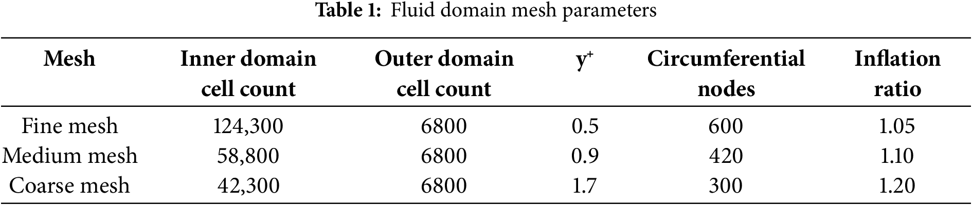
Fig. 3 compares the dynamic stall lift coefficient hysteresis loops computed using three different meshes with experimental data. The results demonstrate that the unsteady lift coefficients obtained through the numerical methodology employed in this study exhibit strong agreement with experimental measurements, with discrepancies primarily observed during the airfoil downstroke phase. In the downstroke phase, computational results show delayed flow reattachment compared to experimental data. This discrepancy arises because the numerical simulations neglect disturbance factors present in experiments, such as surface roughness on the test model, wind tunnel wall interference, and inflow turbulence. These experimental factors enhance turbulent kinetic energy production, accelerating flow reattachment. The increased error bars in experimental data during downstroke (see Fig. 3) further confirm the flow’s heightened sensitivity to environmental perturbations in this phase. Furthermore, the figure reveals negligible differences between medium and fine mesh results, while coarse mesh predictions deviate noticeably. Considering the balance between computational efficiency and accuracy, the medium-resolution mesh was selected for subsequent analyses. Meanwhile, this dynamic stall numerical method also be validated using other dynamic stall cases, which can be found in our previous studies [22,23].

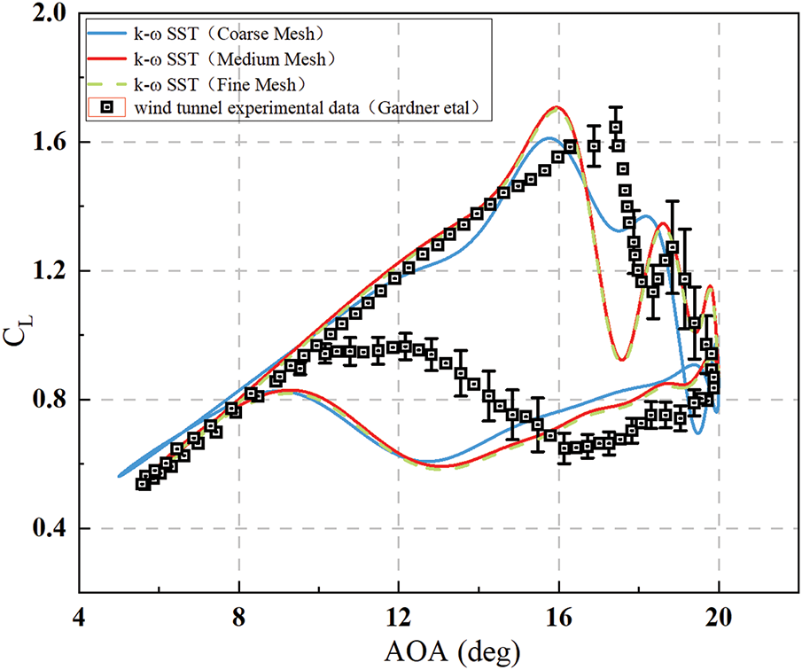
Figure 3: Dynamic stall lift coefficient hysteresis curve

3.1.2 Multi-Fidelity Surrogate Model Validation

The multi-fidelity surrogate model sampling points are shown in Fig. 4, where red markers represent wind tunnel test cases and blue markers denote numerical simulation cases sampled via a full factorial experimental design method. The Mach number varies within 0.1~0.6, and the Reynolds number ranges from 2.6 × 105~5 × 106. The unsteady aerodynamic forces/moments of dynamic stall vary over a pitching oscillation cycle. These forces are discretized into m equal time intervals per cycle, with each interval divided into temporal elements of duration T/m. Co-Kriging-based multi-fidelity surrogate models were constructed for aerodynamic forces at the mid-interval timestamp of each temporal element. Validation was performed using withheld high-fidelity data (Ma = 0.35, Re = 3 × 106), with results presented in Fig. 5. The predictions from the multi-fidelity surrogate model demonstrate errors within 5% compared to high-fidelity data, confirming the model’s reliability.

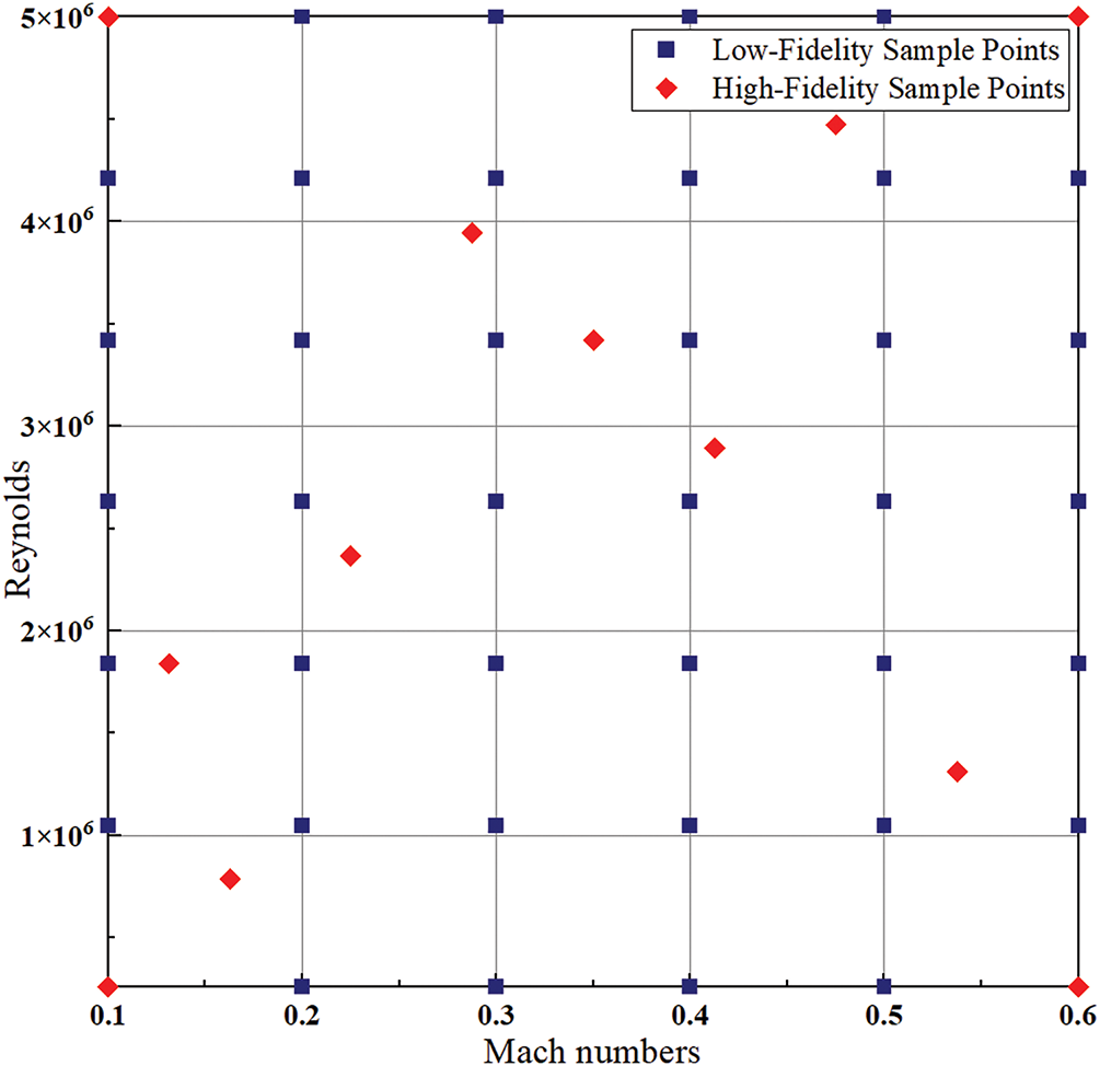
Figure 4: Sample points for modeling multi-fidelity agents

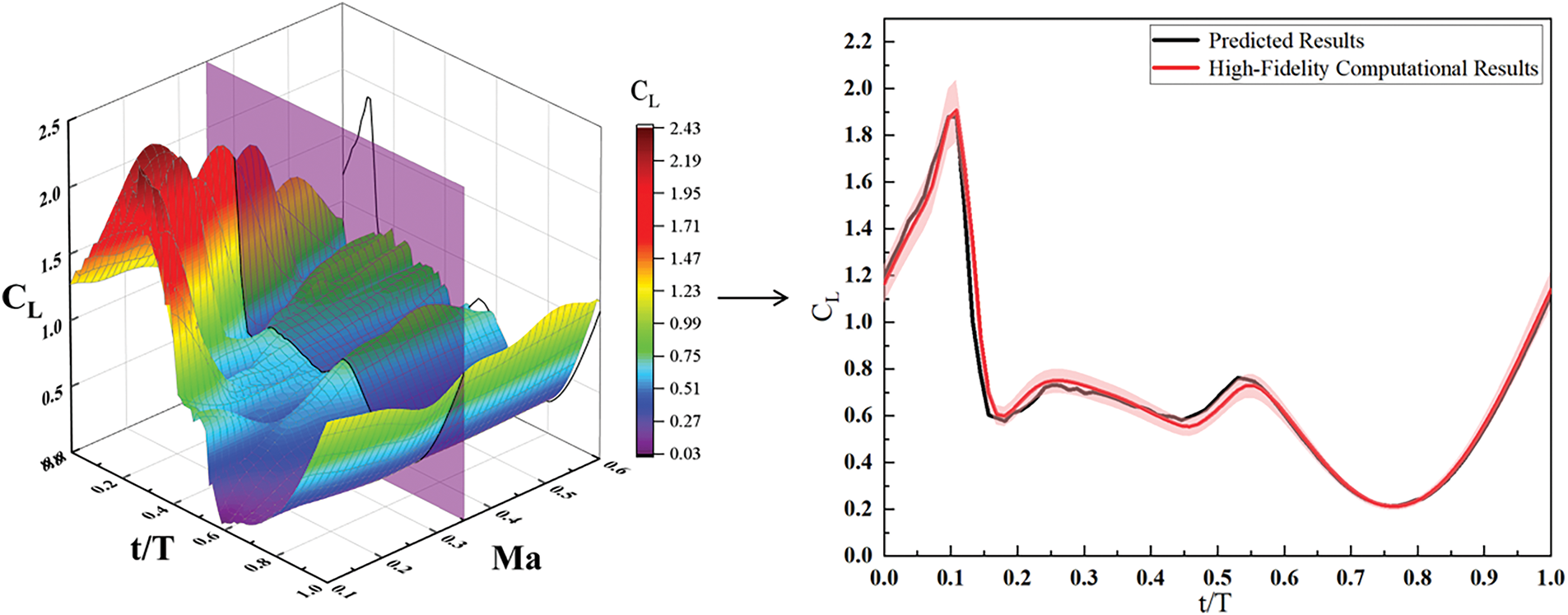
Figure 5: Multi-fidelity surrogate model predictions vs. high-fidelity data

3.2 Uncertainty Quantification Results

This section selects the inflow Reynolds number and Mach number as uncertain variables, with nominal values of 4 × 106 and 0.5, respectively, both with 10% uncertainty. The 10% uncertainty indicates Xd=10%Xc. Specifically, while the Mach number is nominally set at 0.5, actual values may fluctuate within a range of 0.45–0.55. Similarly, the Reynolds number could vary between 3.6 × 106 and 4.4 × 106.

Fig. 6 shows the effects of Mach number and Reynolds number on the uncertainties of aerodynamic forces/moments at different time instances. It is evident that the influence of Mach number on the uncertainty of unsteady aerodynamic forces and moments is significantly greater than that of Reynolds number. When Ma < 0.3, the compressibility effect is weak without any shock, so the trailing-edge separation is mainly induced by the adverse pressure gradient, which leads to the light dynamic stall. As shown in Fig. 7, the compressibility effect increases, and a local supersonic region appears near the leading edge when Ma ≥ 0.3. Besides, as the Mach number increases, the local supersonic region and shock intensity increases, and the local supersonic region and dynamic stall vortex forms in an earlier phase of the pitch motion. The much earlier appearance of local supersonic region and dynamic stall vortex in the upstroke leads to the severe dynamic stall. Therefore, as shown in Fig. 5, the peak value of lift reduces significantly as the Mach number increases.

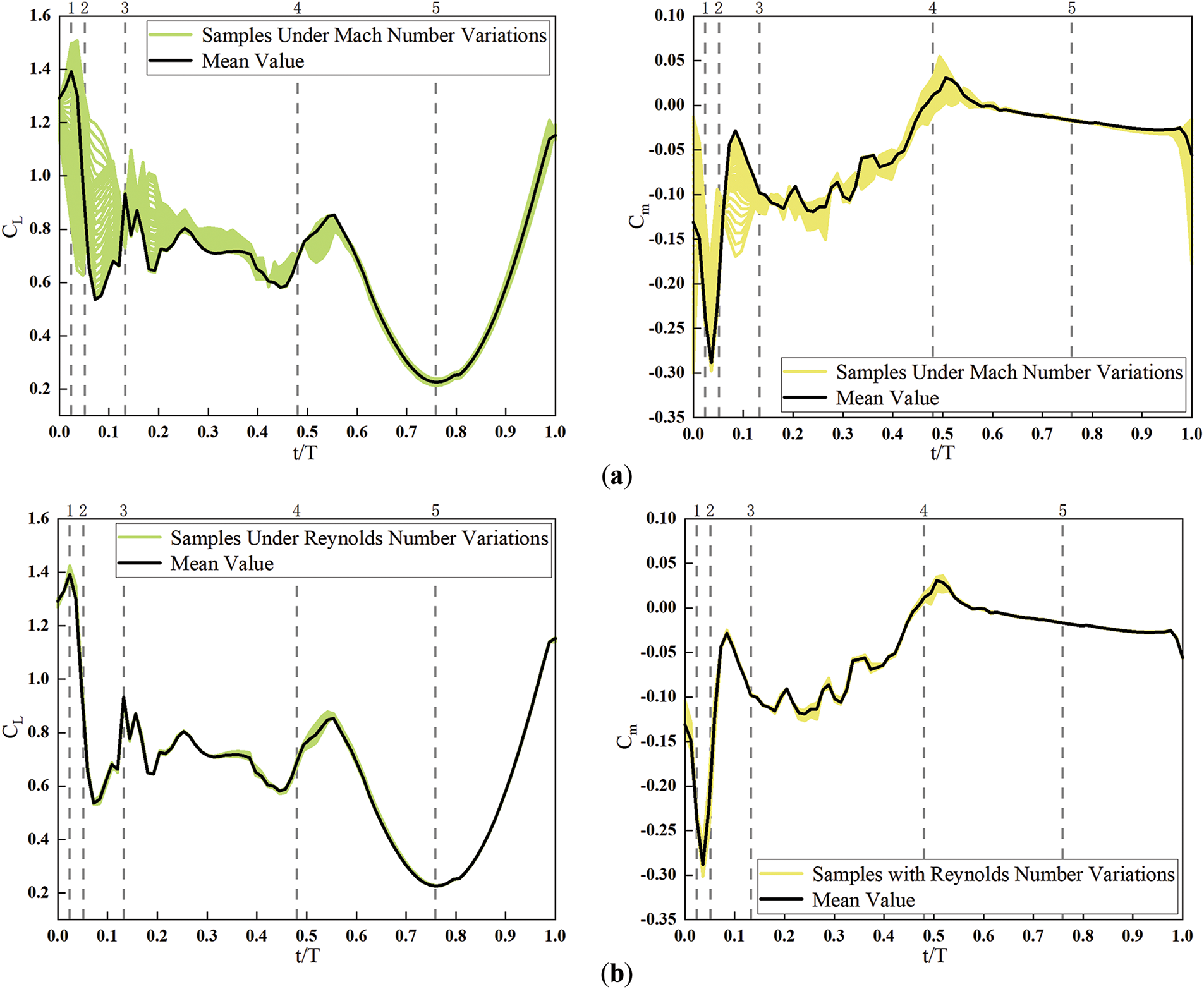
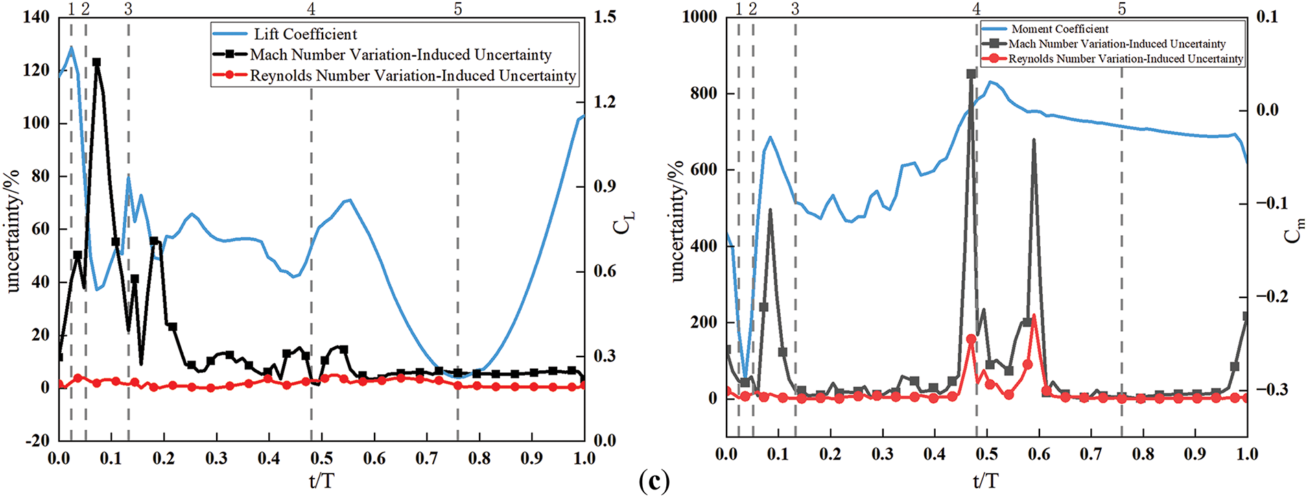
Figure 6: Effect of Mach number and Reynolds number uncertainty on aerodynamic forces/moments at different moments. (a) Samples with Mach Number Variations; (b) Samples with Reynolds Number Variations; (c) Uncertainty in Lift Coefficient/Moment Coefficient. The ranges of Mach number and Reynolds number studied in this figure are detailed in the first paragraph of Section 3.2. The horizontal axis t/T represents the normalized time over one pitching cycle, corresponding to distinct phases of the pitching motion

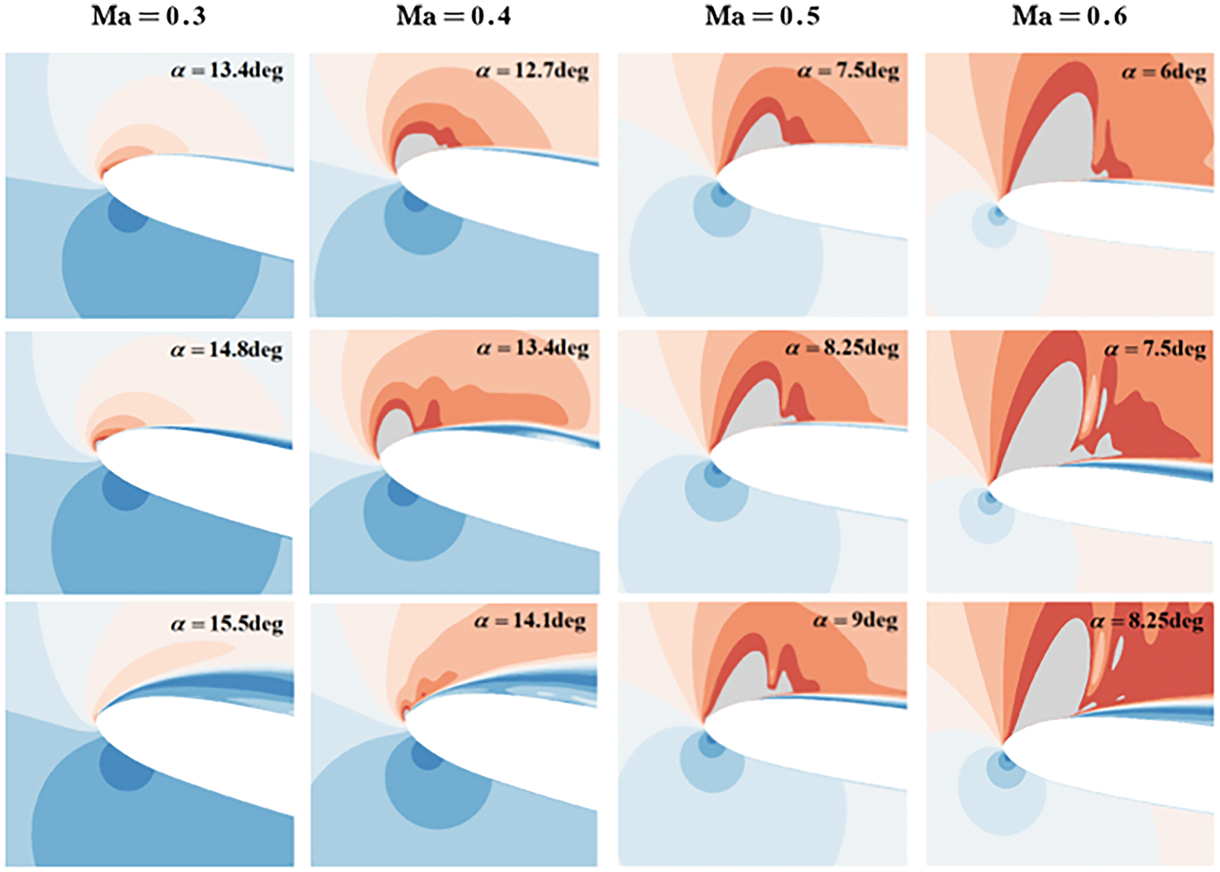
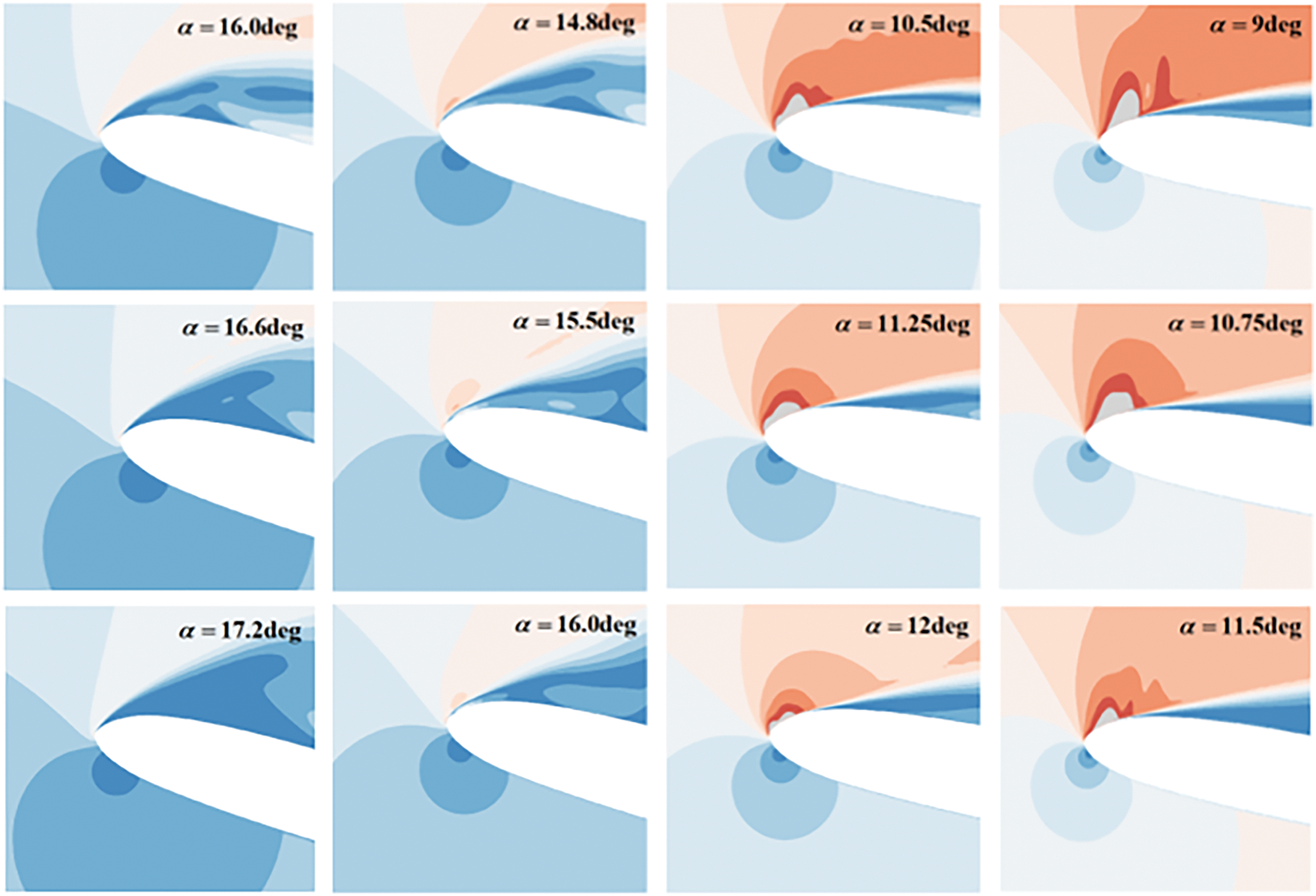
Figure 7: Mach field around the pitching airfoil under different inlet Mach numbers. The supersonic field is indicated by the grey color

Table 2 presents the uncertainties in aerodynamic forces/moments induced by Mach and Reynolds numbers at several critical flow states. The flow state is based on the fluid field results at the nominal values of Reynolds number (Re = 4 × 106) and Mach number (Ma = 0.5). The results indicate that larger uncertainties occur during the dynamic stall vortex generation, downstream movement along the upper airfoil surface, and shedding phases. Notably, the Mach number-induced uncertainty in lift coefficient exhibits a peak at the dynamic stall vortex shedding location. This phenomenon arises from two factors:

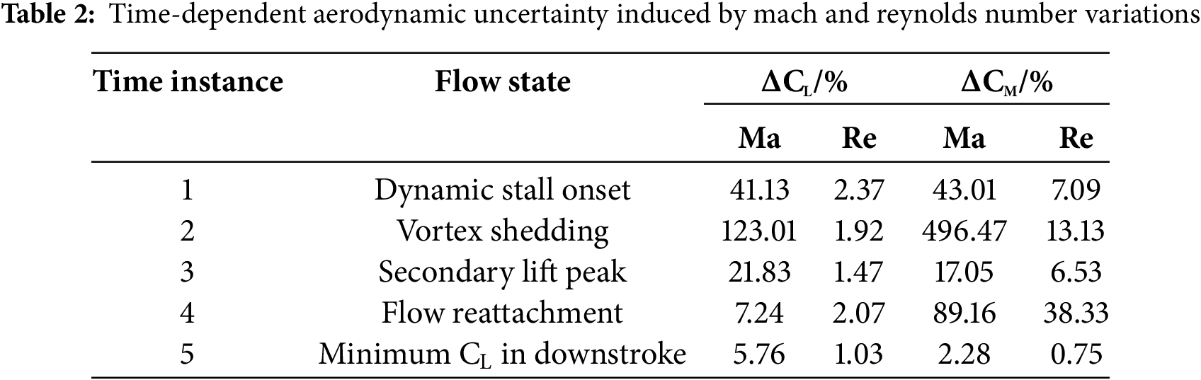
1.   The appearance phase and size of leading-edge supersonic region under different Mach numbers affects the evolution process of the dynamic stall vortex. At the nominal Mach number, the dynamic stall vortex has completely shed, while at smaller Mach numbers, the vortex continues to convect downstream along the airfoil surface, generating substantial lift uncertainty.

2.   The uncertainty is referenced to the mean position, which coincides with the minimum lift coefficient point during the upstroke phase.

In contrast, lower uncertainties are observed during the airfoil downstroke phase, where fluctuations in Mach and Reynolds numbers practically do not induce variations in aerodynamic forces/moments.

Fig. 8 presents the sensitivity analysis results of Mach and Reynolds numbers on dynamic stall aerodynamic characteristics. It is evident that the sensitivity of lift/moment coefficients to Mach number is significantly higher than to Reynolds number. From Fig. 6a, it can be observed that the nominal Mach value frequently resides in extreme states, with transitions between extreme states occurring near certain time instances. This results in a significant reduction of Mach number-induced uncertainty at those moments, causing the sensitivity of lift coefficient to Reynolds number to exceed that to Mach number at these specific times, with similar behavior observed for the moment coefficient.

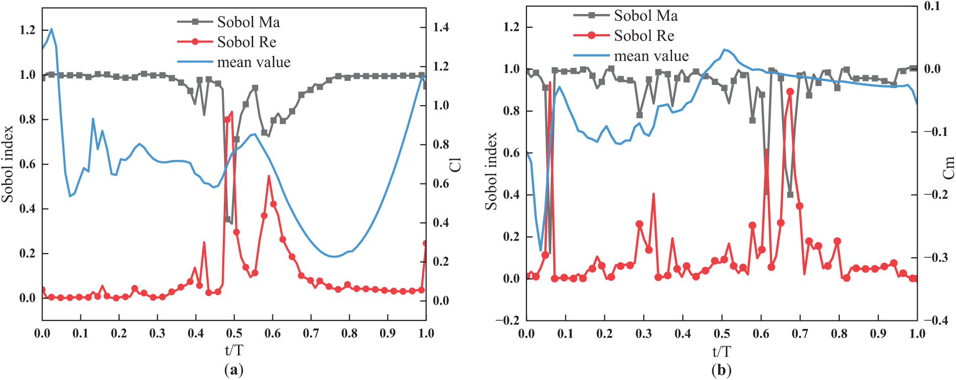
Figure 8: Sensitivity analysis of Mach number and Reynolds number of dynamic stall aerodynamic characteristics. (a) Lift Coefficient; (b) Moment Coefficient. The Mach number ranges from 0.45 to 0.55, and the Reynolds number ranges from 3.6 × 106 to 4.4 × 106. The definition of Sobol index can be found in Eq. (24)

From the flow mechanism perspective: The relatively large nominal Reynolds number eliminates transition phenomena observed in related studies, rendering aerodynamic characteristics insensitive to Reynolds number variations. The nominal Mach number often lies at critical thresholds where leading-edge supersonic regions initiate. The interaction between emerging supersonic zones and dynamic stall vortices alters vortex evolution processes, leading to extreme sensitivity of aerodynamic characteristics to Mach number variations—particularly when dynamic stall vortices exist in the flow field.

4  Conclusions

This study investigated a two-dimensional airfoil section through combined wind tunnel testing and numerical simulations to acquire multi-fidelity unsteady aerodynamic data. A Co-Kriging-based multi-fidelity surrogate model was developed for dynamic stall aerodynamic characteristics. Interval analysis and Sobol methods were subsequently employed to conduct uncertainty quantification and parameter sensitivity analysis, yielding the following conclusions:

1.   The unsteady Reynolds-averaged Navier-Stokes (URANS) numerical methodology demonstrates satisfactory prediction accuracy for dynamic stall aerodynamic characteristics. However, discrepancies between numerical results and high-fidelity experimental data occur during the downstroke phase due to unmodeled disturbance factors in simulations, including surface roughness, wind tunnel wall interference, and inlet turbulence;

2.   The Co-Kriging multi-fidelity surrogate model achieves high predictive accuracy, with errors below 5% compared to high-fidelity data;

3.   Mach number uncertainty exerts significantly greater influence on unsteady aerodynamic forces/moments than Reynolds number variations. This effect amplifies substantially when dynamic stall vortices exist in the flow field. As the Mach number increases, the compressibility effect grows, and the larger area and much earlier appearance of local supersonic region leads to the severe dynamic stall. Therefore, the compressibility effect induced by inlet Mach number uncertain leads to much uncertainty of lift, especially near the peak value.

Acknowledgement: The authors sincerely thank the honorable referees and the editor for their valuable comments and suggestions, which have significantly improved the quality of this paper.

Funding Statement: The authors received no specific funding for this study.

Author Contributions: Yizhe Han: Writing—original draft, Methodology, Visualization, Formal analysis. Guangjing Huang: Writing—review & editing, Validation, Methodology. Fei Xiao: Visualization, Investigation. Zhiyin Huang: Conceptualization, Software, Supervision. Yuting Dai: Writing—review & editing, Investigation, Supervision. All authors reviewed the results and approved the final version of the manuscript.

Availability of Data and Materials: The data that support the findings of this study are available upon reasonable request from the authors.

Ethics Approval: Not applicable.

Conflicts of Interest: The authors declare no conflicts of interest to report regarding the present study.

References

1. Corke TC, Thomas FO. Dynamic stall in pitching airfoils: aerodynamic damping and compressibility effects. Annu Rev Fluid Mech. 2015;47(1):479–505. doi:10.1146/annurev-fluid-010814-013632. [Google Scholar] [CrossRef]

2. Gardner AD, Jones AR, Mulleners K, Naughton JW, Smith MJ. Review of rotating wing dynamic stall: experiments and flow control. Prog Aerosp Sci. 2023;137(1):100887. doi:10.1016/j.paerosci.2023.100887. [Google Scholar] [CrossRef]

3. Zhu C, Yang H, Qiu Y, Zhou G, Wang L, Feng Y, et al. Effects of the Reynolds number and reduced frequency on the aerodynamic performance and dynamic stall behaviors of a vertical axis wind turbine. Energy Convers Manag. 2023;293(1):117513. doi:10.1016/j.enconman.2023.117513. [Google Scholar] [CrossRef]

4. Benton SI, Visbal MR. The onset of dynamic stall at a high, transitional Reynolds number. J Fluid Mech. 2019;861:860–85. doi:10.1017/jfm.2018.939. [Google Scholar] [CrossRef]

5. Lee S, Chanez B, Gross A. Numerical analysis of Reynolds and Mach number effect on dynamic stall onset. Phys Fluids. 2024;36(11):1–17. doi:10.1063/5.0239448. [Google Scholar] [CrossRef]

6. Faes M, Moens D. Recent trends in the modeling and quantification of non-probabilistic uncertainty. Arch Comput Methods Eng. 2020;27(3):633–71. doi:10.1007/s11831-019-09327-x. [Google Scholar] [CrossRef]

7. Oladyshkin S, Nowak W. Data-driven uncertainty quantification using the arbitrary polynomial chaos expansion. Reliab Eng Syst Saf. 2012;106(1):179–90. doi:10.1016/j.ress.2012.05.002. [Google Scholar] [CrossRef]

8. Huang R, Qiu Z. Interval analysis method for uncertain aerodynamic loads computation. J Beijing Univ Aeronaut Astronaut. 2013;39(4):525–30. doi:10.13700/j.bh.1001-5965.2013.04.026. [Google Scholar] [CrossRef]

9. Song X, Zheng G, Yang G, Jiang Q. Interval analysis for geometric uncertainty and robust aerodynamic optimization design. J Beijing Univ Aeronaut Astronaut. 2019;45(11):2217–27. doi:10.13700/j.bh.1001-5965.2019.0077. [Google Scholar] [CrossRef]

10. Kaya H, Tiftikçi H, Kutluay Ü., Sakarya E. Generation of surrogate-based aerodynamic model of an UCAV configuration using an adaptive co-Kriging method. Aerosp Sci Technol. 2019;95:105511. doi:10.1016/j.ast.2019.105511. [Google Scholar] [CrossRef]

11. Marepally K, Jung YS, Baeder J, Vijayakumar G. Uncertainty quantification of wind turbine airfoil aerodynamics with geometric uncertainty. J Phys Conf Ser. 2022;2265(4):042041. doi:10.1088/1742-6596/2265/4/042041. [Google Scholar] [CrossRef]

12. Wu X, Zhang W, Song S. Uncertainty quantification and sensitivity analysis of transonic aerodynamics with geometric uncertainty. Int J Aerosp Eng. 2017;2017(1):8107190. doi:10.1155/2017/8107190. [Google Scholar] [CrossRef]

13. Deng X, Chen Q, Yuan X, Chen J. Study of aerodynamic uncertainty on the complex slender vehicle at high angle of attack. Sci Sin (Technol). 2016;46(5):493–9. [Google Scholar]

14. Chen X, Wang G, Ye ZY, Wu X. A review of uncertainty quantification methods for computational fluid dynamics. Acta Aerodyn Sin. 2021;39(4):1–13. doi:10.7638/kqdlxxb-2021.0012. [Google Scholar] [CrossRef]

15. Xia Z, Luo J. Uncertainty quantification of inlet incidence angle variation for turbine blade. J Aerosp Power. 2020;35(3):519–31. doi:10.13224/j.cnki.jasp.2020.03.008. [Google Scholar] [CrossRef]

16. Li G, Zhang W, Chen L, Nie B, Zhang P, Yue T. Research on dynamic test technology for wind turbine bland airfile. Chin J Theor Appl Mech. 2018;50(4):751–65. doi:10.6052/0459-1879-18-108. [Google Scholar] [CrossRef]

17. Li G, Song K, Qin C, Zhao G, Wu L, Yang Y. Test on active control of airfoil dynamic stall based on trailing edge flap. Acta Aeronaut Et Astronaut Sin. 2024;45(3):110–25. doi:10.7527/S1000-6893.2023.28699. [Google Scholar] [CrossRef]

18. Menter FR. Two-equation eddy-viscosity turbulence models for engineering applications. AIAA J. 1994;32(8):1598–605. doi:10.2514/3.12149. [Google Scholar] [CrossRef]

19. Sacks J, Welch WJ, Mitchell TJ, Wynn HP. Design and analysis of computer experiments. Stat Sci. 1989;4(4):409–23. doi:10.1214/ss/1177012413. [Google Scholar] [CrossRef]

20. Gaspar B, Teixeira AP, Soares CG. Assessment of the efficiency of Kriging surrogate models for structural reliability analysis. Probabilistic Eng Mech. 2014;37(2–3):24–34. doi:10.1016/j.probengmech.2014.03.011. [Google Scholar] [CrossRef]

21. Gardner AD, Richter K, Mai H, Altmikus AR, Klein A, Rohardt CH. Experimental investigation of dynamic stall performance for the EDI-M109 and EDI-M112 airfoils. J Am Helicopter Soc. 2013;58(1):1–13. doi:10.4050/jahs.58.012005. [Google Scholar] [CrossRef]

22. Wu Y, Dai Y, Yang C, Hu Y, Huang G. Effect of trailing-edge morphing on flow characteristics around a pitching airfoil. AIAA J. 2023;61(1):160–73. doi:10.2514/1.j061055. [Google Scholar] [CrossRef]

23. Xia Y, Dai Y, Huang G, Yang C. Stall flutter mitigation of an airfoil by active surface morphing. Phys Fluids. 2024;36(8):1–17. doi:10.1063/5.0222902. [Google Scholar] [CrossRef]