Unmanned Aerial Vehicle Assisted Forest Fire Detection Using Deep Convolutional Neural Network

1  Introduction

Forest fire is one of the most dangerous natural disasters in the world. Various factors have contributed to increased wildfire frequency and destruction, including a more extended average season, warming weather that aggravates vulnerability, and early melting of winter snowpacks caused by global climate change [1]. According to a recent study, fire departments across the United States need to react to a fire somewhere in the nation almost every twenty seconds [2]. A different study showed that, in April 2020, the number of fire warnings increased by 13% globally compared to the previous year [3], and 6803 fires were identified only in the Amazon during July 2020 [4]. Among the fire occurrences, forest fires are the most consequential. It creates a substantial CO2 imbalance, decimates biodiversity, affects economies, endangers livelihoods, and causes severe health issues worldwide [5].

Consequently, around 0.55 million people had to be relocated throughout the globe due to forest fires only in 2017 [6]. However, the consequences of wildfires continue to affect in the longer term. An estimated 0.34 million people died from premature deaths from respiratory and cardiovascular diseases connected to wildfire [7]. Moreover, the burgeoning number of wildfire occurrences creates a severe global threat to biodiversity. For example, in 2019–20 in Australia, the catastrophic wildfires killed or displaced around 3000 million animals. Notably, many of the animals in that Australian occurrence were vulnerable classes like koalas [8].

Moreover, the financial losses due to the increased number of fire occurrences are rapidly soaring. The estimated global loss of wildfire was around $52 trillion from 1984 to 2013 [9], while only in 2018 did the USA spend about $50 billion to combat forest fire [10]. Additionally, the total forest loss in the first half of 2020 was 307,000 hectares, 26% higher than in 2019 [11]. Consequently, from the Arctic to the Amazon, severe fires contributed 20% of the global carbon emissions in 2019 [12].

Thus, a scientific approach is necessary to combat the proliferation of wildfire to achieve sustainable development goals (SDGs). By developing new detection technologies and taking proper measures, it is possible to bring the loss to a minimum. For this purpose, we need to build a real-time monitoring system of fire activity, especially in the forest area and share this information immediately with the authorities. Those monitoring systems will integrate multiple technologies, including unmanned aerial vehicles (UAV)/satellite, Internet-of-Things (IoT), Cloud/Fog computing infrastructure, and wireless communication networks. Specifically, UAVs can perform extensive services, covering drone delivery to surveillance and monitoring [13]. Additionally, UAV’s versatility, autonomy, and deployability render them suitable to be a part of the forest fire surveillance, detection, and control system. Also, economically, UAVs are relatively cheaper compared to satellite surveillance.

Over the recent years, researchers have been focusing on developing state-of-the-art technology and algorithms for forest fire detection [14]. Those researches are continuously adding to the advancement in this field. However, the existing model’s performances focused on a limited number of evaluation metrics and scope. Also, due to the limited availability of standard and benchmark datasets, these studies used diverse data sources, making a straightforward comparison quite tricky. Considering the weaknesses of previous research, we have proposed a CNN-based classification model in this article. Herein, we assessed its performance with multiple evaluation metrics for robust and reliable outcomes, describing each step of the methodology and the model’s architecture.

The remainder of the paper is organized as follows. Section 2 discusses related research on forest fires. Section 3 then describes the employed methodology and short discussions on its building blocks. Section 4 shows the obtained results and briefly explains the outcomes where necessary. Finally, Section 5 presents a summary of the work done in this paper and potential directions for future research in this field.

2  Related Work

Muhammad et al. investigated four different models for fire detection [15]. In their investigation, they used a pre-trained AlexNet CNN model. According to their problem domain, they fine-tuned it to detect fire in various indoor and outdoor environments, achieving 94.39% accuracy. The same authors proposed an improvement of their work, where a SqueezeNet architecture-inspired CNN architecture yielded a computationally efficient & lightweight architecture [16]. They fine-tuned their CNN architecture to detect fire in different indoor and outdoor environments and localize it in their improved work. As a result, their model achieved 94.50% accuracy, 0.11% more than the previous model.

In 2018, They proposed another CNN-based architecture by fine-tuning the GoogleNet, where they tried to balance the efficiency and accuracy of the model [17]. They showed that their model could detect the fire properly even though video frames can be affected by noise or contain a small fire. Although the model’s accuracy has increased comparatively, the false alarm rate is still high. In 2019, Muhammad et al. proposed an efficient CNN-based method for fire detection approach in an uncertain IoT environment on the captured video frame [18]. They used lightweight deep neural networks without applying dense, fully connected layers to ensure less computational complexity and storage. The experimental result showed that their model was dominant with the state-of-art method with 95.86% accuracy. In 2019, Saeed et al. proposed a fire detection method based on powerful machine learning and deep learning algorithms. They used Adaboost and Multilayer Perceptron (MLP) neural networks, an Adaboost-LBP model, and a convolution neural network similar to AlexNet with slight changes on a dataset consisting of both sensors data and images data that contains different fire scenarios [19]. They achieved almost 99% accuracy with a lower false alarm rate than the traditional CNN model. Sharma et al. proposed a fire detection method based on a Deep CNN. They used VGG16 and Resnet50 on a self-made dataset consisting of images taken from the internet, which are difficult to classify and highly unbalanced by including fewer fire images than nonfire images [20]. They achieved 90.19% accuracy from VGG16% and 91.18% accuracy from Resnet50. After modifying both models by adding fully connected layers, which helped to improve the accuracy of VGG16 and Resnet50 91.18% and 92.15%, respectively.

In 2017, Maksymiv et al. proposed a real-time fire detection method combining Adaboost, Local binary pattern (LBP), and a customized CNN classifier [21]. The combination of Adaboost and LBP is used to get areas of interest to reduce the proposed model’s time complexity. It is vital to have a large and balanced dataset to make a CNN-based model efficient and generalized. Otherwise, there is a chance of falling into the trap of an overfitting problem. In 2021, Song et al. [22] proposed an outdoor fire recognition technique where they worked on a small dataset. They improved DC-GAN to generate more data to tackle the shortage and unbalanced problem. After solving unbalanced fire images, they have applied transfer learning on pre-trained MobileNet to classify fire and non-fire images. Finally, the Experiment result showed the improvement of model accuracy by 0.9251, reducing the overfitting problem. In 2021, Shamsoshoara et al. proposed a fire detection method for pine forests [23] and achieved 76% test accuracy. In 2021, J. Zhang et al. proposed an adequate fire detection Technique called ATT Squeeze U-Net, where they incorporated a modified SqueezeNet structure into Attention U-Net architecture [24]. This novel approach assisted them in achieving 93% accuracy and prediction time at 0.89 s per image. In 2020 Pu Li et al. proposed novel fire detection techniques by fine-tuning advanced object detection CNN models, which are Faster-RCNN [25], R–FCN [26], SSD [27], and YOLO v3 [28] on a large dataset [29]. Those proposed object detection models can automatically extract complex image fire features that help detect fire in different scenes. Comparative results among those object detection models show that the average precision based on YOLO v3 is 83.7%, which is higher than the other proposed algorithms with a more substantial detection rate of 28 FPS.

In 2021, Dutta et al. proposed a forest fire detection method using the Separable Convolution and Image Processing technique [30]. The purpose of using the Image processing technique was to handle the smoke and fog issue. This proposed architecture achieved 98.10% sensitivity (recall) and 87.09% specificity. Fire changes its shape under the influence of wind and its burning nature. Based on those phenomena, in 2019, Wu et al. proposed a fire detection technique [31]. In 2019, Pan et al. proposed a time-efficient forest fire detection Network called AddNet. They used a multiplication-free vector operator that performs only addition and sign manipulation operations [32]. They got a 95.6% actual detection rate using this custom architecture. In 2020, Rahul et al. proposed a CNN-based method for early forest fire detection by fine-tuning ResNet50, adding some convolutional layers with ReLu Activation functions for their binary classification [33]. They conducted their experiment using CNN-based models like VGG16, ResNet50, and DenseNet121, but they got satisfactory results from ResNet50. They achieved 92.27% training accuracy with 89.57% test accuracy. Besides, CNN-based models are being utilized in different areas [34–37].

3  Methodology

This section describes the methodology of our proposed work. Fig. 1 illustrates the complete scenario of the proposed Forest Fire Management System. Initially, the proposed model will be developed through the training and testing from the selected forest dataset, which contains Fire and Non-Fire scenes. After the training, the model’s reliability and effectiveness will be checked by observing the quantitative results of the test data. After achieving satisfactory model performance, the trained model will be installed in the UAV for real-time fire detection. This UAV is then deployed and maintained by the forest department through the wireless communication network. The UAV can capture the real-time image from the forest and produce the fire or non-fire outcome with the help of the proposed model. This outcome is communicated to the data center by the UAV through the communication system. If the data center gets the fire signal, it finally informs the disaster management system to take the necessary steps to control the fire.

Figure 1: Forest fire management system

If there is any fire on the captured image, then an alarm will be transmitted to the fire department. Otherwise, the surveillance UAV will continue to roam. Initially, we have focused on building the Fire detection model (depicted at Top-Left in Fig. 1), which will be installed in UAV for surveillance purposes. In Fig. 2, we have shown our Workflow for creating the Fire detection Model. This work proposes an autonomous forest fire detection system based on examining forest scenes and extracting features from them using a customized CNN architecture. A set of Forest Fire images, including both the fire and non-fire scenes, is required for training the supervised learning model. These images were taken from a recently published dataset (described in Section 3.1).

Figure 2: Workflow of the proposed method

First and foremost, the images were augmented. Then the images were split as Train (80%) and Test (20%) samples. Before sending the Train samples into the Model, they have been normalized (from 0 to 1) to make the training process faster. Next, the suggested CNN model has been trained using the Normalized Train samples. Finally, Normalized Test samples were used to evaluate the CNN Model.

3.1 Data Collection

The detection performance largely depends on the data on which it is trained. However, there is no single benchmark dataset for fire detection. We have used a recently published dataset named ‘Dataset for Forest Fire Detection from Mendeley Data to train and test our fire detection model [38].

Fig. 3 shows sample fire and non-fire images of the dataset. The dataset contains RGB images with a resolution of 250 × 250 pixels. The authors of [38] collected those images from different sources by applying different search patterns. After collecting those images, a few images were cropped or deleted depending on their condition. Finally, the authors created a balanced dataset comprised of 1900 (Fire and non-fire) images, where each of the classes contains 950 images.

Figure 3: Fire and non-fire images of dataset

3.2 Data Augmentation

CNN-based Machine learning algorithms require many data to avoid overfitting issues [39]. Data Augmentation is a helpful technique to enlarge a dataset that assists a model in learning a function with comparatively low variance. According to our problem domain, we have performed a horizontal flip on each image. The idea behind image flipping is that an image should be as recognized as its mirror version. Horizontal flipping is the most common sort of flipping. Vertical flipping is not usually a good idea, but it depends on the situation. This augmentation process has been applied to the whole dataset and doubled the number of images. This brings the total number of train images to 3800. Fig. 4 illustrates the result of the augmentation process. The following equation can represent the horizontal flipping operation.

Oij={Ii,O.cols−j−1 (1)

where, I, O, i, and j are, respectively, an Input image, output image, indexing of row, and indexing of column of the matrix of image.

Figure 4: Sample images before and after augmentation

3.3 Normalization

Normalization is helpful data preprocessing technic which is helpful for training and testing a CNN model. In the dataset that has been used all the pixels of each image contain RGB (Red, Green, and Blue) colors have an intensity value ranging from 0 to 255. We have rescaled our input data in a range between 0 and 1.

xi′=xi−xminxmax−xmin (2)

where, xi, and xi′ are input data and output data while xmin and xmax are the minimum (0) and maximum (255) possible value of input data respectively.

3.4 CNN and its Layers

CNN performs a wide range of Computer Vision tasks. Over the years, CNN has enabled numerous researchers to contribute to the various domains [40,41] and continue to succeed. A CNN is made up of multiple layers, each of which has a task to do when extracting features from input data. The primary components of a CNN are discussed more below.

3.4.1 Convolutional Layer

The convolutional layer is the most significant layer of a CNN model. Convolution operations are needed to generate the relevant feature maps from the input data. Depending on the problem domain, a set of filters is used at a convolutional layer. Each filter has a specific number of parameters, which are learned during the training period. Each filter pulls over the input volume to perform a sum of the dot products between the filter and the current patch of the input image. After completing the convolutional operation with all kernels, it will produce output-feature maps. Generally, those features’ size (width and height) is relatively small compared to the input data. However, it would be possible to get the output feature the same as the input image by applying padding on the border of the input image before the convolution operation. Convolution that involves one-dimensional signal processing is known as simple convolution. It is a convolution commonly used when a convolution action is performed between two signals that span along two dimensions that are mutually orthogonal to one another; the operation is called 2D convolution. CNN can easily be customized to work with the input signal having other sizes. Before conducting a convolution operation, sometimes it may need to apply zero-padding into the input feature based on the problem domain. Zero-padding is a term used in convolutional neural networks to describe the process of wrapping a matrix with zeroes. This can aid in the preservation of features that exist at the borders of the original matrix and the management of the size of the output feature map.

If the Input Image and Filter for convolution are denoted by I ∈ ℝW×H and F ∈ ℝL×M respectively. Then 2-D convolution can be expressed by the following equation [42].

(I∗F)(m,n)=∑i=0L−1∑j=0M−1⁡I(m+i,n+j)F(i,j)m=0,…,H−1,n=0,…,W−1 (3)

Here, W and H are the width and height of the input image (I), while L and M are the Filter’s width and height, respectively.

Using Eq. (3), we can compute the output feature of the input image (I) as (W * L + 1) * (H * M + 1), where each value is computed using the same equation. It is important to note that the stride of the convolution is one, which means that the equation above is performed for every m and n in the matrix of input image I.

Any number of convolutions is feasible based on the size of the input image and the design of the CNN model. A convolution layer contains N filters that, after being applied to the same input image, produce N output features with various patterns.

In Fig. 5, an example of a convolution operation has been shown where stride was one.

Figure 5: Convolution operation

Filter (F) will be moved horizontally as well as vertically through the input Image (I). After the completion of convolution, the output feature (O) has been shown in the Bottom-Right part of the Above Figure. From the figure, the result of the convolution operation on the present patch of input figure by Filter (F) is −8 (multiplication and summation have shown at the top of the output feature). Further calculations have been skipped except the outcome only shown.

Separable Convolutional Operation

Separate Convolution Operation takes place in two steps. The first step is Depthwise Convolution (Fig. 6), and the second step is called Pointwise Convolution (Fig. 7). In the first step, at the time of Depthwise Convolution, D (equal to the number of input channels) number of kernels with the shape of are used. Only one kernel iterates to only one channel of the image. However, the number of multiplications at the first step of separable convolution is evaluated.

a)   Firstly, the Number of Multiplication at the time of single convolution will be K2

b)   Secondly, the Number of Multiplication at the time of a whole convolution on a single channel will be, (M − K − 1) × (M − K − 1) K2

c)   Finally, the Number of Multiplication with each of the D number of channels will be G2K2D.

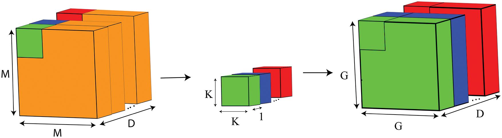
Figure 6: Depthwise convolution

Figure 7: Pointwise convolution

During the second step, Pointwise Convolutions are applied to the result of the Depthwise Convolution (as it takes the result from the previous step as input). The kernel with the shape 1 × 1 × D is used here. However, the number of multiplications required at the second step of separable convolution is as follows.

a)   Firstly, the Number of Multiplication at the time of single convolution will be D.

b)   Secondly, the Number of Multiplication at the time of a whole convolution on input image will be G2D.

c)   Finally, the Number of Multiplication with N kernels will be G2DN

In terms of Separable Convolution, the total number of multiplication will be the summation of the Resulted multiplication from the Depthwise step and Pointwise step. The total Number of multiplication can be denoted as follows:

Mseparable=G2K2D+G2DN=G2D(K2+N) (4)

In terms of Separable Convolutional operation at the first step of Depthwise Convolution, with D number of filters with the shape of K × K × 1, the number of parameters will be K2D. Again, At the phase of Pointwise Convolution N number of Filters with shape 1 × 1 × D, the number of parameters will be ND.

So, Using a Separable Convolutional operation total number of parameters can be denoted as follows:

Pseparable=K2D+ND=D(K2+N) (5)

3.4.2 Activation Function

The output of a convolutional operation is passed through a non-linear function in a neural network. In CNN, the Activation function introduces the non-linearity by transforming the weighted sum of the input of a node used in different layers. According to the functionality, the other Activation function is used in the CNN model to learn and execute complex tasks. Rectified Linear Units (ReLU) do not change the positive inputs, but it maps the negative inputs to zero [43]. The functional property of ReLu is as follows:

f(x)=max(0,x) (6)

3.4.3 Batch Normalization

Ioffe et al. [44] proposed a concept to make the Deep Neural Network training process faster and more stable by re-centering and re-scaling the layer’s input by applying a normalization operation. Batch Normalization is usually used to reduce overfitting. If B denotes a mini-batch of a training dataset with size n at each hidden layer, Batch Normalization transforms the signal as follows:

uB=1n∑i=1nxi (7)

σB=1n∑i=1n⁡(xi−uB) (8)

Here, uB and σB are the mean and standard deviation of the activation values across the mini-batch, respectively. All the layer of a DNN has a fixed D-dimensional input xD[D ∈ |1, d|] and all of the dimensions normalized using the following equation.

xi(norm)(D)=xi(D)−μB(D)σB(D)2+ϵ,i∈[1,m] (9)

where, μB(D) and σB(D) are respectively mean and variance of each dimension. ε is the arbitrary constant used for numerical stability. The final result of the normalization process yi(D) , is calculated by applying a linear transformation with two trainable parameters which are γ(D) and β(D) using the following equation.

yi(D)=γ(D)χi(norm)(D)+β(D) (10)

Adjustment of γ(D) and β(D) allow the model to its optimum distribution for each hidden layer.

3.4.4 Pooling Layer (Downsampling)

The pooling process is done by sliding a two-dimensional filter through each channel of a feature map and then extracting the features from each filter region based on the pooling type. A Pooling layer takes larger-sized feature maps and shrinks them to lower-sized feature maps. The reduction of the feature map also leads to fewer parameters being used in the following layers. Pooling operations allow the model to become more robust by reducing the variance. Multiple pooling techniques are used in the different pooling layers, namely Max pooling, Average pooling, Min pooling, Gated pooling, Tree pooling, etc. Among them, Max pooling and Average pooling are commonly used techniques in CNN.

Fig. 8 shows Max pooling and Average pooling operation. The left side of this figure demonstrates the input feature map with the size of (4 × 4) while the Upper-Right and Lower-Right parts of the figures depict the output feature map with the size of (2 × 2) after conducting the max and average pooling operations respectively. However, both of the pooling operations reduce the size of the input feature map though the max pooling operation focus on maximum value (8, 12, 14, and 22 are the maximum values of the four patches with size (2 × 2) of the input feature) and average pooling calculates the mean value (5, 8, 7 and 19 are the mean values of the four patches with size (2 × 2) of the input feature).

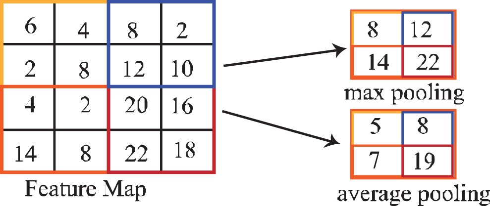
Figure 8: Max and average pooling operation

3.4.5 Flatten Layer

A CNN model has two parts, namely feature extraction and classification. A Flatten layer usually lies between these two parts in a CNN model. The Feature extractor part usually outputs a three-dimensional tensor. On the other hand, the classifier is nothing but an artificial neural network (ANN) that expects a one-dimensional input for prediction purposes. A Flatten layer transforms a tensor into a vector that the following dense layers can interpret. This type of transformation is known as flattening.

3.4.6 Fully Connected Layers

A fully connected (FC) layer is a layer where each element/node of a layer is connected to each element of the following layer. Output at any node in a fully connected layer depends on the neurons of the immediately previous layer. A network with multiple fully connected layers between the input and output layers is often referred to as a Deep network. Each neuron of an FC layer has an activation function. Relu is the most used nonlinear activation function used in the fully connected layers. The number of FC layers and their neurons depend on the problem domain and complexity of the Dataset. The total number of neurons of the final FC layer corresponds to the number of classes of the Dataset. Softmax activation is usually used in the last FC Layer to perform that classification task as it maps a vector of numbers into a vector of probabilities.

3.5 Proposed Architecture

Fig. 9 illustrates the architecture of the proposed model. All the operations and layers used in the model have been marked differently. The size of the input image shape is 250 × 250 with three RGB color channels. Before passing, the input data (images) into the designed model has been normalized to make the training process faster and more efficient. The standard convolutional operation was conducted in the initial part of the architecture (as the number of initially used feature maps was less). The number of filters is 16, and each of those filters has a dimension of 3 × 3. This layer provides 16 feature maps with a size of 83 × 83. Following this layer, Relu activation was performed. Finally, Max Pooling has been performed to downsample the size of the feature maps. Then Depthwise separable convolution operation was performed using 32-separable convolutional layers sized 3 × 3. This operation produces 32 feature maps of size 27 × 27 with fewer parameters. The activation function was then called as usual, and finally, Max Pooling was performed to downsample the size of the feature maps. This separable convolution operation was performed twice. Using separable convolution twice, the feature map size was reduced to 9 × 9. Later, two consecutive separable convolutional operations were conducted where 64-filters were used. An activation operation is also conducted after every convolutional operation. The Bach normalization layer was used to normalize the weight of the model. After that Max pooling operation was conducted to get 64 feature maps sized 4 × 4, this type of arrangement helps extract the same number of features with a lower computational cost. After performing the flatten operation, three fully connected (FC) layers were used for classification purposes, where the first two FC layer’s sizes were the same (128) with a 30% dropout, and the last FC layer’s size was 64 with a 20% dropout to handle overfitting problems. Before applying Dropout, Batch Normalization was performed. Finally, to maintain the number of output classes (fire and non-fire), two dense layers are added to the proposed network with a softmax activation function according to our classification problem.

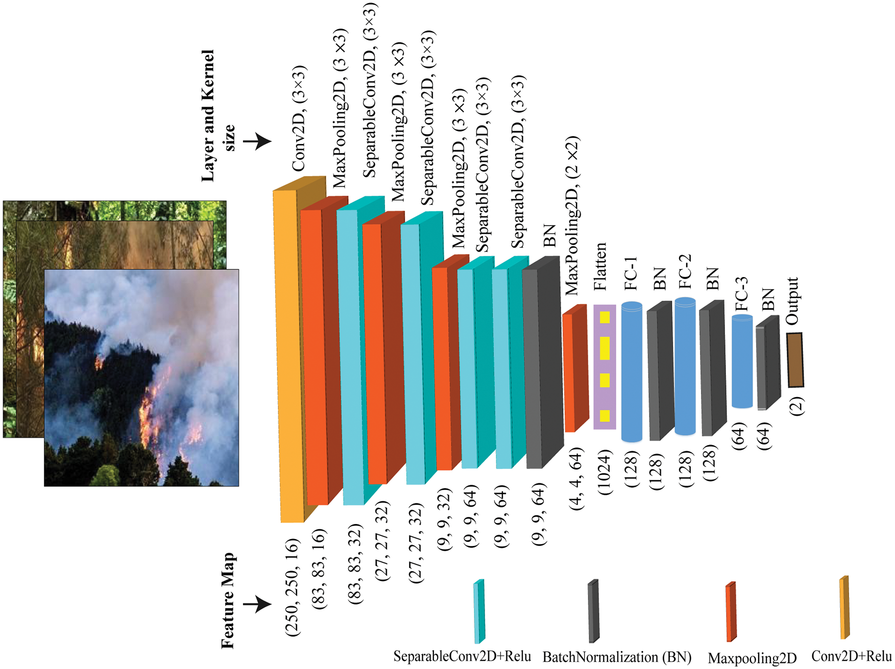
Figure 9: Proposed model architecture

One thing is to mentionable that at the all convolutional stage we have the same padding and unit stride of the filters as we do not want to lose the border element and also relevant information of the input image.

4  Results and Discussion

In this section, we illustrate the effectiveness of the model we have proposed by using several well-known metrics. Hyper-parameters that have been used in our proposed model are presented in Tab. 1, with their associated value. We have used Google collab with free GPU (NVIDIA Tesla K80), Intel(R) Xeon(R) CPU (2.20 GHz), and Tensorflow (Version-2.8.0) for our experiment. By examining all of these metrics, we arrived at excellent and acceptable results for our model.

4.1 Performance Evaluation with Existing Fire Detection Models

In this subsection, we performed a classification task for forest fire detection. This section presents the achieved results of the classification process with discussions and compares the model’s performance with concurrent methods in this field. As we stated in Section 3, we have trained our model (depicted in Fig. 9.) with 80% samples of the total dataset and evaluated it with the rest of 20% samples. We analyzed our model’s performance based on well-known evaluation metrics, including classification accuracy, precision, recall, F1-Score, Quadratic Weighted Kappa (QWK), and confusion matrix. We trained the proposed model for 150 epochs. Fig. 10a shows the corresponding accuracy values for both the train and test stages at each epoch. Accuracy is the most commonly used evaluation metric while using a balanced dataset. As we can see, the curve of the training process increased smoothly as the epochs increased. However, the test accuracy curve had a few zig-zags initially, which can be understood from its abrupt change at the initial epochs. Nevertheless, it got stable after the 140th epoch. At the last epoch, the train and test accuracies are 99.9% and 96.4%, respectively, indicating the model’s superior performance. However, we got the highest test accuracy (97.6%) at the 120th epoch. The mean and standard deviation of the last 10th trains and test epochs were approximately 96.5% and 0.004%, respectively, which indicates the model achieved its stability Figs. 10b and 10c depicts the precision and recall, while Fig. 11a depicts the F1-Score curves for the train and test phases based on their respective epochs. These metrics are very effective in judging a model thoroughly. Precision reveals the percentage of true positive samples instead of the total number of samples identified as positive (for a particular class). When a model predicts something, its authenticity is verified with the recall value. The recall is the percentage of identified positive samples identified correctly by the model. The F1-Score is a harmonic mean of precision and recall scores. A high F1-Score increases the model’s acceptability. From Figs. 10b, 10c and 11a, we can check the model’s reliability and unbiasedness by looking at the train and test phase’s precision, recall, and F1-Score curves. All of these curves are pretty similar to their corresponding accuracy curves.

Figure 10: Model analysis matrics-1

Figure 11: Model analysis matrics-2

Another reliable evaluation metric is the QWK, a chance-adjusted metric used to judge the performance of the classification model. If the value of QWK is more than 80%, then it is deemed to be a perfect agreement between qualitative items. Fig. 11b shows a plot of the QWK values concerning each epoch. The highest QWK score on the test set is 95.3%, which was achieved in the 120th epoch. Finally, Fig. 11c shows the Confusion matrix of the best epoch where most test data are correctly categorized. According to the models prediction, True positive rate (TPR),True negative rate (TNR), false-positive rate (FPR) and false-negative rate (FNR) are 97.89%, 97.37%, 2.63%, and 2.11% respectively. These results also claim the model’s high performance and admissibility.

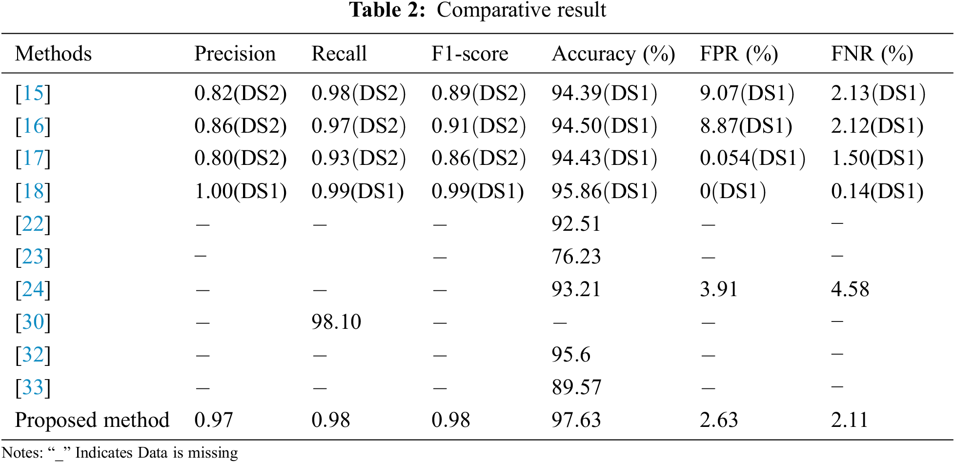
Tab. 2 shows the comparative result of the proposed work with other related classification methods on fire detection. Our approach has achieved competitive results compared to others methods. The dataset we used to train the proposed method was recently published, so the result of the proposed method is not directly comparable with the other cited methods. All the studies mentioned in the table are relatively recent (published between 2017 and 2021). We considered accuracy, precision, recall, and F1-Score to compare the result of the methods. Table entity with ‘−’ refers that the particular information is missing. In [15–18], the authors used two datasets to evaluate their method, DS1 and DS2. They used DS2 to determine the precision, recall, F1-Score, and DS1 to determine accuracy, FPR, and FNR in [15–17]. Tab. 2 represents only the best outcome of [18] on DS1. Based on recall, precision, and F1-Score, the method applied in [18] achieved the highest position, but its accuracy (95.86%) is still lower than the accuracy of the proposed method. Our model’s performance is the best based on the accuracy since its accuracy (97.63%) is the highest among the mentioned methods. Besides, the precision of the proposed model is 97% which is the second-highest in the entire comparison table. Our proposed method also showed a high F1-Score, and recall. This discussion concludes that the proposed method’s performance is reliable and authentic for accurate forest fire detection. However, further improvement is needed to decrease the FPR and FNR.

4.2 Computational Time of Simulation

Our proposed CNN architecture is computationally efficient due to the use of separable convolutional layers requiring less computation and fewer parameters. In terms of training the 3040 images, the execution time was 728.723 s (whereas it takes 1101.096 s when using standard convolutional layers at different model stages).

4.3 Performance Evaluation with Existing Fire Detection Models

We have implemented some existing and recent CNN models built to detect Forest Fires. By following the proper instructions of that exemplary architecture [22,23,45,46], we have to build those models on our own. Then, we trained those created models with 3040 images. Finally, the Performance of those models is analyzed based on Accuracy, Precision, and Recall using 760 images.

As shown in Tab. 3, we have compared the performance of our model with those of existing fire detection models. From the table, it was evident that the proposed model outperforms those existing fire detection models. From the above table, we can see the highest accuracy is 97.63% which the proposed fire detection model achieves. Our proposed model also gains the highest precision value compared to other models. Also, the Recall is the maximum of our model compared to others.

Our model’s performance is spectacular, evidenced by the well-known metrics listed above. The high value of those indicators assures our model’s suitability for identifying forest fires. As a result, when combined with a UAV, this fire detection model has the potential to be a highly successful tool in reducing and even preventing severe damage caused by wildfires.

5  Conclusion

A forest fire is often an unforeseen event that can cause substantial damage to plants, forest wildlife, and other properties within a short time. This paper proposed an image-based fire detection technique using a Deep CNN model combining convolutional and separable convolutional layers. We implemented our model on a recent fire detection dataset, and experimental results showed that the proposed method performed well compared with state-of-the-art methods. Moreover, the proposed method achieved higher accuracy (97.63%), precision, and lower FPR and FNR than the existing ones. Our future work will be the development of our methods by which the current limitations of the model can be overcome to make it more suitable for actual use. We will experiment with different forests in different geological regions. We’ll concentrate our efforts on expanding our research into fire detection at night and day. We will try to integrate the implemented CNN Model into the UAV to check the effectiveness of our proposed management system. We will also focus on UAV path planning and efficient allocation to ensure flawless surveillance at a low cost.

Funding Statement: Princess Nourah bint Abdulrahman University Researchers Supporting Project Number (PNURSP2022R54), Princess Nourah bint Abdulrahman University, Riyadh, Saudi Arabia.

Conflicts of Interest: The authors declare that they have no conflicts of interest to report regarding the present study.

References

 1.  Climate Change Indicators: Wildfires, United States Environmental Protection Agency, 2021. [Online]. Available: https://www.epa.gov/climate-indicators/climate-change-indicators-wildfires. [Google Scholar]

 2.  M. Ahrens and B. Evarts, “Fire loss in the United States,” NFPA report, 2021. [Online]. Available: https://www.nfpa.org/News-and-Research/Data-research-and-tools/US-Fire-Problem/Fire-loss-in-the-United-States. [Google Scholar]

 3.  S. McCarthy, in 2020 Forest Fires Globally could be Worse than 2019, WWF Warns, WWF-Press Releases, 2020. [Online]. Available: https://www.worldwildlife.org/press-releases/2020-forest-fires-globally-could-be-worse-than-2019-wwf-warns. [Google Scholar]

 4.  WWF-Brazil, “Pantanal also requires attention: The biome is the champion of increased fire in 2020,” August 2020. [Online]. Available: https://wwf.panda.org/wwf_news/?462751/amazonfire2020. [Google Scholar]

 5.  FORESTS ABLAZE, “Causes and effects of global forest fires. WWW study,” 2017. [Online]. Available: https://www.wwf.de/fileadmin/fm-wwf/Publikationen-PDF/WWF-Study-Forests-Ablaze.pdf. [Google Scholar]

 6.  GFMC, “Recent media highlights on fire, policies, and politics,” February 2007. [Online]. Available: https://gfmc.online/media/2007/02-2007/news_feb.html. [Google Scholar]

 7.  F. H. Johnston, S. B. Henderson, Y. Chen, J. T. Randerson, M. Marlier et al., “Estimated global mortality attributable to smoke from landscape fires,” Environmental Health Perspectives, vol. 120, no. 5, pp. 695–701, 2012. [Google Scholar]

 8.  P. Mercer, “Australia ‘facing hotter future’,” BC NEWS, January 2004. [Online]. Available: https://gfmc.online/media/2004/bbc-news-asia-pacific-australia-facing-hotter-future.html. [Google Scholar]

 9.  S. H. Doerr and C. Santín, “Global trends in wildfire and its impacts: Perceptions versus realities in a changing world,” Philosophical Transactions of the Royal Society B: Biological Sciences, vol. 371, no. 1696, pp. 20150345, 2016. [Google Scholar]

10. P. Howard, “Flammable planet: Wildfires and the social cost of carbon,” no. September, pp. 45, 2014, [Online]. Available: http://costofcarbon.org/files/Flammable_Planet__Wildfires_and_Social_Cost_of_Carbon.pdf. [Google Scholar]

11. H. Escobar, “Brazilian institute head fired after clashing with nation’s president over deforestation data,” Science (1979), 2019. https://doi.org/10.1126/SCIENCE.AAY9857. [Google Scholar]

12. L. M. Lombrana, H. Warren and A. Rathi, “Measuring the carbon-dioxide cost of last year’s worldwide wildfires,” Bloomberg, February 2020. [Online]. Available: https://www.bloomberg.com/graphics/2020-fire-emissions/. [Google Scholar]

13. M. Mozaffari, A. T. Z. Kasgari, W. Saad, M. Bennis and M. Debbah, “Beyond 5G with UAVs: Foundations of a 3D wireless cellular network,” IEEE Transactions on Wireless Communications, vol. 18, no. 1, pp. 357–372, 2019. [Google Scholar]

14. C. Yuan, Y. Zhang and Z. Liu, “A survey on technologies for automatic forest fire monitoring, detection, and fighting using unmanned aerial vehicles and remote sensing techniques,” Canadian Journal of Forest Research, vol. 45, no. 7, pp. 783–792, 2015. [Google Scholar]

15. K. Muhammad, J. Ahmad and S. W. Baik, “Early fire detection using convolutional neural networks during surveillance for effective disaster management,” Neurocomputing, vol. 288, pp. 30–42, 2018. [Google Scholar]

16. K. Muhammad, J. Ahmad, Z. Lv, P. Bellavista, P. Yang et al., “Efficient deep CNN-based fire detection and localization in video surveillance applications,” IEEE Transactions on Systems, Man, and Cybernetics: Systems, vol. 49, no. 7, pp. 1419–1434, 2019. [Google Scholar]

17. K. Muhammad, J. Ahmad, I. Mehmood, S. Rho and S. W. Baik, “Convolutional neural networks based fire detection in surveillance videos,” IEEE Access, vol. 6, pp. 18174–18183, 2018. [Google Scholar]

18. K. Muhammad, S. Khan, M. Elhoseny, S. H. Ahmed and S. W. Baik, “Efficient fire detection for uncertain surveillance environment,” IEEE Transactions on Industrial Informatics, vol. 15, no. 5, pp. 3113–3122, 2019. [Google Scholar]

19. F. Saeed, A. Paul, P. Karthigaikumar and A. Nayyar, “Convolutional neural network based early fire detection,” Multimedia Tools and Applications, vol. 79, no. 13, pp. 9083–9099, 2019. [Google Scholar]

20. J. Sharma, O. C. Granmo, M. Goodwin and J. T. Fidje, “Deep convolutional neural networks for fire detection in images,” Communications in Computer and Information Science, vol. 744, pp. 183–193, 2017. [Google Scholar]

21. O. Maksymiv, T. Rak and D. Peleshko, “Real-time fire detection method combining AdaBoost, LBP and convolutional neural network in video sequence,” in 2017 14th International Conf. the Experience of Designing and Application of CAD Systems in Microelectronics, CADSM 2017-Proc., pp. 351–353, May 2017. [Google Scholar]

22. X. Song, S. Gao, X. Liu and C. Chen, “An outdoor fire recognition algorithm for small unbalanced samples,” Alexandria Engineering Journal, vol. 60, no. 3, pp. 2801–2809, 2021. [Google Scholar]

23. A. Shamsoshoara, F. Afghah, A. Razi, L. Zheng, P. Z. Fulé et al., “Aerial imagery pile burn detection using deep learning: The FLAME dataset,” Computer Networks, vol. 193, pp. 108001, 2020. [Google Scholar]

24. J. Zhang, H. Zhu, P. Wang and X. Ling, “ATT squeeze U-net: A lightweight network for forest fire detection and recognition,” IEEE Access, vol. 9, pp. 10858–10870, 2021. [Google Scholar]

25. S. Ren, K. He, R. Girshick and J. Sun, “Faster R-CNN: Towards real-time object detection with region proposal networks,” IEEE Transactions on Pattern Analysis and Machine Intelligence, vol. 39, no. 6, pp. 1137–1149, 2017. [Google Scholar]

26. J. Dai, Y. Li, K. He and J. Sun, “R-FCN: Object detection via region-based fully convolutional networks,” Advances in Neural Information Processing Systems, pp. 379–387, 2016. [Google Scholar]

27. W. Liu, D. Anguelov, D. Erhan, C. Szegedy, S. Reed et al., “SSD: Single shot MultiBox detector,” Lecture Notes in Computer Science (Including Subseries Lecture Notes in Artificial Intelligence and Lecture Notes in Bioinformatics), vol. 9905 LNCS, pp. 21–37, 2015. [Google Scholar]

28. J. Redmon and A. Farhadi, “YOLOv3: An incremental improvement,” Apr. 2018, https://doi.org/10.48550/arxiv.1804.02767. [Google Scholar]

29. P. Li and W. Zhao, “Image fire detection algorithms based on convolutional neural networks,” Case Studies in Thermal Engineering, vol. 19, pp. 100625, 2020. [Google Scholar]

30. S. Dutta and S. Ghosh, “Forest fire detection using combined architecture of separable convolution and image processing,” in 2021 1st Int. Conf. on Artificial Intelligence and Data Analytics, CAIDA 2021, Riyadh, Saudi Arabia, pp. 36–41, Apr. 2021. [Google Scholar]

31. H. Wu, D. Wu and J. Zhao, “An intelligent fire detection approach through cameras based on computer vision methods,” Process Safety and Environmental Protection, vol. 127, pp. 245–256, 2019. [Google Scholar]

32. H. Pan, D. Badawi, X. Zhang and A. E. Cetin, “Additive neural network for forest fire detection,” Springer, vol. 14, no. 4, pp. 675–682, 2020. [Google Scholar]

33. M. Rahul, K. S. Saketh, A. Sanjeet and N. S. Naik, “Early detection of forest fire using deep learning,” in 2020 IEEE Region 10 Conf. (TENCON), Osaka, Japan, pp. 1136–1140, 2020. [Google Scholar]

34. M. Masud, N. Sikder, A. -A. Nahid, A. K. Bairagi and M. A. AlZain, “A machine learning approach to diagnosing lung and colon cancer using a deep learning-based classification framework,” Sensors, vol. 21, no. 3, pp. 748, 2021. [Google Scholar]

35. K. Bansal, A. Singh, S. Verma, N. Z. Jhanjhi, M. Shorfuzzaman et al.,” “Evolving CNN with paddy field algorithm for geographical landmark recognition,” Electronics, vol. 11, no. 7, pp. 1075, 2022. [Google Scholar]

36. P. Jain, P. Chawla, M. Masud, S. Mahajan and A. K. Pandit, “Automated identification algorithm using CNN for computer vision in smart refrigerators,” Computers Materials & Continua, vol. 71, no. 2, pp. 3337–3353, 2022. [Google Scholar]

37. V. S. Sharma, K. K. Nagwanshi and G. R. Sinha,” “Classification of defects in photonic bandgap crystal using machine learning under microsoft AzureML environment,” Multimed Tools, pp. 1–16, Appl 2022. https://doi.org/10.1007/s11042-022-11899-z. [Google Scholar]

38. A. Khan and B. Hassan, “Dataset for forest fire detection,” vol. 1, 2020, https://doi.org/10.17632/GJMR63RZ2R.1. [Google Scholar]

39. C. Shorten and T. M. Khoshgoftaar, “A survey on image data augmentation for deep learning,” Journal of Big Data, vol. 6, no. 1, pp. 1–48, 2019. [Google Scholar]

40. N. Baghel, U. Verma and K. K. Nagwanshi, “WBCs-Net: Type identification of white blood cells using convolutional neural network,” Multimedia Tools and Applications, 2021, pp. 1–17, 2021. [Google Scholar]

41. M. H. Khan, N. B.-Jahangeer, W. Dullull, S. Nathire, X. Gao et al., “Multi- class classification of breast cancer abnormalities using deep convolutional neural network (CNN),” PLOS ONE, vol. 16, no. 8, pp. e0256500, 2021. [Google Scholar]

42. H. H. Aghdam and E. J. Heravi, “Guide to convolutional neural networks,” New York, NY: Springer, vol. 10, no. 978–973, pp. 51, 2017, https://doi.org/10.1007/978-3-319-57550-6. [Google Scholar]

43. A. M. Fred Agarap, “Deep learning using rectified linear units (ReLU),” Mar 2018 [Online]. Available: https://github.com/AFAgarap/relu-classifier. [Google Scholar]

44. S. Ioffe and C. Szegedy, “Batch normalization: Accelerating deep network training by reducing internal covariate shift,” in 32nd Int. Conf. on Machine Learning, ICML 2015, Lille, France, vol. 1, pp. 448–456, 2015. [Google Scholar]

45. K. He, X. Zhang, S. Ren and J. Sun, “Deep residual learning for image recognition,” in Proc. of the IEEE Computer Society Conf. on Computer Vision and Pattern Recognition, Las Vegas, NV, USA, vol. 2016-Decem, pp. 770–778, Dec. 2016. [Google Scholar]

46. Z. Zhong, M. Wang, Y. Shi and W. Gao, “A convolutional neural network-based flame detection method in video sequence,” Signal, Image and Video Processing, vol. 12, no. 8, pp. 1619–1627, 2018. [Google Scholar]