A Non-singleton Type-3 Fuzzy Modeling: Optimized by Square-Root Cubature Kalman Filter

1  Introduction

Modeling and identification are essential in various applications. In many cases, it is required that a mathematical model be obtained for a signal. This model can be used in control systems, forecasting problems, protection issues, performance assessment, reverse engineering, etc. In most cases, just some noisy measured data sets are available, and robust modeling systems and learning algorithms are needed to deal with high-level uncertainties and construct an accurate model.

Machine learning (ML) techniques are widely used for forecasting and modeling problems. In [1], radiation forecasting is studied by NNs and SVM techniques. In [2], the forecasting of supply chain demand is studied by an ML approach based on recurrent NNs. In [3], the forecasting of building energy is considered, and the presented methods in the literature are reviewed and classified. The COVID-19 forecasting is investigated in [4], and the superiority of the ML methods is shown. In [5], deep NNs and SVM methods are used for heat load forecasting, and the better accuracy of ML methods is investigated [6] suggests an ML method based on the Boltzmann Machine for Alzheimer’s forecasting. Time series forecasting is studied in [7] by NNs and SVMs. The electrical load forecasting by bagged-boosted NNs is studied in [8], and the excellent performance of ML methods against conventional methods is shown. In [9], tunnel settlement forecasting is taken into account, a backpropagation NN optimized by PSO is presented, and ML techniques’ effectiveness is proved. The ML techniques are extended for tourist arrivals furcating in [10], and the ability of the ML methods are validated on Beijing city tourist arrivals. The blood supply prediction is investigated in [11], using NNs, and ML methods. Literature review shows that ML methods are extensively used for forecasting problems; however, CO2 solubility based on developed ML techniques has been rarely studied. The modeling techniques based on Bayesian NNs are investigated in [12,13], and the performance of Bayesian NNs is examined in driving problems.

Recently, the superiority of the type-2 FLS (T2-FLS) has been shown in ML methods and engineering applications [14]. For example, in [15], the excellent performance of T2-FLS is proved in an energy controller. T2-FLS models the earthquake hazard in [16], and it is shown that the use of T2FLS improves the speed of hazard evaluation. In [17], a power allocation system is designed using T2-FLSs, and network lifetime improvement is shown. The superiority of T2-FLSs in medical diagnosis applications is comprehensively studied in [18]. The image classification method is designed by T2-FLSs in [19], and by several statistical analyses, it is shown that T2FLSs outperform conventional techniques. In [20], the problem of job shop scheduling is studied, and by several comparisons, the better performance of T2-FLSs is demonstrated. The control performance improvement based on T2-FLSs is investigated in [21]. In [22], a microgrid islanding system is designed by T2-FLSs, and the better uncertainty modeling of T2-FLSs is shown. The above review among many other applications of T2-FLSs demonstrates the good capability of FLSs, especially high-order FLSs. Most recently, a developed version of T2-FLSs called interval type-3 FLS has been presented [23]. However, the ML-based method using the T3-FLS approach has been seldom studied. Motivated by the above discussion and review, in this study, a new approach using T3-FLS with non-singleton fuzzification is designed for CO2 solubility modeling and prediction. Furthermore, a new approach is presented for optimization using SCKF and EKF.

Carbon dioxide (CO2) capture is one of the practical approaches to dealing with climate changes and environmental concerns. One of the promising technologies is CO2 capture and sequestration (CCS) in brine. The forecasting of CO2 solubility has the essential rule in this methodology, and the improvement of the modeling and prediction accuracy has attracted much attention [24]. Various methods have been presented for modeling and forecasting CO2 solubility. For instance, in [25], the least-square support vector machine (L-SVM) is introduced. In [26], a neuro-FLS is tuned with the particle swarm optimization (PSO) method, and the corresponding R2 value for some testing data is analyzed. In [27], the powerful learning method is developed for CCS, and its capability is compared with an optimized neural network (NN) by a genetic algorithm (GA). In [28], a thermodynamic model is presented, and its accuracy under various temperature and pressure conditions is investigated. In [29], L-SVM is designed, and its inputs are considered pressure, temperature, and salinity. In [30], the Setschenow approach is extended, and its performance is validated under different salt mixtures. In [31], the Setschenow equation is developed for forecasting CO2 solubility, and the water chemistry is studied.

In the most of the above studies, the uncertainty of data are not considered, and the conventional learning approaches are used. In this paper a new method is developed. The basic contributions include:

•   A non-singleton T3-FLS is presented for nonlinear system modeling, considering the measurement error of input data.

•   The computations of non-singleton T3-FLS are formulated in detail.

•   Unlike most studies, in addition to optimizing the rule database, the level of secondary memberships, and antecedent parameters are also tuned by a new approach on the basis of SCKF. In the learning scheme, the nonlinear structure is preserved. Also, the accuracy of the learning scheme is improved.

•   The good accuracy and reliability of the designed scheme are demonstrated by several statistical analyses and comparisons with other FLSs and learning techniques.

In the remain of this paper, the NT3-FLS, learning algorithm, data description, evaluation indexes, simulations and conclusions are presented.

2  Non-singleton T3-FLS

The T3-FLS [32], are the new version of type-2 FLSs (T2-FLSs) in which their secondary membership is a type-2 fuzzy set. The estimation capability in T3-FLSs has been improved. In contrast to conventional T2-FLSs, the bounds of uncertainties in T3-FLSs are not constant. These features cause that T3-FLSs to be more effective in identifying and modeling problems. In [33] a T3-FLS optimized by an unscented Kalman filter is used for modeling applications. In the current study, the non-singleton version of T3-FLSs is developed. In the singleton type of FLS, the input variables are considered to be crisp values and the measurement errors are neglected. In this study, a non-singleton T3-FLS (NT3-FLS) is presented to handle measurement errors. Also, in the current study, a new learning technique based on SCKF is presented for NT3-FLS. The details are given in below.

1)   The inputs are T∘K , P bar and M mol⋅Kg−1 (see Fig. 1)

2)   The input measurement errors are modeled by type-1 fuzzy sets as follows:

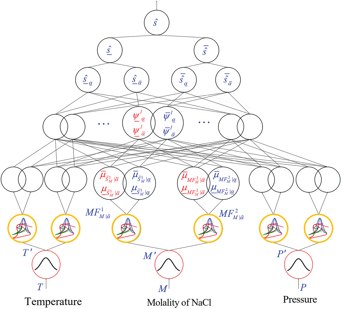
Figure 1: Flowchart of suggested T3-FLS

M′=exp⁡(−(M−χM)2σχM2) (1)

T′=exp⁡(−(T−χT)2σχT2), P′=exp⁡(−(P−χP)2σχP2) (2)

where, χM , χT and χP are the centers of type-1 MFs and σχM , σχP and σχT are the corresponding standard division. At each sample time t the centers χM , χT and χP are to be values of inputs M, T and P and the standard divisions σχM , σχP and σχT are considered to be fixed.

2)   Two type-3 membership functions (MFs) are considered for inputs T, P and M as MFT1−MFT2 , MFP1−MFP2 and MFM1−MFM2 respectively. The number of horizontal slices is considered to be n. The memberships are computed as follows (see Figs. 2 and 3).

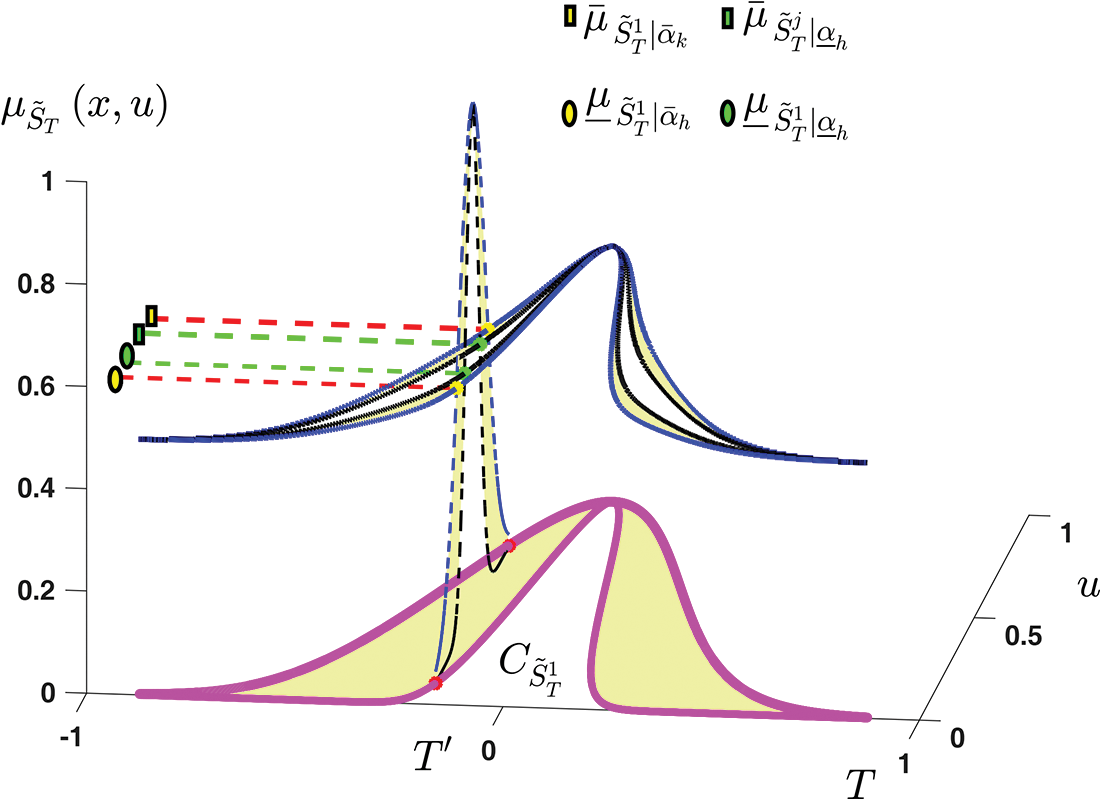
Figure 2: The horizontal slices of type-3 MF

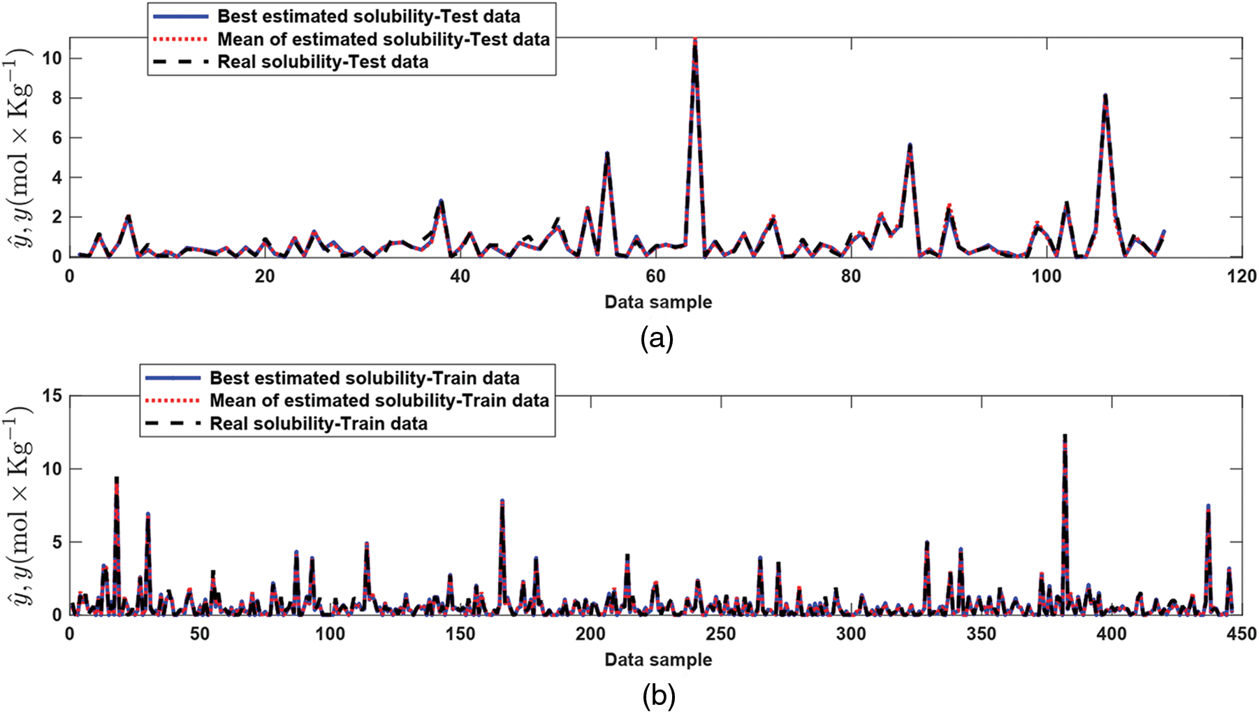
Figure 3: Estimation performance for Test data (a) and Training data (b)

μ¯MFTj|α¯h(T)=exp⁡(−(T¯α¯h−χMFTj|α¯h)2σ¯MFTj|α¯h2), μ¯MFTj|α_h(T)=exp⁡(−(T¯α_h−χMFTj|α_h)2σ¯MFTj|α_h2) (3)

μ_MFTj|α¯h(T)=exp⁡(−(T_α¯h−χMFTj|α¯h)2σ_MFTj|α¯h2), μ_MFTj|α_h(T)=exp⁡(−(T_α_h−χMFTj|α_h)2σ_MFTj|α_h2) (4)

where, χMFTj|α¯h and χMFTj|α_h are the centers of jth MF for input T, α_h and α¯h represent the h−th lower and upper horizontal slice. By using non-singleton fuzzification, T¯α¯h, T¯α_h, T_α¯h, T_α_h are obtained as:

T¯α¯h=σ¯MFTj|α¯h2T+σχT2χMFTj|α¯hσ¯MFTj|α¯h2+σχT2, T¯α_h=σ¯MFTj|α_h2T+σχT2χMFTj|α_hσ¯MFTj|α_h2+σχT2 (5)

T_α¯h=σ_MFTj|α¯h2T+σχT2χMFTj|α¯hσ_MFTj|α¯h2+σχT2, T_α_h=σ_MFTj|α_h2T+σχT2χMFTj|α_hσ_MFTj|α_h2+σχT2 (6)

Similarly For input P, one has:

μ¯MFPj|α¯h(P)=exp⁡(−(P¯α¯h−χMFPj|α¯h)2σ¯MFPj|α¯h2), μ¯MFPj|α_h(P)=exp⁡(−(P¯α_h−χMFPj|α_h)2σ¯MFPj|α_h2) (7)

μ_MFPj|α¯h(P)=exp⁡(−(P_α¯h−χMFPj|α¯h)2σ_MFPj|α¯h2), μ_MFPj|α_h(P)=exp⁡(−(P_α_h−χMFPj|α_h)2σ_MFPj|α_h2) (8)

where, χMFPj|α¯h and χMFPj|α_h are the centers of jth MF for input PP. The terms P¯α¯h , P¯α_h , P_α¯h and P_α_h are:

P¯α¯h=σ¯MFPj|α¯h2P+σχP2χMFPj|α¯hσ¯MFPj|α¯h2+σχP2, P¯α_h=σ¯MFPj|α_h2P+σχP2χMFPj|α_hσ¯MFPj|α_h2+σχP2 (9)

P_α¯h=σ_MFPj|α¯h2P+σχP2χMFPj|α¯hσ_MFPj|α¯h2+σχP2, P_α_h=σ_MFPj|α_h2P+σχP2χMFPj|α_hσ_MFPj|α_h2+σχP2 (10)

For input M, the relations are:

μ¯MFMj|α¯h(M)=exp⁡(−(M¯α¯h−χMFMj|α¯h)2σ¯MFMj|α¯h2), μ¯MFMj|α_h(M)=exp⁡(−(M¯α_h−χMFMj|α_h)2σ¯MFMj|α_h2)

μ_MFMj|α¯h(M)=exp⁡(−(M_α¯h−χMFMj|α¯h)2σ_MFMj|α¯h2), μ_MFMj|α_h(M)=exp⁡(−(M_α_h−χMFMj|α_h)2σ_MFMj|α_h2) (11)

where,

M¯α¯h=σ¯MFMj|α¯h2M+σχM2χMFMj|α¯hσ¯MFMj|α¯h2+σχM2, M¯α_h=σ¯MFMj|α_h2M+σχM2χMFMj|α_hσ¯MFMj|α_h2+σχM2 (12)

M_α¯h=σ_MFMj|α¯h2M+σχM2χMFMj|α¯hσ_MFMj|α¯h2+σχM2, M_α_h=σ_MFMj|α_h2M+σχM2χMFMj|α_hσ_MFMj|α_h2+σχM2 (13)

For better seen the computations of memberships, the Fig. 2 is presented. We see form Fig. 2, that in T3-FLS, at each point we have four memberships. Two of them represent the upper/lower bounds for the upper membership, and the two others denote the upper/lower bounds for the lower membership.

3)   The all-possible rules are considered. Since we have 4 memberships (2 for upper memberships and 2 for lower memberships), the rule firings also have 4 degrees. The rule firings at α¯h are obtained as:

ψ¯α¯h=μ¯MFTi|α¯hμ¯MFPj|α¯hμ¯MFMk|α¯h, ψ¯α_h=μ¯MFTi|α_hμ¯MFPj|α_hμ¯MFMk|α_hψ_α¯h=μ_MFTi|α¯hμ_MFPj|α¯hμ_MFMk|α¯h, ψ_α_h=μ_MFTi|α_hμ_MFPj|α_hμ_MFMk|α_h (14)

where, i, j, k=1, 2 .

3)   For the first type-reduction one has:

s^¯α¯h=∑l=1Rψ¯α¯hlθ¯l∑l=1R(ψ¯α¯hl+ψ_α¯hl), s^¯α_h=∑l=1Rψ¯α_hlθ¯l∑l=1R(ψ¯α_hl+ψ_α_hl), s^_α¯h=∑l=1Rψ_α¯hlθ_l∑l=1R(ψ¯α¯hl+ψ_α¯hl), s^_α_h=∑l=1Rψ¯α_hlθ_l∑l=1R(ψ_α_hl+ψ_α_hl) (15)

where, R represents the number of rules, θl and θ_l are l−th rule parameters.

4)    For the second type-reduction, it can be written:

s^¯=∑h=1nα¯hs^¯α¯h∑h=1n(α¯h+α_h)+∑h=1nα_hs^¯α_h∑h=1n(α¯h+α_h), s^_=∑h=1nα¯hs^_α¯h∑h=1n(α¯h+α_h)+∑h=1nα_hs^_α_h∑h=1n(α¯h+α_h) (16)

5)    Finally, the estimated solubility ( s^ mol ⋅ Kg−1) is obtained as:

s^=s^¯+s^_2 (17)

3  Learning Scheme

The tuning scheme of rules and MF parameters are explained in this part.

3.1 Tuning Scheme of Rules

The rules are optimized by the EKF algorithm. The vector of rule parameters θ¯ and θ are learned by the following cost function:

J=(sd−s^)2/2 (18)

where, sd is the reference signal and s^ is estimated solubility. The learning laws are obtained as:

θ¯(t)=θ¯(t−1)+ϕ¯(t)ξ¯(t)(sd−s^), θ_(t)=θ_(t−1)+ϕ_(t)ξ_(t)(sd−s^) (19)

where, ϕ¯ and ϕ(t) represent covariance matrices for θ¯ and, θ_ . ξ¯(t) and ξ_(t)

ξ¯=[ξ¯1, …, ξ¯l, …, ξ¯R]T, ξ_=[ξ_1, …, ξ_l, …, ξ_R]T (20)

where, ξ¯(t) and ξ_(t) are:

ξ¯l=∂s^∂θ¯l=∂s^∂s^¯∂s^¯∂θ¯l=∂s^∂s^¯∂s^¯∂s^¯α¯h∂s^¯α¯h∂θ¯l+∂s^∂s^¯∂s^¯∂s^¯α_h∂s^¯α_h∂θ¯l=1∑h=1n(α¯h+α_h)∑h=1nα¯hψ¯α¯hl∑l=1R(ψ¯α_hl+ψ_α_hl)+α_hψ¯α_hl∑l=1R(ψ¯α_hl+ψ_α_hl) (21)

ξ_l=∂s^∂θ_l=∂s^∂s^_∂s^_∂θ_l=∂s^∂s^_∂s^_∂s^_α¯h∂s^_α¯h∂θ_l+∂s^∂s^_∂s^_∂s^¯α_h∂s^_α_h∂θ_l=1∑h=1n(α¯h+α_h)∑h=1nα¯hψ_α¯hl∑l=1R(ψ¯α_hl+ψ_α_hl)+α_hψ_α_hl∑l=1R(ψ¯α_hl+ψ_α_hl) (22)

3.2 Optimizing of MF Parameters and Level of Horizontal Slices

The level of horizontal slices ( α_h and α¯h , h = 1,…, n) and the centers of

MFs ( χMFT1 , χMFT2 , χMFT2 , χMFT2 , χMFP1 and χMFP2 ) are tuned by the SCKF algorithm. The details are explained in below.

1-The state-space of NT3-FLS is rewritten as:

ζ(t+1)=ζ(t)+ν(t), s^(t+1)=NT3−FLS(x(t)|ζ(t))+υ(t) (23)

The covariance of ν (t) is shown by r and the covariance of υ (t) is denoted by q. u(t) and ζ (t) are:

x(t)=[M, T, P]T, ζ(t)=[χMFT1, χMFT2, χMFM1, χMFM2, χMFP1, χMFP2, α_1, …, α_n, α¯1, …, α¯n]T

2-Compute cubature points Ci, i = 1…, 2(6 + 2n) as:

Ci,t=ωt−1λi+ζt−1 (24)

where, ωt−1 is the error covariance at time t−1, 6 + 2n is the number of centers of inputs and number of horizontal slices. λi is defined as:

λi={6+2n[0⋯1i−thelement⋯0]T, i=1, …, 6+2n6+2n[0⋯−1i−thelement⋯0]T, i=6+2n+1, …, i=2(6+2n) (25)

3-For each cubature point in (25), evaluate the Eq. (23):

Zi(t)=NT3-FLS(x(t)|Ci,t), i=1, …, 2(6+2n) (26)

4-From (78), compute the mean of Z as Z¯ :

Z¯t=∑i=12(6+2n)Zi,t/[2(6+2n)] (27)

Define Πt−1 as:

Πt−1=12(6+2n)[Z1,t−1−Z¯t−1, …, Z2(6+2n),t−1−Z¯t−1]T (28)

5-From (80), the square-root of covariance matrix is obtained as:

Γzz,t−1=Tria([Πt−1δr,t−1]) (29)

6-The cross-covariance Πζz,t−1 is computed as:

Πζz,t−1=C¯t−1Πt−1T (30)

C¯t−1=12(6+2n)[C1,t−1−ζt−1, …, C2(6+2n),t−1−ζt−1]T (31)

7-Compute Kalman gain as:

Kt=(Πζz,t−1/Γzz,t−1T)/Γzz,t−1T (32)

8-Update the vector of trainable parameters ζ as:

ζt=ζt−1−Kt(st−Z¯t) (33)

9-Update error covariance as:

δr,t=Tria([ζt−1−KtΠt−1Ktδr,t−1]) (34)

4  Data Description

The real-word data set to evaluate the presented NT3-FLS are taken from [34–37]. The number of total data sets is 550, in which, 440 data sets are randomly selected for learning and remain 110 data sets are considered testing. The pressure data is between 0.98 and 1400 bar, molality is between 0.016 and 6.14 mol⋅Kg−1, the temperature is between 273.15 and 723.15 ◦K and solubility is between 0.01 and 12.35 mol ⋅ Kg−1.

5  Examination Indexes

To evaluate the suggested approach, the following indexes are used:

RMSE=1N∑t=1N(st−s^t)2, VAR=∑t=1N(st−s^t)2N−1 (35)

TIC=1N∑t=1N(st−s^t)21N∑t=1Nst2+1N∑t=1Ns^t2, R2=1−∑t=1N(st−s^t)2∑t=1N(1N∑t=1Nst−s^t)2 (36)

where, N is the number of data sets and st and s^t are the real and estimated solubility.

6  Simulation

The estimation capability of the designed NT3-FLS is examined in this section and is compared with some similar methods.

6.1 Testing Data

The performance for both test and training data is depicted in Fig. 3. From Fig. 3, we observe that the estimated signal reaches the measured solubility well. The supremum of the trajectory of absolute estimation error is less than 0.5 mol⋅Kg−1. The worst, best, and mean of TIC, VAR, RMSE, and R-squared for test data are shown in Fig. 4. The mean of RMSE, VAR, TIC, and R-squared is about 0.2, 0.03, 0.07, and 0.97, respectively. The values of TIC at iterations 1–10 are given in Fig. 5. The histogram plot shows that for half of the iterations, the value of TIC is about 0.07, and its dispersion is too small. From the box plot, it is seen that the mean of TIC is about 0.07. The values of RMSEs concerning the epochs and histogram-box plots of RMSEs are depicted in Figs. 6a–6c. The mean of RMSE for test data is about 0.2, and its dispersion in various iterations is too small. Similarly, the values of VAR with respect to the epochs, histogram, and box plots are depicted in Figs. 7a–7c. It is seen that the variance of the approximated signal is too small in various iterations. Finally, to show the robustness of the suggested estimation approach, the trajectory of R-squared in iterations 1–10, the histogram, and box plots are shown in Fig. 8. One can see that the mean of R-squared is too close to one that represents a well and strong proficiency with the desired reliability.

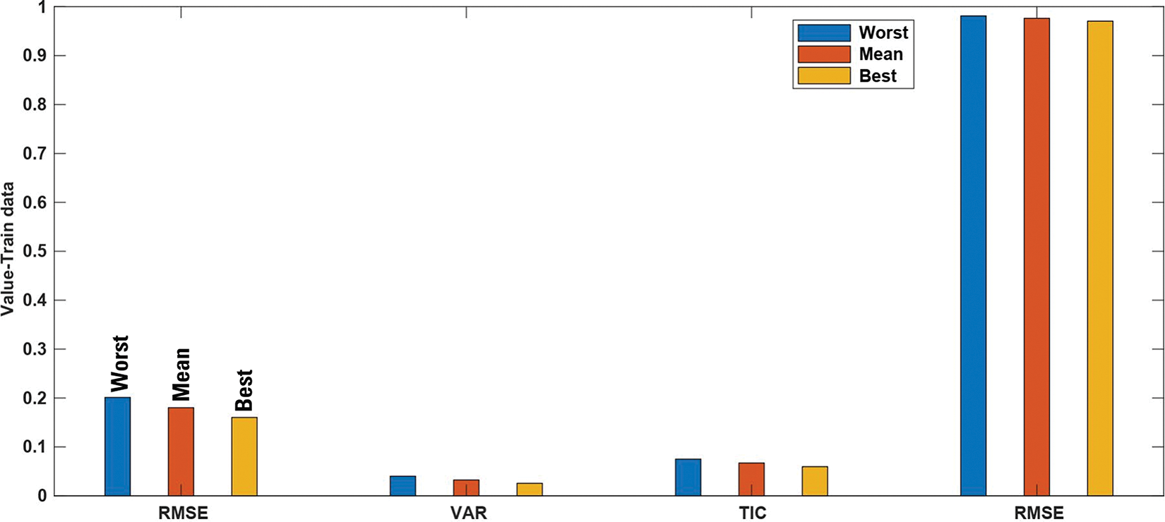
Figure 4: Testing data: RMSE, VAR, TIC and R-squared for

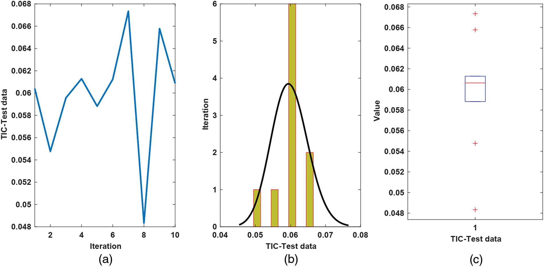
Figure 5: Results for TIC of test data, (a) The values of TIC; (b) Histogram; (c) Box plot

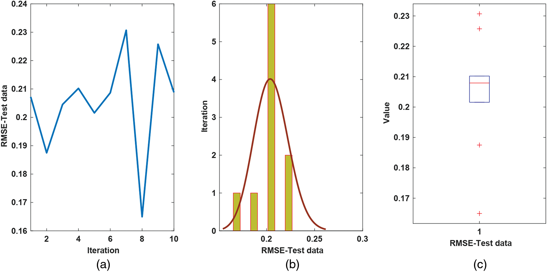
Figure 6: Results for RMSE of test data, (a) The value of RMSE; (b) Histogram plot; (c) Box plot

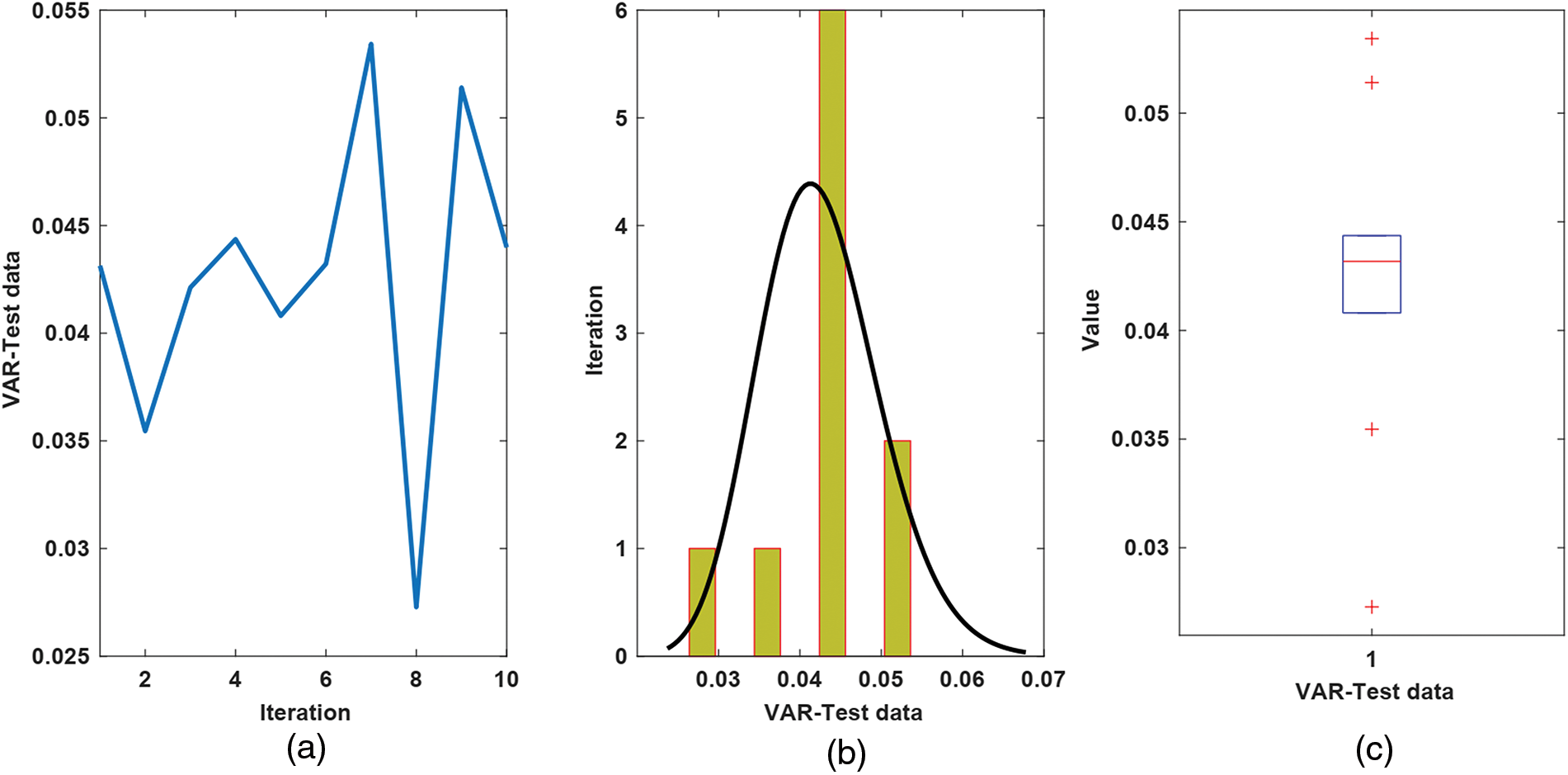
Figure 7: Results for VAR of test data, (a) The value of VAR; (b) Histogram plot; (c) Box plot

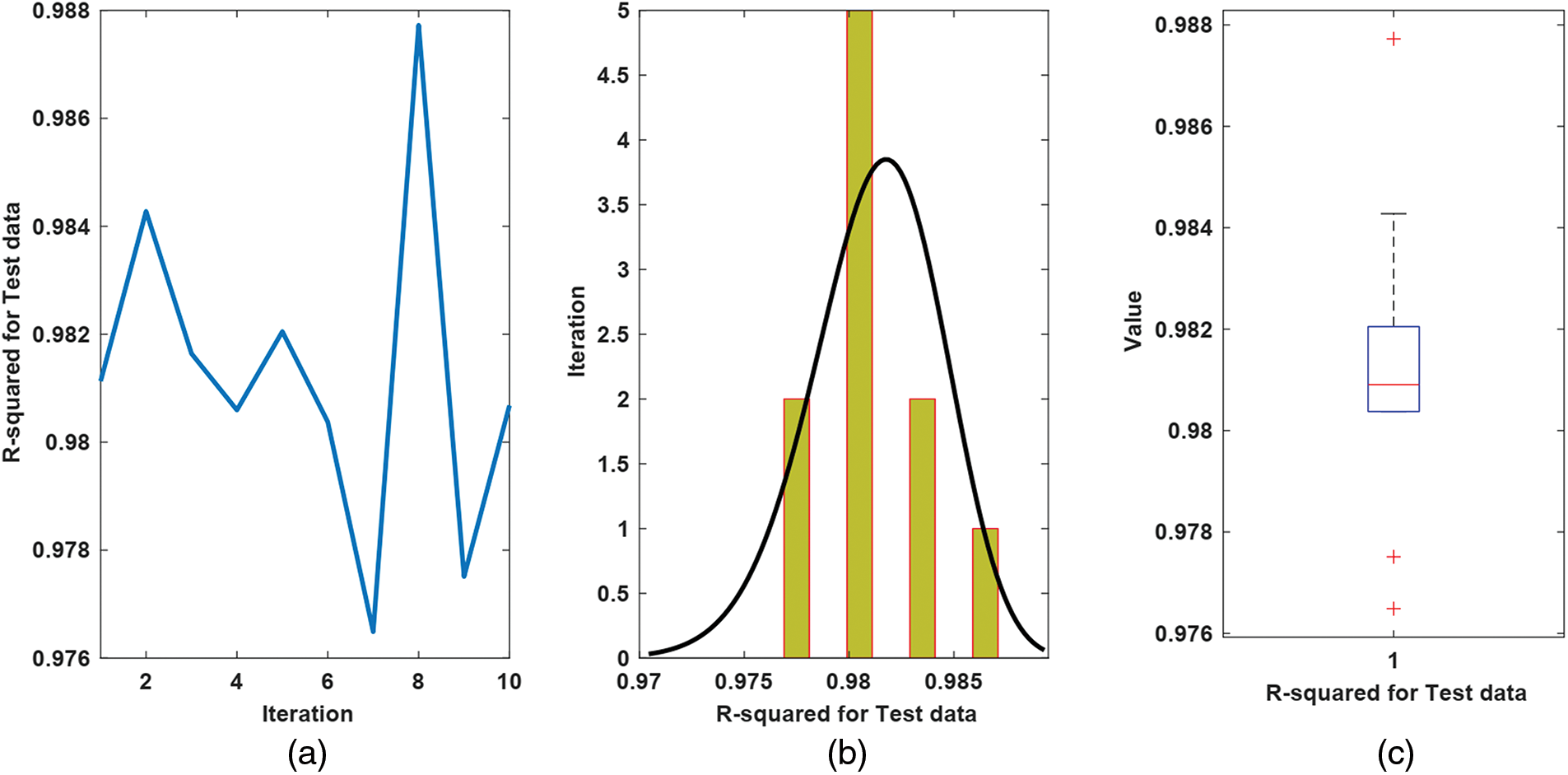
Figure 8: R2 analysis for test data, (a) The value of R2; plot. (b) Histogram plot; (c) Box

6.2 Comparison and Discussion

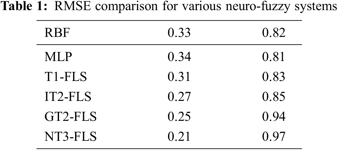
To better evacuate the suggested NT3-FLS, a comparison is given. The RMSE and R-squared are compared with radial-basis function NN (RBF-NN), type-1 FLS (T1-FLS), multi-layer-perceptron (MLP), interval type-2 FLS (IT2-FLS) and general type-2 FLS (GT2-FLS). The comparisons in Table 1 reveal the suggested NT3-FLS has better RMSE. Furthermore, the R-squared for our method is closer to one that indicates better reliability.

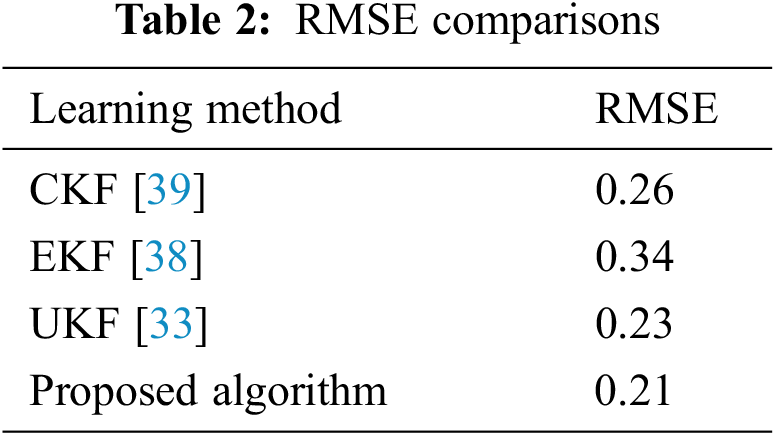
To further examine, a more comparison is presented with UKF [33], Extended Kalman filter (EKF) [38] and Cubature Kalman filter (CKF) [39] algorithms. The RMSEs are presented in Table 2, for different algorithms. One can observe that accuracy of the suggested learning technique is better than UKF, EKF, and CKF algorithms.

The proposed scheme can be developed by other fuzzy systems such as valued- T- spherical fuzzy approach [40], fuzzy linear programming [41], pythagorean fuzzy sets [42,43]. Also, the suggested approach can be used in various engineering applications such as control systems, signal processing, modeling problems, dynamic behavior analyzing, and so on [44–56].

7  Conclusion

In this study, the problem of CO2 capture and sequestration is studied, and a new machine learning approach is designed to forecast CO2 solubility in brine on basis of effective factors. The suggested method is designed by T3-FLSs and non-singleton fuzzification. The input measurement errors are modeled by a Gaussian MF. The optimization of the rule parameters is done by EKF, and the MF parameters and horizontal slice levels are tuned by SCKF. By a real-world data set the effectiveness of the suggested method is examined. It is shown that the mean of RMSE of the test data for 10 running times is less than 0.2 and also the mean of R-squared is more than 0.97 indicating a most reliable method. Also, by furthermore analysis such as investigating the values of TIC and VAR for several iterations, the fitness distribution is examined, and the good efficiency and accuracy of the suggested approach are shown. The accuracy of the suggested T3-FLS scheme is compared with some other FLSs such as RBF-NN, MLP, T1-FLS, IT2FLS, and GT2-FLS and other learning methods such as UKF, EKF, and CKF algorithms. The comparison results demonstrate the superiority of the designed technique on basis of NT3-FLS and the learning method using EKF and SCKF. For the future studies, the structure of NT3-FLS can also be trained, in addition to its parameters.

Funding Statement: This work was financially supported by the project of the National Social Science Fundation (21BJL052; 20BJY020; 20BJL127; 19BJY090); the 2018 Fujian Social Science Planning Project (FJ2018B067); The Planning Fund Project of Humanities and Social Sciences Research of the Ministry of Education in 2019 (19YJA790102), The grant has been received by Aoqi Xu.

Conflicts of Interest: The authors declare that they have no conflicts of interest to report regarding the present study.

References

1. C. Voyant, G. Notton, S. Kalogirou, M. -L. Nivet, C. Paoli, “Machine learning methods for solar radiation forecasting: A review,” Renewable Energy, vol. 105, pp. 569–582, 2017. [Google Scholar]

2. W. Arabameri, T. Chen, J. Blaschke, B. Tiefenbacher, B. Pradhan et al., “Gully head-cut distribution modeling using machine learning methods—a case study of nw Iran,” Water, vol. 12, no. 1, pp. 16, 2020. [Google Scholar]

3. S. Fathi, R. Srinivasan, A. Fenner and S. Fathi, “Machine learning applications in urban building energy performance forecasting: A systematic review,” Renewable and Sustainable Energy Reviews, vol. 133, pp. 110287, 2020. [Google Scholar]

4. R. L. Kumar, F. Khan, S. Din, S. S. Band, A. Mosavi et al., “Recurrent neural network and reinforcement learning model for covid19 prediction,” Frontiers in Public Health, vol. 9, 2021. [Online]. Available: https://doi.org/10.3389/fpubh.2021.744100 [Google Scholar] [PubMed] [CrossRef]

5. M. A. Ozdemir, O. K. Cura and A. Akan, “Epileptic eeg classification by using time-frequency images for deep learning,” International Journal of Neural Systems, vol. 31, no. 8, pp. 2150026, 2021. [Google Scholar] [PubMed]

6. C. K. Fisher, A. M. Smith and J. R. Walsh, “Machine learning for comprehensive forecasting of Alzheimer’s disease progression,” Scientific Reports, vol. 9, no. 1, pp. 1–14, 2019. [Google Scholar]

7. S. D. O. Domingos, J. F. de Oliveira and P. P. S. de Mattos Neto, “An intelligent hybridization of arima with machine learning models for time series forecasting,” Knowledge-Based Systems, vol. 175, pp. 72–86, 2019. [Google Scholar]

8. A. Khwaja, A. Anpalagan, M. Naeem and B. Venkatesh, “Joint baggedboosted artificial neural networks: Using ensemble machine learning to improve short-term electricity load forecasting,” Electric Power Systems Research, vol. 179, pp. 106080, 2020. [Google Scholar]

9. M. Hu, W. Li, K. Yan, Z. Ji and H. Hu, “Modern machine learning techniques for univariate tunnel settlement forecasting: A comparative study,” Mathematical Problems in Engineering, vol. 2019, 2019. [Online]. Available: https://doi.org/10.1155/2019/7057612 [Google Scholar] [CrossRef]

10. S. Sun, Y. Wei, K. -L. Tsui and S. Wang, “Forecasting tourist arrivals with machine learning and internet search index,” Tourism Management, vol. 70, pp. 1–10, 2019. [Google Scholar]

11. H. Shih and S. Rajendran, “Comparison of time series methods and machine learning algorithms for forecasting Taiwan blood services foundation’s blood supply,” Journal of Healthcare Engineering, vol. 2019, 2019. [Online]. Available: https://doi.org/10.1155/2019/6123745 [Google Scholar] [PubMed] [CrossRef]

12. Y. Peng, L. Cheng, Y. Jiang and S. Zhu, “Examining Bayesian network modeling in identification of dangerous driving behavior,” PLOS one, vol. 16, no. 8, pp. 0252484, 2021. [Google Scholar]

13. N. Zdarsky, S. Treue and M. Esghaei, “A deep learning-based approach to video-based eye tracking for human psychophysics,” Frontiers in Human Neuroscience, vol. 15, 2021. [Online]. Available: https://doi.org/10.3389/fnhum.2021.685830 [Google Scholar] [PubMed] [CrossRef]

14. M. Tian, S. Yan and X. Tian, “Discrete approximate iterative method for fuzzy investment portfolio based on transaction cost threshold constraint,” Open Physics, vol. 17, no. 1, pp. 41–47, 2019. [Google Scholar]

15. A. Mohammadzadeh and S. Rathinasamy, “Energy management in photovoltaic battery hybrid systems: A novel type-2 fuzzy control,” International Journal of Hydrogen Energy, vol. 45, no. 41, pp. 20970–20982, 2020. [Google Scholar]

16. E. Harirchian and T. Lahmer, “Developing a hierarchical type-2 fuzzy logic model to improve rapid evaluation of earthquake hazard safety of existing buildings,” Structures, vol. 28, pp. 1384–1399, 2020. [Google Scholar]

17. W. Peng, C. Li, G. Zhang and J. Yi, “Interval type-2 fuzzy logic-based transmission power allocation strategy for lifetime maximization of wsns,” Engineering Applications of Artificial Intelligence, vol. 87, pp. 103269, 2020. [Google Scholar]

18. E. Ontiveros, P. P. Melin and O. Castillo, “Comparative study of interval type-2 and general type-2 fuzzy systems in medical diagnosis,” Information Sciences, vol. 525, pp. 37–53, 2020. [Google Scholar]

19. P. P. K. Mishro, S. Agrawal, R. Panda and A. Abraham, “A novel type-2 fuzzy C-means clustering for brain mr image segmentation,” IEEE Transactions on Cybernetics, vol. 51, no. 8, pp. 3901–3912, 2021. [Google Scholar] [PubMed]

20. J. Li, Z. -M. Liu, C. Li and Z. Zheng, “Improved artificial immune system algorithm for type-2 fuzzy flexible job shop scheduling problem,” IEEE Transactions on Fuzzy Systems, vol. 29, no. 11, pp. 3234–3248, 2021. [Google Scholar]

21. A. M. Omer Abbaker, H. Wang, and Y. Tian, “Robust model-free adaptive interval type-2 fuzzy sliding mode control for PEMFC system using disturbance observer,” International Journal of Fuzzy Systems, vol. 22, no. 7, pp. 2188–2203, 2020. [Google Scholar]

22. T. Hosseinzadeh Khonakdari, and M. Ahmadi Kamarposhti, “Real-time detection of microgrid islanding considering sources of uncertainty using type-2 fuzzy logic and PSO algorithm,” PloS one, vol. 16, no. 9, pp.e 0257830, 2021. https://doi.org/10.1371/journal.pone.0259925 [Google Scholar] [PubMed] [CrossRef]

23. S. N. Qasem, A. Ahmadian, A. Mohammadzadeh, S. Rathinasamy, and B. Pahlevanzadeh, “A Type-3 logic fuzzy system: Optimized by a correntropy based kalman filter with adaptive fuzzy kernel size,” Information Sciences, vol. 572, pp. 424–443, 2021. [Google Scholar]

24. K. J. Coyne, L. R. Salvitti, A. M. Mangum, G. Ozbay, C. R. Main et al., “Interactive effects of light, CO2 and temperature on growth and resource partitioning by the mixotrophic dinoflagellate, karlodinium veneficum,” Plos one, vol. 16, no. 10, p.e 0259161, 2021. [Google Scholar]

25. H. S. Nogay, and H. Adeli, “Detection of epileptic seizure using pretrained deep convolutional neural network and transfer learning,” European Neurology, vol. 83, no. 6, pp. 602–614, 2020. [Google Scholar] [PubMed]

26. A. Bemani, A. Baghban, and A. Mosavi, “Estimating CO2-brine diffusivity using hybrid models of ANFIS and evolutionary algorithms,” Engineering Applications of Computational Fluid Mechanics, vol. 14, no. 1, pp. 818–834, 2020. [Google Scholar]

27. E. Mohammadian, S. Motamedi, S. Shamshirband, R. Hashim, R. Junin et al., “Application of extreme learning machine for prediction of aqueous solubility of carbon dioxide,” Environmental Earth Sciences, vol. 75, no. 3, pp. 1–11, 2016. [Google Scholar]

28. B. Shabani and J. Vilcáez, “Prediction of co2-ch4-h2s-n2 gas mixtures solubility in brine using a non-iterative fugacity-activity model relevant to co2-meor,” Journal of Petroleum Science and Engineering, vol. 150, pp. 162–179, 2017. [Google Scholar]

29. H. Chen, M. Zeng, H. Zhang, B. Chen, L. Guan et al., “Prediction of carbon dioxide solubility in polymers based on adaptive particle swarm optimization and least squares support vector machine,” ChemistrySelect, vol. 7, no. 3, p.e 202104447, 2022. [Google Scholar]

30. R. R. Ratnakar, A. Venkatraman, A. Kalra and B. Dindoruk, “On the prediction of gas solubility in brine solutions with single or mixed salts: Applications to gas injection and co2 capture/sequestration,” Journal of Natural Gas Science and Engineering, vol. 81, pp. 103450, 2020. [Google Scholar]

31. R. R. Ratnakar, A. Venkatraman, A. Kalra and B. Dindoruk, “On the prediction of gas solubility in brine solutions for applications of co2 capture and sequestration,” in SPE Annual Technical Conf. and Exhibition. Society of Petroleum Engineers, Dallas, Texas, USA, 2018. [Online]. Available: https://doi.org/10.2118/191541-MS [Google Scholar] [CrossRef]

32. A. Mohammadzadeh, M. H. Sabzalian and W. Zhang, “An interval type-3 fuzzy system and a new online fractional-order learning algorithm: Theory and practice,” IEEE Transactions on Fuzzy Systems, vol. 28, pp. 1940–1950, 2019. https://doi.org/10.1109/TFUZZ.2019.2928509 [Google Scholar] [CrossRef]

33. M. -W. Tian, A. Mohammadzadeh, J. Tavoosi, S. Mobayen, J. H. Asad et al., “A Deep-learned type-3 fuzzy system and its application in modeling problems,” Acta Polytechnica Hungarica, vol. 19, no. 2, pp. 151–172, 2022. [Google Scholar]

34. W. Yan, S. Huang and E. H. Stenby, “Measurement and modeling of co2 solubility in nacl brine and co2–saturated nacl brine density,” International Journal of Greenhouse Gas Control, vol. 5, no. 6, pp. 1460–1477, 2011. https://doi.org/10.1016/j.ijggc.2011.08.004 [Google Scholar] [CrossRef]

35. A. Yasunishi and F. Yoshida, “Solubility of carbon dioxide in aqueous electrolyte solutions,” Journal of Chemical and Engineering Data, vol. 24, no. 1, pp. 11–14, 1979. [Google Scholar]

36. Y. Liu, M. Hou, G. Yang and B. Han, “Solubility of co2 in aqueous solutions of nacl, kcl, cacl2 and their mixed salts at different temperatures and pressures,” The Journal of Supercritical Fluids, vol. 56, no. 2, pp. 125–129, 2011. https://doi.org/10.1016/j.supflu.2010.12.003 [Google Scholar] [CrossRef]

37. N. A. Menad, A. Hemmati-Sarapardeh, A. Varamesh and S. Shamshirband, “Predicting solubility of co2 in brine by advanced machine learning systems: Application to carbon capture and sequestration,” Journal of CO2 Utilization, vol. 33, pp. 83–95, 2019. [Google Scholar]

38. A. -I. Szedlak-Stinean, R. -E. Precup, E. M. Petriu, R. -C. Roman, E. -L. Hedrea et al., “Extended kalman filter and takagisugeno fuzzy observer for a strip winding system,” Expert Systems with Applications, vol. 208, pp. 118215, 2022. [Google Scholar]

39. X. Yang, S. Wang, W. Xu, J. Qiao, C. Yu et al., “A novel fuzzy adaptive cubature kalman filtering method for the state of charge and state of energy co-estimation of lithium-ion batteries,” Electrochimica Acta, vol. 415, pp. 140241, 2022. [Google Scholar]

40. H. Garg, K. Ullah, T. Mahmood, Z. Ali and H. Khalifa,“Multi- attribute decision-making g problems based on aggregation operators with complex interval valued-T-spherical fuzzy information,” MAEJO International Journal of Science and Technology, vol. 16, no. 1, pp. 51–65, 2022. [Google Scholar]

41. H. A. Khalifa and P. Kumar, “Interval-type fuzzy linear fractional programming problem in neutrosophic environment: A fuzzy mathematical programming approach,” Neutrosophic Sets and Systems, vol. 47, pp. 38–49, 2021. [Google Scholar]

42. Ur. A. Atique, M. Saeed, W. A. Afifi and H. A. Khalifa, “Decision making algorithmic techniques based on aggregation operations and similarity measures of possibility intuitionistic fuzzy hypersoft sets,” AIMS Mathematics, vol. 7, no. 3, pp. 3866–3895, 2021. [Google Scholar]

43. I. Siddique, R. M. Zulqarnain, A. Iampan, A. Alburaikan and H. A. Khalifa, “A Decision-making approach based on score matrix for pythagorean fuzzy soft set,” Computational Intelligence and Neuroscience (Special Issue: Artificial Intelligence and Machine Learning-Driven Decision-Making), vol. 2021, Article ID 5447422, 2021. [Google Scholar]

44. A. U. Rahman, M. Saeed, S. S. Alodhaibi and H. A. El-Wahed Khalifa, “Decision making algorithmic approaches based on parameterization of neutrosophic set under hypersoft set environment with fuzzy, intuitionistic fuzzy and neutrosophic settings,” Computer Modeling in Engineering& Sciences, vol. 128, no. 2, pp. 843–777, 2021. [Google Scholar]

45. D. Li, S. S. Ge and T. H. Lee, “Fixed-time-synchronized consensus control of multiagent systems,” IEEE Transactions on Control of Network Systems, vol. 8, no. 1, pp. 89–98. 2021. [Google Scholar]

46. R. Hao, Z. Lu, H. Ding and L. Chen, “A nonlinear vibration isolator supported on a flexible plate: Analysis and experiment,” Nonlinear Dynamics, vol. 108, no. 2, pp. 941–958. 2022. [Google Scholar]

47. W. Zheng, X. Liu and L. Yin, “Research on image classification method based on improved multi-scale relational network,” PeerJ Computer Science, 2021, [Online]. Available: https://doi.org/10.7717/peerj-cs.613 [Google Scholar] [PubMed] [CrossRef]

48. Z. Ma, W. Zheng, X. Chen and L. Yin, “Joint embedding VQA model based on dynamic word vector,” PeerJ Computer Science, 2021. [Online]. Available: https://doi.org/10.7717/peerj-cs.353 [Google Scholar] [PubMed] [CrossRef]

49. W. Zheng, L. Yin, X. Chen, Z. Ma, S. Liu et al., “Knowledge base graph embedding module design for visual question answering model,” Pattern Recognition, vol. 120, pp. 108153, 2021. https://doi.org/10.1016/j.patcog.2021.108153 [Google Scholar] [CrossRef]

50. Y. Du, B. Qin, C. Zhao, Y. Zhu, J. Cao et al., “A novel spatio-temporal synchronization method of roadside asynchronous MMW radar-camera for sensor fusion,” IEEE Transactions on Intelligent Transportation Systems, vol. 23, no. 11, pp. 1–12, 2021. [Online]. Available: https://doi.org/10.1109/TITS.2021.3119079 [Google Scholar] [CrossRef]

51. Y. Li, P. Che, C. Liu, D. Wu and Y. Du, “Cross-scene pavement distress detection by a novel transfer learning framework,” Computer-aided Civil and Infrastructure Engineering, vol. 36, no. 11, pp. 1398–1415, 2021. https://doi.org/10.1111/mice.12674 [Google Scholar] [CrossRef]

52. G. Zhou, S. Long, J. Xu, X. Zhou, B. Song et al., “Comparison analysis of five waveform decomposition algorithms for the airborne LiDAR echo signal,” IEEE Journal of Selected Topics in Applied Earth Observations and Remote Sensing, vol. 14, pp. 7869–7880. 2021. [Google Scholar]

53. G. Zhou, R. Zhang and S. Huang, “Generalized buffering algorithm,” IEEE Access, vol. 9, pp. 27140–27157, 2021. [Google Scholar]

54. K. Ma, X. Hu, Z. Yue, Y. Wang, J. Yang et al., “Voltage regulation with electric taxi based on dynamic game strategy,” IEEE Transactions on Vehicular Technology, vol. 71, no. 3, pp. 2413–2426, 2022. [Google Scholar]

55. K. Ma, Z. Li, P. Liu, J. Yang, Y. Geng et al., “Reliability-constrained throughput optimization of industrial wireless sensor networks with energy harvesting relay,” IEEE Internet of Things Journal, vol. 8, no. 17, pp. 13343–13354, 2021. [Google Scholar]

56. Y. Shen, N. Ding, H. -T. Zheng, Y. Li and M. Yang, “Modeling relation paths for knowledge graph completion,” IEEE Transactions on Knowledge and Data Engineering, vol. 33, no. 11, pp. 3607–3617, 2021. [Google Scholar]