CNN-LSTM: A Novel Hybrid Deep Neural Network Model for Brain Tumor Classification

1  Introduction

Diagnose brain tumors as soon as possible for the best chance of successful therapy. It’s crucial to recognize the tumor’s stage, pathological kind, and grade before deciding on a therapy method. Neuro-oncologists have benefited from CAD methods in a variety of ways. Tumor identification, categorization, and grading are all possible using CAD in neuro-oncology. The categorization of benign and malignant brain tumors using computer-aided design (CAD) is a hotly debated subject [1]. Glioma grading, a significant issue in cancer research [2], is another example of this. All of the aforementioned computer-aided design (CAD) technologies make use of brain MRI scans. Because MRI provides a greater contrast for brain soft tissues than computed tomography (CT) pictures, this is possible. Recently developed deep learning ideas in computer-aided medical diagnostics have enhanced performance. Medical image analysis of brain tumor research has widely utilized deep learning methods [3].

The earlier a brain tumor can be detected, the better the prognosis. The use of brain MRI in the diagnosis of individuals with brain tumors is critical. The ability of MRIs to give high-resolution information on brain structure and abnormality has a significant effect on medical image processing and analysis [4,5]. Neuroradiologist looks for tumors in brain images to see whether there are any abnormalities there. However, if a large amount of MRI data is being examined, there is a risk of incorrect categorization. Another reason for misdiagnosis is that human eyesight becomes less sensitive as the number of instances increases, especially when just a few slices are affected. It's also a lengthy process. As a result, an effective method for analyzing and classifying brain anomalies is required. An early diagnosis will enable the harm to be repaired and the appropriate therapy to be given to the patient as quickly as possible. For medical diagnosis, MRI scans are increasingly widely utilized in hospitals and clinics, particularly in brain imaging. With MRI, you can see details in soft tissues more clearly and it's painless. No ionizing radiation is used in MRI scans. Because it is non-radioactive, non-aggressive, and pain-free, MRI is often utilized in brain imaging.

Because of its efficient design and intricate connections without needing a large number of nodes, deep learning algorithms have recently established trends in object categorization [6]. Deep learning algorithms, particularly DLSTM, were used to classify brain MRI images as cancerous or benign in this study. The suggested approach makes use of augmentation methods including rotating, cropping, zooming, CLAHE equalization, and Random Rotation with panoramic stitching because of data constraints.

The rest of the paper is organized as follows; the proposed topic-related manuscript is analyzed in Section 2 and the proposed concept is explained in Section 3. In Section 4, experimental results are analyzed and the conclusion part is presented in Section 5.

2  Related Works

Many of the researchers had developed tumor classification using machine learning algorithms. Among them some of the works are analyzed here; According to Huang et al. [7], various data augmentation techniques are evaluated by using the most up-to-date deep learning modulation classifier. Modulated signals may be used to enhance the deep learning-based classifier using three different techniques: rotation, flip, and Gaussian noise. These methods can be used both during training and during classification. Calculations indicate that all three augmentation techniques increase classification accuracy. The rotation augmentation technique beats the flip method, both of which produce a better classification accuracy than the Gaussian noise method. An original 100% training dataset with no augmentation may achieve better classification accuracy with rotation and flip augmentation given just 12.5% of it.

Meta et al. [8] presented a classification model to optimize the productivity of categorizing floral pictures utilizing Deep CNN for feature extraction and other machine learning techniques for classification applications. After that, we showed how picture augmentation may help you do better on tests of skill. In the end, we examined the results of several machine-learning classifiers, such as the Support Vector Machine (SVM), Random Forest (RF), KNN, and Multi-Layer Perceptron (MLP). We used two datasets to test our categorization system: Oxford-17 Flowers and Oxford-102 Flowers. To create training and test datasets, we split each dataset in half. Using SVM Classifier, we were able to get an accuracy of 98.5% for the Oxford 102-Flowers Dataset. A 99.8% accuracy rate using MLP Classifier was obtained while using it to classify the Oxford 17-Flower Dataset.

Ramirez Rochacand et al. [9] investigates the effectiveness of such a technique on three deep learning classifiers: MLP, CNN, and LSTM. To begin, they use the original dataset to create a baseline. In the second step, they use principal component analysis to prepare the dataset for analysis (PCA). Third, they use PCA to clean up the dataset before using our Gaussian data augmentation (GDA) method to add more information to it. Based on the confusion matrix and classification report, we may evaluate performance by utilizing k-fold cross-validation and compiling our findings in numerical as well as visual form. All three classifiers performed better when used in conjunction with our PCA + GDA method, according to our tests.

A Fuzzy C-Mean (FCM) method was proposed by Saleck et al. [10] for determining a patient’s brain tumor mass. Through the use of pixel intensities, we were able to overcome the estimating problem of the number of clusters in the FCM. In this method, the texture feature extraction algorithm GLCM (Gray Level Co-Occurrence Matrix) is utilized to extract the features needed to estimate the threshold value. System sensitivity, specificity, and accuracy are analyzed to determine its overall performance.

Brain MRI characteristics were extracted using a transfer learning method by Deepak [11]. Meningioma, glioma, and pituitary tumors are the subject of this study, which uses a three-class categorization system. The input brain MRI characteristics are extracted using the GoogLeNet transfer learning model and then fed back into the model. SVM and KNN algorithms were used to classify the deep CNN feature that had been extracted. For 5-fold cross-validation, this method had a precision of 98 percent.

Sajjada et al. [12] demonstrated a deep-learning technique for categorizing multigrade brain tumors. Using a CNN model, the tumor is first segmented, and then different parameters are added to the segmented data to enhance the training samples before the model is trained using the pre-trained VGG-19 CNN model. These computations are 87.38% reliable with the raw data and 91.67% accurate with upgraded data.

Amin [13] used an image fusion technique to discriminate tumor- and non-tumor-bearing regions of the brain using MRI. MRI structural and texture data from the T1C, T1, and T2 MRI sequences are combined to look for brain tumors. Next, the combined data has been analyzed. Fusion uses the Daubechies wavelet kernel of the Discrete Wavelet Transform (DWT). When a fusion tumor is compared to a single sequence, the fusion process produces a more informative tumor. A partial differential diffusion filter (PDDF) is used to attenuate noise in the combined image. The brain MRI is segmented using the global thresholding method into the foreground (tumor) and background (non-tumor) areas.

In the above literature, the authors developed brain tumor classification using different algorithms with better output. Even though, some of the improvements are urgently needed for brain tumor classification. In [7], the accuracy of the classification system is to be improved. In [8], they used a limited number of images for the classification process. Moreover, some method needs improvement in time complexity and accuracy. To overcome the problems, in this paper efficient method is presented.

3  Proposed Tumour Classification Using Optimized LSTM Classifier

The proposed approach aims to effectively segment the tumor portion and classify a class of the tumor. To achieve this objective, hybrid CNN-LSTM is utilized. The overall structure of recommended technique is given in Fig. 1. The recommended technique involves four main steps namely, pre-processing, data augmentation, segmentation, and classification. In the beginning, the images are given to the pre-processing stage to remove the noise present in the image. Then, to increase the dataset quantity, the data augmentation process is used. For data augmentation, five operations are used Cropping, rotation, Zooming, contrast limited adaptive histogram equalization (CLAHE), and RRPS Algorithm. Then, the enhanced images are segmented using the APSO algorithm. After the segmentation, each segmented portion is given to the hybrid CNN-LSTM classifier to classify an image as normal. Finally, the performance of the proposed approach is evaluated. The proposed system architecture is given in Fig. 1.

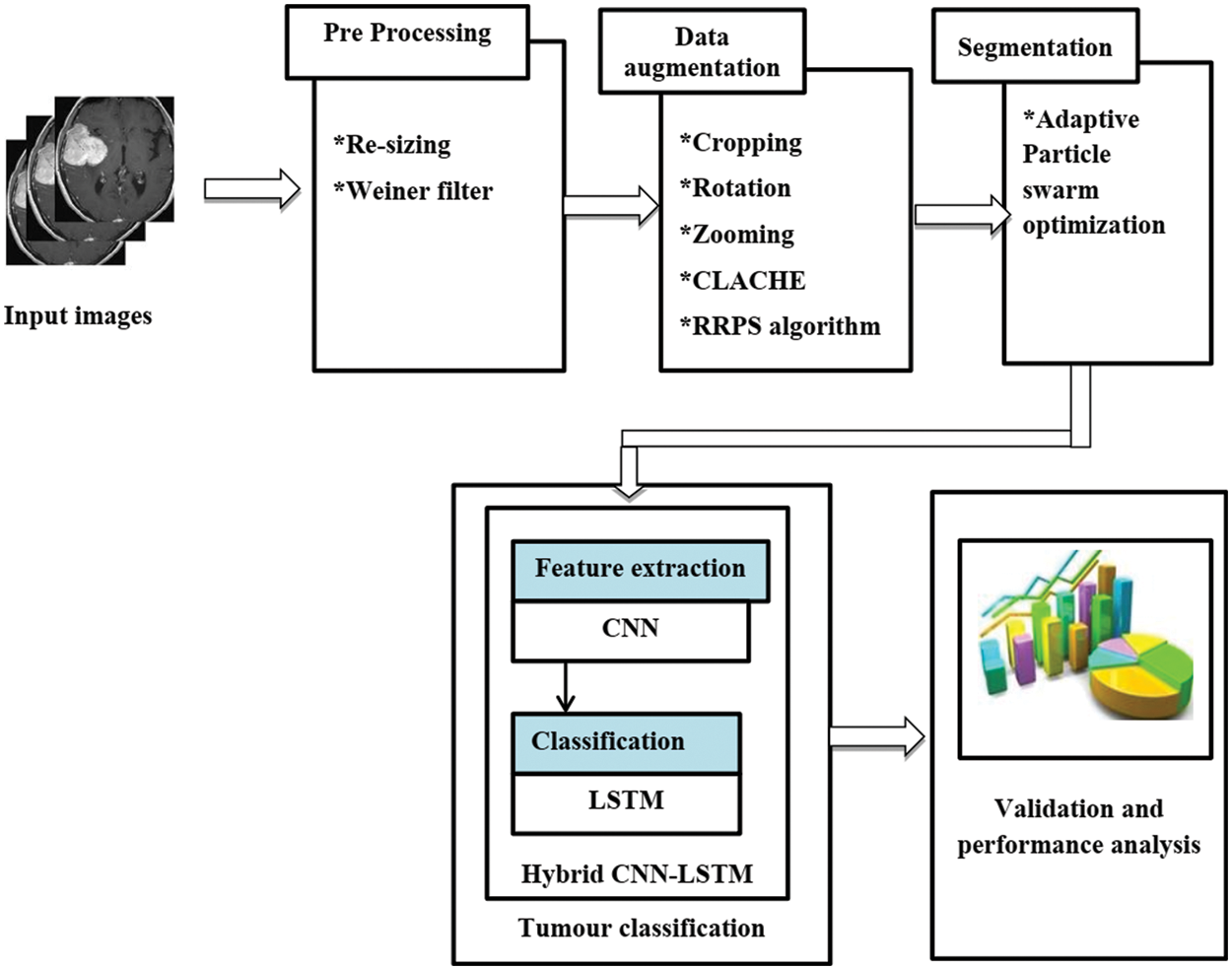
Figure 1: Proposed system architecture

3.1 Preprocessing

Patient data may be seen on the pictures in the database since they are unprocessed and noisy. Rician and salt-and-pepper noise dominate medical pictures [14]. The wiener filter works well with salt and pepper noise, as well as unipolar and bipolar impulse noise [15]. The wiener filter is employed in this technique to remove noise before the judgment step to obtain accuracy. One of the finest techniques for removing noise from MRI images is to use a wiener filter with a mask size of 7 * 7. Because patient movement causes distortions or noise in these pictures.

•   Image degradation due to additive noise and blur may be remedied using the MSE-optimal stationary linear Wiener filter.

•   To compute the Wiener filter, the signal and noise processes must be considered to be second-order stationery (in the random process sense).

•   The frequency domain is where Wiener filters are most often used. To get X from a deteriorated picture, one uses the DFT (Discrete Fourier Transform) (u,v). The Wiener filter G estimates the original picture spectrum by taking the product X(u,v) (u,v) [16]

S(u,v)=G(u,v)X(u,v)(1)

3.2 Data Augmentation

The amount of information in the dataset under consideration is very little. To achieve high accuracy, a classification model must be trained on a large volume of data. Images will be transformed into new kinds of data by changing size, zoom range, and theta. It creates new information from the old pictures by adjusting the angle, zoom, and flip. The model under consideration carries out the following five tasks:

•   Cropping

•   Rotation

•   Zoom

•   CLAHE equalization

•   Panorama stitching with random rotation

3.2.1 Cropping

The Centre patch of each frame may be cropped as a feasible processing step for image data that has a combination of height and width dimensions. You may also use random cropping in conjunction with translations to get the same results. With random cropping, smaller inputs will be produced, but with translations, the original image’s spatial dimensions are preserved. Let the upper-left corner’s coordinates serve as the origin, and the bottom-right corner’s coordinates serve as the end. (x, y) pixels in the new picture are equivalent to (x + origin.x, y + origin.y) pixels in the old image in terms of coordinates.

3.2.2 Rotation

Incorporating visual rotation in matching, alignment, and other image-based algorithms is quite ubiquitous. An image rotation method has three inputs: a picture, a rotation angle, and a rotation point. Rotation augmentations include turning the picture by 30 degrees either right or left. As previously mentioned, the rotation degree parameter significantly influences rotation augmentation safety. When a point’s coordinates (u1, v1) is rotated by an angle around (u0, v0), the new coordinates are (u2, v2) [11,12].

u2=cos⁡(θ)∗(u1−u0)+sin⁡(θ)∗(v1−v0)(2)

v2=sin⁡(θ)∗(u1−u0)+cos⁡(θ)∗(v1−v0)(3)

3.2.3 Zooming

Zooming simply means expanding a photograph such that the image’s fine features become more apparent and distinct. Zooming pictures requires the use of pixel replication. Narrowest neighbor interpolation is yet another name for it. This technique duplicates the pixels in the surrounding area, as the name suggests. By using this technique, new pixels are generated from the ones that have previously been provided. This technique duplicates each pixel n times, one in each row and column.

3.2.4 Contrast Limited Adaptive Histogram Equalization

As opposed to adaptive histogram equalization, contrast-restricted adaptive equalization is a more advanced version of it. It is a spatial domain contrast enhancement technique. It was first designed to improve the contrast in low-contrast medical pictures. In this method, pictures are divided into similar areas and equalization is found in every single region [16]. It flattens the distribution of grey levels, revealing more and more of the image’s previously hidden highlights as a result. It equalizes a picture to the greatest extent possible while also limiting the contrast. Because of the high brightness required, this method is very beneficial when used.

3.2.5 RRPS Algorithm

RRPS rotates the picture at random and either adds new pixel values around the image or interpolates existing pixel values, depending on the results. Then it stitches the original image with the reference image. The steps of the RRPS algorithm are given below;

•   The clip is revolved right or left by 1° to 359° on an axis used for rotation augmentations.

•   The rotation degree parameter has a substantial impact on the rotation augmentation.

•   Then the similarity of the original image with the adjacent reference image which is having at least 40% of overlap is calculated. Then the images are placed in the order from left to right.

•   Further SIFT features among images are generated.

•   Then the correspondence between features is established.

•   An initial estimate of Homography using inlier correspondence points is estimated to refine the Homography estimate using Levenberg–Marquardt optimization.

•   The above steps are repeated for each of the adjacent image pairs.

•   After obtaining Homographies for each of the picture pairs, get the demographics for the central image

•   All the images are projected using inverse warping.

3.3 Image Segmentation Using APSO Algorithm

After the data augmentation process, the images are given to the segmentation stage. For segmentation, in this paper, the APSO algorithm is utilized [17]. The APSO is a combination of PSO and oppositional-based learning (OBL) [18]. This OBL strategy avoids the local optimal of PSO and increases the searching ability. Using PSO-based methods for picture segmentation has been more common in the last decade. Using swarm intelligence, PSO is both a heuristic technique for global optimization and an optimization algorithm in and of itself. The idea of PSO was inspired by the behavior of swarms of particles and the social interactions that occur inside them. It’s like behavior for birds to become dispersed or to travel in groups in quest of food. As the birds migrate in search of food, the bird closest to it will be able to detect the scent of that food. There are n swarm particles in PSO, and the location of each particle represents a possible solution. The step-by-step process of APSO-based segmentation is explained below;

•   Keep its inertia

•   Improve the situation by relocating it to its ideal location.

•   Ensure that the swarm is at the best possible location by updating the condition.

Step 1: Solution Encoding: Solution encoding is a very crucial procedure for optimization. Initially, a user defines the number of clusters. Based on the number of clusters, the center points are randomly initialized. The center point is chosen in the X-axis value within the image width while the Y-axis value is within the image height. After the center point initialization, the parameters of PSO are also initialized.

Step 2: Opposite Solution Generation: After the solution initialization, to enhance the searching ability opposite solutions are generated.

Step 3: Fitness Calculation: After generating the initial solutions, the robustness of the solution is evaluated. The selection of fitness is a vital phase of the PSO algorithm. It is used to assess the ability (goodness) of solutions. The minimum distance is considered the objective function.

Step 4: Updation Using PSO: After the fitness calculation, the solutions are updated using the PSO operations. The velocity and positions of pixels are updated using Eqs. (4) and (5).

νidk+1=νidk+c1r1k(pbestidk−xidk)+c2r2k(gbestidk−xidk)(4)

xidk+1=xidk+νidk+1(5)

It is easy to see that in these two equations, each term represents a different quantity, such as the vkid and xkid denotes the speed of an individual particle at its most optimistic point in space and time pbestkid, and the location of that particle in space and time xbestkid. gbestkid represents the swarm’s optimistic d-dimension quantity. c 1 and c 2 represent the accelerating figures; they control the length while traveling to the most particle of the whole swarm and the most optimistic individual particle.

Step 5: Termination Criteria: The solutions are updated until attaining the optimal solution or best segmentation output. Once the solution is obtained, the algorithm will be terminated.

3.4 Classification Using Hybrid CNN-LSTM

After the segmentation process, the image is given to the input of a hybrid CNN-LSTM classifier. This classifier is a combination of individual CNN and LSTM classifiers. In this paper, for the training process, we set the learning rate as 0.005 with 1 = 0.9 and 2 = 0.999.

3.4.1 Convolution Neural Network

CNN is a multilayer perceptron utilized for some applications like image classification, object identification, and medical image classification. The fundamental thought behind a CNN is that it can get local features from high-layer inputs and move them to lower layers for additional complex features. A CNN comprises of convolution layer, a pooling layer, and a completely associated layer. The convolutional layer incorporates a bunch of kernels for deciding the tensor of component maps. These kernels connect the whole input utilizing “stride(s)” with the goal that the elements of a result block become numbers. The elements of the input block are diminished after the convolutional layer is utilized to execute the striding process.

M(i,j)=(Iin∗Ke)(i,j)=∑∑Iin(i+a,j+b)Ke(a,b)(6)

where; Iin represents the input matrix, Ke represents a 2D filter of size m×n, and F represents the output of a 2D feature map. In this paper, rectified linear unit (ReLU) layer is used to maximize the non-linearity feature map. The mathematical expression of the ReLU function is given in Eq. (7).

f(x)=max(0.x)(7)

The pooling layer is used to reduce the number of parameters and the fully connected layer performs the classification process.

3.4.2 LSTM Network

The LSTM is a sort of artificial neural network. Traditional neural networks don't think about consecutive factors. Additionally can’t survey past substances. To fathom this issue, the RNN is proposed. In this idea, the hidden state Ht is taken the input At from the input state and produces the result Lt-1. This approach is primarily utilized for present model loss capability and assess the following layer yield Lt + 1. Essentially RNN has criticism circles in a ceaseless layer. This licenses information to be taken care of in ‘memory’ long term. Nonetheless, it is hard to prepare standard RNNs to settle an issue that requires learning long-haul fleeting conditions. This is because the slant of the misfortune cycle diminishes dramatically with time. To avoid the problem, an efficient LSTM is proposed, which can fix long-distance reliability.

Lt=tan⁡L[wL(At,Lt−1)+cL](8)

where the hidden state control parameter is represented as cL, the weight parameter is denoted as wL, the input is represented as input AT and the tanL is utilized to add or remove data to the earlier input. the structure of LSTM is given in Fig. 2. The LSTM consists of forget gate, input gate, output gate, and TanL layer.

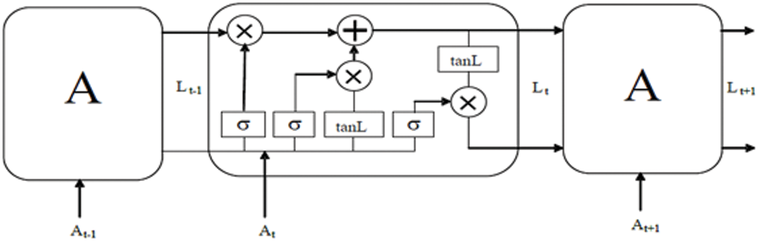
Figure 2: Architecture of LSTM

The forget gate is calculated using Eq. (9)

Ft=σ⌊WeiF(At,Lt−1)+cF⌋(9)

where, forget gate is represented as Ft, the control parameter of the forgetting gate is represented as CF, the weight of forget gate is represented as WeiF, the existing LSTM block output is represented as Lt-1 and the logistic sigmoid function is represented as σ. For the situation, the output accomplished is the ‘0’ signifies gates are blocked. If the result is ‘1’ gates permit all to go through. The input gate function is given in Eq. (10).

It=σ⌊WeiI(At,Lt−1)+cI⌋(10)

where, the input gate is representing It, LSTM block present output is represented as At, the weight present in the input gate is WeiI and the bias value of the input gate is represented as CI. The candidate value of tanL layer is calculated using Eq. (9) as follows;

Vt=tan⁡L⌊WeiV(At,Lt−1)+cV⌋(11)

where Vt represent the timestamp (t) for the cell state. tanL layer informs the network about weather information to be added or removed. The control parameter is Cv and Wv denotes the weight parameter. The output gate is calculated using Eq. (12).

Ot=σ⌊WeiO(At,Lt−1)+cO⌋(12)

where, the output gate is denoted a Ot, wo denote the weight value of the output neuron, and the bias value is denoted as Co. The output function is calculated using Eq. (13).

Lt=Ot∗tan⁡L(Vt)(13)

where, the * denotes the vector’s element-wise multiplication and the memory cell state is represented as Vt. Ht indicated the output of the current block. The total loss function of the LSTM system is given in Eq. (14).

Loss=∑t=1N(Lt−Tt)2(14)

where Tt is denoted as desired output and N represent the total number of data point to calculate the loss mean square error.

3.4.3 Hybrid CNN-LSTM

The proposed hybrid CNN-LSTM classifier is used to classify a given image as a normal or tumor image. The structure of the hybrid CNN-LSTM-based classification is given in Fig. 3.

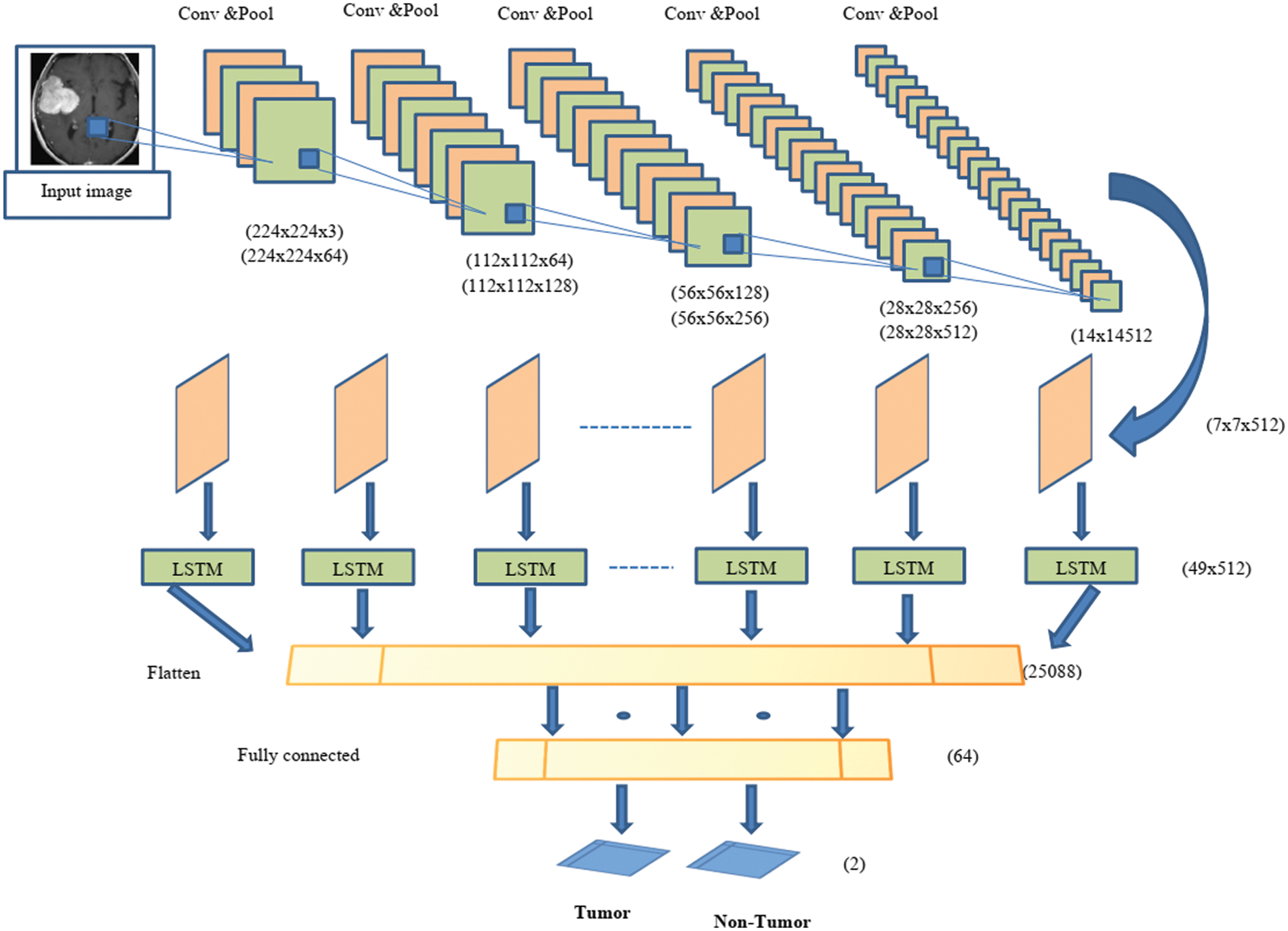
Figure 3: Structure of proposed hybrid CNN-LSTM

In this paper, a hybrid for automatic detection of tumor and non-tumor images is presented. CNN is used to extract features from the image and LSTM is used for the classification process. The proposed hybrid system consists of 20 layers, including 12 convolution layers, five pooling layers, a fully connected layer, an LSTM layer, and an output layer. Each convolution layer consists of two or three 2D CNNs and a pooling layer followed by a dropout layer. The convolution layer used a 3 × 3 kernel and ReLu activation function. A maximum-pooling layer with size 2 × 2 kernels is used to reduce the dimensions of the input image. In the last part of the architecture, the functional graph is transferred to the LSTM layer to extract the timing information. After the convolutional block, the output format is found to be (none, 7, 7, 512). Using the reconstruction method, the input size of the LSTM layer is (49, 512). After analyzing the time characteristics, the architecture sorts the X-ray images by fully connected layers, which are divided into two categories (normal image or tumor image).

4  Results and Discussion

The experimental results of the proposed tumor classification are presented in this section. The proposed approach is implemented using MATLAB with windows 10 and 4 GB RAM. The performance of the proposed approach is analyzed based on different metrics. For experimental analysis images were collected from the UCI Machinery laboratory. The image’ test results are shown in Fig. 4. Fig. 4a depicts the original image, whereas Fig. 4b depicts the filtered version of the primitive image. The rotated image is exposed in Fig. 4c, while the cropped image is shown in Fig. 4d. Figs. 4e and 4f depict a zoomed-in picture and a segmented image. The Wiener filter is used to expel any distortion and noise from the primary picture. With the optimal pixel count, this image seems perfectly obvious. MATLAB is used throughout the whole brain tumor categorization procedure. A confusion matrix is presented in Fig. 5.

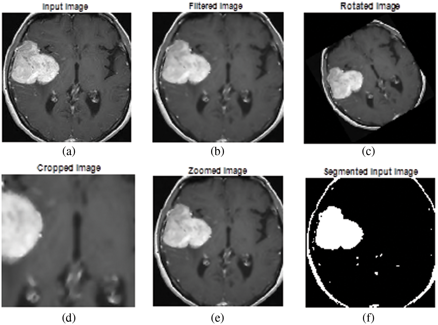
Figure 4: Experimental results (a) primary image, (b) filtered image, (c) rotated image, (d) cropped image, (e) zoomed image, and (f) segmented output

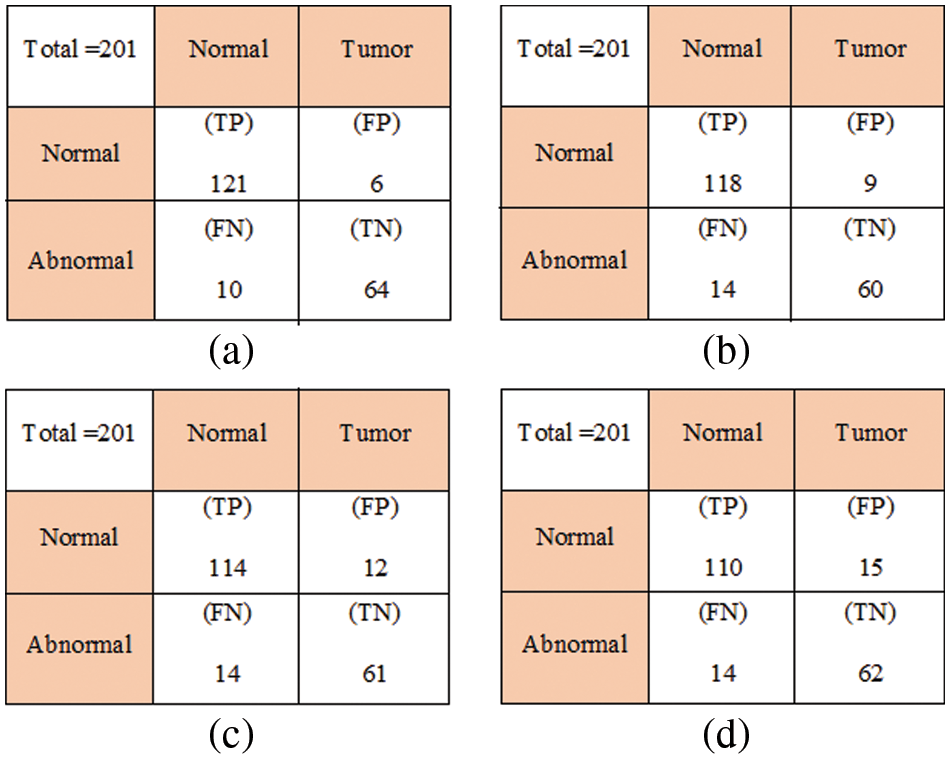
Figure 5: Confusion matrix (a) Hybrid CNN-LSTM, (b) LSTM, (c) SVM, and (d) ANN

4.1 Evaluation Metrics

Hybrid CNN-LSTM performance is obtained by counting the number of correct predictions of healthy and tumor images. To evaluate the quality of each designed architecture, the following performance metrics were used: accuracy, precision, recall, and specificity. These metrics are shown in the Table 1.

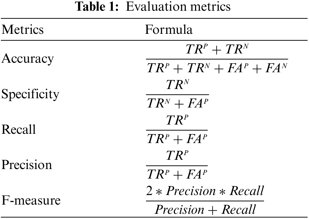
where; TRP, TRN, FAN, and FAP denote true positive, true negative, false negative, and false positive, respectively.

4.2 Comparative Analysis

To demonstrate the effectiveness of our recommended approach, we compare our work with various classifiers such as Support Vector Machine (SVM) [19], Artificial Neural Networks (ANN) [20], LSTM [21], and hybrid CNN-LSTM.

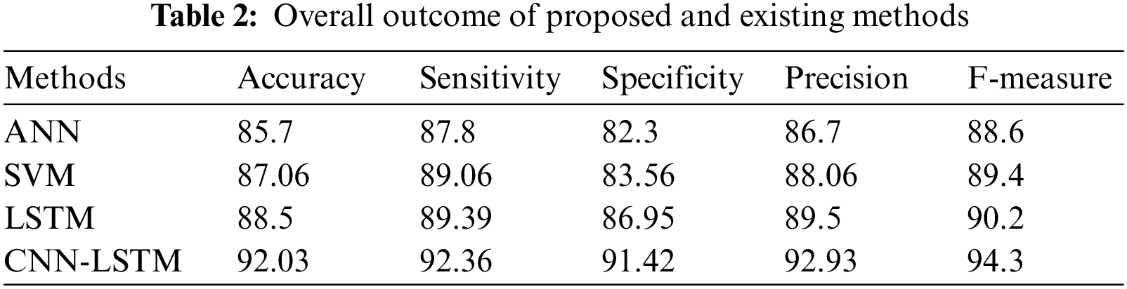
In Fig. 6, the effectiveness of the recommended approach is discussed based on accuracy. A good classification system should have maximum accuracy. In Fig. 6, we compare the effectiveness of the recommended approach with the different methods ANN, SVM, and LSTM. When analyzing Fig. 6, the recommended approach reached a maximum accuracy of 92.03%, which is 88.5% for the LSTM-based classification, 87.06% for the SVM-based classification, and 85.7% for the ANN-based classification. This is due to the hybridization of CNN and LSTM. Similarly, in Fig. 7, the efficiency of the recommended approach is depicted based on the recall measurement. When analyzing Fig. 7, the recommended approach attained a maximum recall of 92.36%, which is 3.32% better than the LSTM-based classification, 3.7% better than the SVM-based classification, and 5.19% better than the ANN-based classification. In Fig. 8, the efficiency of the recommended approach is analyzed based on the specification. Again, the recommended approach achieved better results compared to the existing methods. In Fig. 9, the efficiency of the recommended approach is analyzed based on an accurate measurement. When analyzing Fig. 9, our proposed approach reached a maximum accuracy of 92.93%, which is high compared to other methods. Similarly, our proposed approach reached the maximum F-measure compared to other methods which is shown in Fig. 10. The overall results of the proposed and existing approach are presented in Table 2. It is clear from the results that the proposed approach achieved better results compared to other methods.

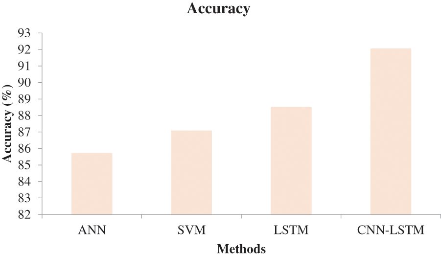
Figure 6: Comparative analysis based on accuracy

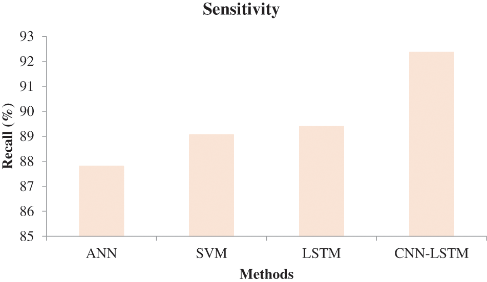
Figure 7: Comparative analysis based on sensitivity

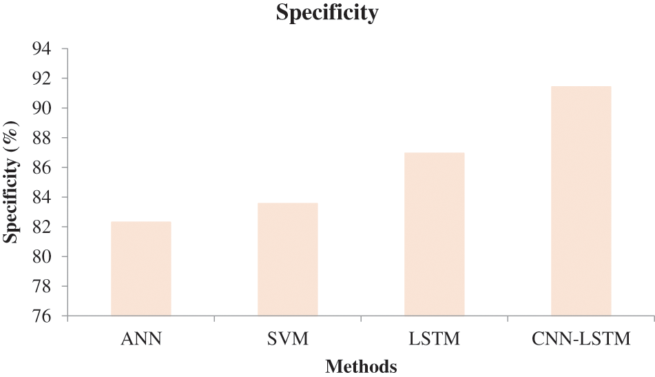
Figure 8: Comparative analysis based on specificity

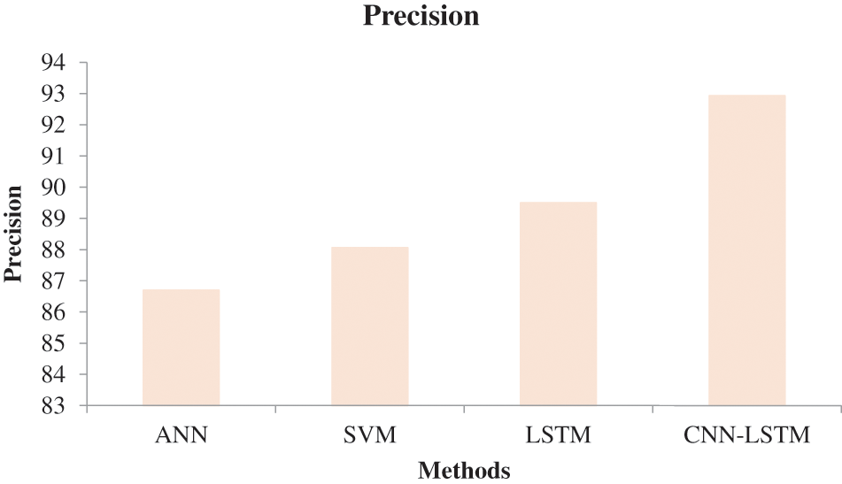
Figure 9: Comparative analysis based on precision

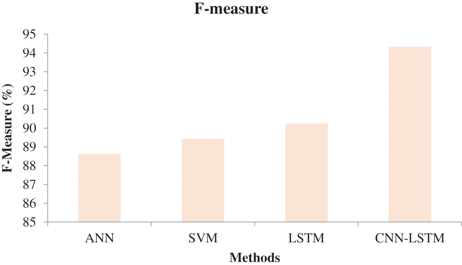
Figure 10: Comparative analysis based on F-measure

5  Conclusion

This report outlines a precise and completely automated method for the categorization of brain tumors that requires very little pre-processing. To extract characteristics from MRI scans, the suggested system made use of deep transfer learning. To enhance the prediction rate, more pictures are added using data augmentation methods. More fresh examples may be generated by utilizing label-maintained modifications and a picture superimposition method for data augmentation. To capture the most essential information, superimposed augmented pictures over the matching original images are utilized for training in this study, the hybrid CNN-LSTM classification model applies them. A novel Random rotation with a panoramic stitching method is presented using current data augmentation techniques such as rotation, cropping, and zooming. The proposed approach attained a maximum accuracy of 92.03%.

Acknowledgement: The author with a deep sense of gratitude would thank the supervisor for his guidance and constant support rendered during this research.

Funding Statement: The authors received no specific funding for this study.

Conflicts of Interest: : The authors declare that they have no conflicts of interest to report regarding the present study.

References

1. S. Kumar, C. Dabas and S. Godara, “Classification of brain MRI tumor images: A hybrid approach,” Procedia Computer Science, vol. 122, no. 9, pp. 510–517, 2017. https://doi.org/10.1016/j.procs.2017.11.400 [Google Scholar] [CrossRef]

2. G. Mohan and M. M. Subashini, “MRI based medical image analysis: Survey on brain tumor grade classification,” Biomedical Signal Processing and Control, vol. 39, pp. 139–161, 2019. https://doi.org/10.1016/j.bspc.2017.07.007 [Google Scholar] [CrossRef]

3. M. Talo, U. B. Baloglu and U. R. Acharya, “Application of deep transfer learning for automated brain abnormality classification using MR images,” Cognitive Systems Research, vol. 54, no. C, pp. 176–188, 2019. https://doi.org/10.1016/j.cogsys.2018.12.007 [Google Scholar] [CrossRef]

4. G. Litjens, “A survey on deep learning in medical image analysis,” Journal of Medical Image Analysis, vol. 42, no. 13, pp. 60–88, 2017. https://doi.org/10.1016/j.media.2017.07.005 [Google Scholar] [PubMed] [CrossRef]

5. L. Singh, “A novel machine learning approach for detecting the brain abnormalities from MRI structural images,” in Proc. of IAPR Int. Conf. on Pattern Recognition in Bioinformatics, Berlin Heidelberg, Springer, pp. 94–105, 2012. [Google Scholar]

6. D. Ravi, “Deep learning for health informatics,” IEEE Journal of Biomedical and Health Informatics, vol. 21, no. 1, pp. 4–21, 2017. https://doi.org/10.1109/JBHI.2016.2636665 [Google Scholar] [PubMed] [CrossRef]

7. L. Huang, W. Pan, Y. Zhang, L. Qian, N. Gao et al., “Data augmentation for deep learning-based radio modulation classification,” IEEE Access, vol. 8, pp. 1498–1506, 2020. https://doi.org/10.1109/ACCESS.2019.2960775 [Google Scholar] [CrossRef]

8. B. R. Mete and T. Ensari, “Flower classification with deep CNN and machine learning algorithms,” in Proc. of Int. Symp. on Multidisciplinary Studies and Innovative Technologies (ISMSIT), Turkey, 2019. [Google Scholar]

9. J. F. Ramirez Rochacand, L. Liang, N. Zhang and T. Oladunni, “A gaussian data augmentation technique on highly dimensional, limited labeled data for multiclass classification using deep learning,” in Proc. of Int. Conf. on Intelligent Control and Information Processing, Marrakesh, Morocco, pp. 14–19, 2019. [Google Scholar]

10. M. Saleck, “Tumor detection in mammography images using fuzzy C-means and GLCM texture features,” in Int. Conf. on Computer Graphics, Imaging and Visualization, Marrakesh, pp. 122–125, 2017. [Google Scholar]

11. S. Deepak, “Brain tumor classification using deep CNN features via transfer learning,” Journal of Computers in Biology and Medicine, vol. 111, no. 3, pp. 1–7, 2019. https://doi.org/10.1016/j.compbiomed.2019.103345 [Google Scholar] [PubMed] [CrossRef]

12. M. Sajjada, S. Khanb, K. Muhammad, W. Wu, A. U. Sung et al., “Multi-grade brain tumor classification using deep CNN with extensive data augmentation,” Journal of Computational Science, vol. 30, pp. 174–182, 2018. [Google Scholar]

13. J. Amin, “Brain tumor classification based on DWT fusion of MRI sequences using convolutional neural network,” Pattern Recognition Letters, vol. 129, pp. 115–122, 2020. https://doi.org/10.1016/j.patrec.2019.11.016 [Google Scholar] [CrossRef]

14. V. Wasule, “Classification of brain MRI using SVM and KNN classifier,” in Third Int. Conf. on Sensing, Signal Processing and Security (ICSSS), Chennai, pp. 218–223, 2017. [Google Scholar]

15. L. Cadena, “Noise reduction techniques for processing of medical images,” in Proc. of the World Congress on Engineering, London, pp. 4–9, 2017. [Google Scholar]

16. B. B. Singh and S. Patel, “Efficient medical image enhancement using CLAHE enhancement and wavelet fusion,” International Journal of Computer Applications, vol. 167, no. 5, pp. 1–5, 2017. [Google Scholar]

17. R. Poli, J. Kennedy and T. Blackwell, “Particle swarm optimization,” Swarm Intelligence, vol. 1, no. 1, pp. 33–57, 2017. [Google Scholar]

18. H. Wang, Z. Wu, S. Rahnamayan, Y. Liu and M. Ventresca, “Enhancing particle swarm optimization using generalized opposition-based learning,” Information Sciences, vol. 181, no. 20, pp. 4699–4714, 2011. https://doi.org/10.1016/j.ins.2011.03.016 [Google Scholar] [CrossRef]

19. N. Abdullah, U. K. Ngah and S. A. Aziz, “Image classification of brain MRI using support vector machine,” in The Proc. of the IEEE Int. Conf. on Imaging Systems and Techniques, Malaysia, pp. 242–247, 2011. [Google Scholar]

20. Y. Mohan, S. S. Chee, D. K. P. Xin and L. P. Foong, “Artificial neural network for classification of depressive and normal in EEG,” in 2016 IEEE EMBS Conf. on Biomedical Engineering and Sciences (IECBES), Malaysia, pp. 286–290, 2016. [Google Scholar]

21. S. Zhang, D. Zheng, X. Hu and M. Yang, “Bidirectional long short-term memory networks for relation classification,” in Proc. of the 29th Pacific Asia Conf. on Language, Information and Computation, China, pp. 73–78, 2015. [Google Scholar]