Energy Efficient Hyperparameter Tuned Deep Neural Network to Improve Accuracy of Near-Threshold Processor

1  Introduction

Their use for real-time inference on sensor-rich platforms such as the Internet of Things (IoT), wearables, personal biomedical devices, and drones is hampered by the energy and latency costs of existing machine learning (ML) approaches [1]. These applications [2] include devices that collect and analyse data to provide interpretations and actions that may be used to automate or monitor a variety of activities without human intervention. These types of methods must be able to include computationally intensive machine learning techniques while adhering to severe limitations on form factor, energy, and latency [3]. Memory access is known to reduce both the latency and the energy cost associated with machine learning algorithm comprehension. In recent years, several machine learning systems that utilise energy-efficient digital architectures and integrated circuits (IC) have been created. These applications employ methods like as efficient data flow, data reuse, and the optimization of computations to reduce the amount of memory accesses [4].

In order to conserve the needed amount of energy, the authors have reached a consensus on using this complete technique. This is owing to the stringent energy restrictions put on them. This technique covers every component of a computer system, from hardware to software [5]. Near-exact computing, also known as approximation computing, is one of the most cost-effective ways to preserve energy. This type of computing is sometimes referred to as “approximate computing.” This technology sacrifices application precision in order to reduce energy consumption. The assumption that certain applications, but not many, required the level of accuracy afforded by programming methods or current circuits was the impetus for the invention of this technology [6]. As an illustration, video decryption can tolerate a substantial amount of mistake since image variations cannot be seen by the human eye. This enables the utilisation of video decryption. It is anticipated that multicore architectures (embedding and increased performance) would rely largely on accelerators for many computationally intensive tasks (heterogeneous multicores). This is because the lack of voltage scaling leads to a phenomenon known as Dark Silicon. This architectural trend was motivated by the increasing limits put on accessible energy. Beyond typical accelerator solutions such as Application Specific Integrated Circuits (ASICs), Graphics Processing Units (GPUs), and Field Programmable Gate Arrays (FPGAs), writers are studying co-processors or accelerators with an intermediate scope in terms of generality. These co-processors or accelerators contain more applications than ASICs but less than general-purpose processors. In compared to FPGAs and GPUs, this is done in order to maximise energy efficiency. In particular, the authors [7] Coprocessors and accelerators whose capabilities fall somewhere in the centre. The present practise of integrating many accelerators into a single chip may lead the combined application scopes of these accelerators to encompass a vast amount of territory. This development is a result of the present practice of incorporating many accelerators on a chip. The second observed trend may be attributable to applications that are getting more computationally intensive.

Deep neural networks (DNNs) have demonstrated exceptional performance in cognitive tasks such as image and speech recognition [8]. This achievement has transformed the field of artificial intelligence (AI), and DNNs are also known as DNNs. Edge computing applications have a great interest in discovering platforms that could deploy the well-trained approach of these networks and perform inference in an energy-efficient manner. Specifically, battery-powered Internet of Things devices and autonomous vehicles benefited greatly from the speed, energy economy, and reliability of DNN’s inference engines [9]. [Bibliography required] With the development of specialised hardware for inference that runs at reduced digital precision (four to eight bits), such as low-power graphics processing units and Google’s tensor processing unit1 like NVIDIA T42, significant progress was achieved in this field. This was a significant advance in the correct direction. These are a few examples of something known as a low-power graphics processing unit. Even while such platforms have the potential to be extremely flexible, they nonetheless require a framework in which the processor and memory units are physically separated [10]. Even if such platforms have the potential to be very adaptable, they still require such a framework. There was a continuous flow of data between the memory and the processors since the procedures were typically kept in off-chip memory. This resulted in frequent memory access and modification. As a result, the maximum level of energy efficiency that could be achieved with the available resources reduced. In this study, an Energy Efficient Hyperparameter Tuned Deep Neural Network (EEHPT-DNN) model for Variation-Tolerant Near-Threshold Processor was developed. In order to improve the energy efficiency of artificial intelligence (AI), the EEHPT-DNN model employs several AI techniques. This model focuses mostly on the consequences of incorporating AI into embedded devices at the network’s edge. A deep stacked sparse auto encoder (DSSAE) model is used to meet the objective of constructing a variation-tolerant NT processor, according to the model provided. Due to the tedious nature of the trial-and-error approach of tuning hyperparameters, the marine predators’ optimization (MPO) algorithm is used to optimise the DSSAE model’s hyperparameters. This is because the conventional approach for adjusting hyperparameters involves trial and error. To demonstrate that the suggested EEHPT-DNN model has enhanced performance, an extensive number of simulation evaluations have been conducted, and the results have been analysed in a variety of methods.

2  Related Works

Lin et al. [11] have developed a variation-tolerant framework for Convolutional Neural Networks (CNNs) that can operate from near threshold voltage (NTV) systems to maximise energy efficiency. The researchers introduced this framework to CNNs. This article focused on the statistical error compensation (SEC) method, sometimes referred to as rank decaying statistical error compensation (RD-SEC). Utilizing the intrinsic redundancy found in matrix-vector multiplication, a technique that consumes a great deal of power in CNNs, was the driving force behind the development of a less costly estimator for error identification and compensation. Utilizing the intrinsic redundancy found in matrix-vector multiplication, this was done. Gundi and his coworkers[12] are investigating the PREDITOR, a low-power TPU that functions in a Near-Threshold Computing (NTC) environment. PREDITOR employs scientific research to mitigate undetectable timing errors by boosting the voltages of select multiplier-and-accumulator parts at specific intervals to increase the efficiency of NTCTPU, which helps to ensure a greater inference precision at lower voltages. PREDITOR does this by increasing the voltages of chosen multiplier-and-accumulator components at specific intervals in order to improve the performance of NTCTPU. Lin et al. [13] present a variation-tolerant framework for CNN that is capable of robust functions supplied by an NTC system for the purpose of improving energy efficiency. In particular, the authors produce effective CNNs by employing two methods that are both affordable and inaccurate. Each of these strategies has its own error statistics, such as an NTC technique with a precision of one hundred percent and a K-means approximation strategy that clusters weighted vectors from CNN to simplify the procedure.

Wang et al. [14] study a 3D-optimized approach that, when correctly applied, efficiently calculates the optimal classification configuration for the goal of achieving a balance between energy, reliability, and efficiency. The introduction of an efficient recognition system in the method makes this feasible. The authors employ a technique known as dynamic programming to determine the optimal voltage and approximation level by basing their conclusion on three different predictors: the output quality, the system’s efficiency, and the amount of energy consumed. The authors provide a resultant quality predictor that utilises a hardware or software co-design error injection platform to analyse the effect of errors on resultant quality in NTC. This was done so that the writers could evaluate if flaws influenced the quality of the final product. Using this platform, one may make predictions regarding the eventual product’s quality. The authors of the work [15] describe a model that reduces the number of pessimistic margins by limiting the number of temporal failures. As a result, the margin of error will be diminished. In particular, the authors investigate a model with the objective of minimising, to the greatest extent feasible, the number of processor pipeline stages with limitations and the number of stages with greater latency pathways. Because of this strategy, we are not only able to reduce the number of time failures, but also the number of sites in the pipeline that are susceptible to effective errors.

Zhu et al. [16] develop an error-resilient integrated clock gate (ERICG) and a technique for incorporating it into the design flow of an error detection and repair mechanism. ERICCG is an abbreviation for error-resilient integrated clock gate (EDAC). The ERICG may provide the EDAC with the capability of in-situ timing with only four additional transistors above and above what is typically required for integrated clock gates. This would be an improvement above the existing circumstance. Zhu et al. [17] provide a self-gated error-resilient cluster of sequential cells referred to as SGERC for gathering potentially hazardous data during wide-voltage manipulation for the EDAC method. This cluster of cells is error-tolerant and self-gating. In error-resistant circuits, the SGERC will for the first time introduce a latch-related clock gating approach and produce clock gates with the capability of timing error self-correction with the addition of just two extra transistors. This will be an unprecedented occurrence. In addition, it eliminates the timing error recognition circuits that were previously required for every main register and replaces them with data-driven clock gating circuits that create timing error data. These circuits were required for every previous significant register, but this register eliminates them entirely.

3  The Proposed Model

In this article, a new EEHPT-DNN method was formulated for Variation-Tolerant Near-Threshold Processor. The presented EEHPT-DNN model makes use of AI techniques for energy efficient AI, concentrated on the implication of embedded system at the network edge.

3.1 Design of DSSAE Model

For the development of a variation-tolerant NT processor, the suggested model utilised the DSSAE paradigm. AE-NN refers to an unsupervised learning technique that modifies the objective value to match the input value [18] by employing the BP learning methodology. This method of learning matches the input value to the objective value. The AE was trained to study the function yi = i, and by setting limitations on the number of hidden layers (HLs) and the sparsity of hidden units, it discovered amazing patterns in the input dataset. In reality, this easy AE is identical to Principal Component Analysis (PCA); however, although PCA provides linear conversion, AE is nonlinear and has the capacity to discover intricate correlations between hidden and visible layers; the network gains a condensed presentation of input. Hidden units are subject to the sparsity restrictions set by the AE. This enables the identification of noteworthy traits within the dataset. As soon as the deep network receives the input dataset, it will first “change” the data to a compact representation to “compress” it (using an encoding technique), and then attempt to reconstruct it (using a decoding technique). The purpose of training a network is to enhance its reconstruction accuracy and identify an efficient compressed representation (encode) of the dataset it is tasked with processing. There are several levels of AE, each containing layers that are apparent, hidden, and reconstructive. These layers are present on every level. The visible (input) layer of the second level of AE corresponds to the HL of the first level of AE, whereas the visible layer of the third level of AE corresponds to the HL of the second level of AE. After the initial level AE has been trained to deliver the required output of the initial level feature in the HL, the feature is transferred to the second level AE as input. Similarly, each AE receives training to reach high levels of functioning at the greatest degree feasible. Fig. 1 illustrates the SSAE’s architecture. AE training may consist of: The encoder extracted the h features from the input, and the decoder recreates the y output using the h extracted features, as seen below:

h=f(wex+be)(1)

f=f(wdh+bd)(2)

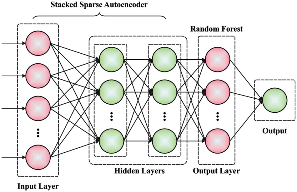
Figure 1: Framework of SSAE

Then, we and wd denotes weight matrix of encoder and decoder be and bd characterizes the bias vector. f(.)represents the activation function of AE.

The objective is to minimize the error function among the reconstructed dataset of reconstruction layer and input dataset of the visible layer. The primary term represents the average summation of square error and the next term represents weight degradation term, whereas the 3rd term represents sparse penalty term:

c(xty)=12n∑j=1n‖xj−yj‖22+λ2(‖we‖22+‖wd‖22)++β∑j=1mKL(ρ‖ρ^j)(3)

whereas:

n = the number of input dataset

λ = the weight degradation variable that controls relative momentousness of primary and 2nd second terms

β = variable control weight of sparse penalty term

m = number of neurons in hidden unit

KL(ρ||ρ^) indicates kullback-leibler divergence between mean ρ and mean ρ^jbernoulli random parameter. ρ^j represents the average activation of j hidden neuron or averaged over the trainedset and ρ indicates a sparsity variable, generally, the smallest value nearest to 0 (ρ=0.05)

KL(ρ||ρ^j) can be evaluated as follows:

KL(ρ||ρ^i)=ρ log ρρj^+(1−ρ)log (1−ρ)(1−ρ^)(4)

whereas

ρ^j=1n∑t=1nhj(x(t))(5)

The number of AE levels and hidden neurons in every level were defined using trial and error.

The higher-level feature or hidden neurons are provided to the softmax regression method, i.e., supervised learning model in DNN, and categorizes the input dataset.

Assume {(x(1),y(1)),(x(2),y(2)), (x(n),y)} tuples as input dataset, the output y could take on

f distinct classes. Then y(i)∈{1,2,3f}. The aim was to forecast the probability p(y=z|x) for =1,2,f:

hθ(x(i))=[p(y)i=1|x(i);θp(y)i=2|x(i);θ⋮p(y)i=f|x(i);θ]=1Σz=1feθZTχ(i)[eθ1Tχ(i)eθ2Tχ(i) ⋮eθfTχ(i)](6)

whereas θ1,θ2,θf are model parameter, θ=[θ1Tθ2T ⋮θfT], the term 1∑Z=1feθZTx(i) cause the distribution to sum to one and normalize it.

The cost functions of softmax regression classification mechanism are shown below:

J(θ)=−1n[∑i=1n∑z=1f1{y(i)=z}log eθZTχ(i)Σl=1feθlTχ(i)]++λ2∑i=1f∑j=0uθij2(7)

whereas 1 indicates the indicator functions, 1 {true expression} =1 and 1 {false expression} =0. The weight decayed term λ2Σi=1fΣj=0uθij2 punishes higher value of the parameter, and ιu+1 indicates dimension of feature vector χ. The cost function J(θ) is certain to have a single solution as gradient descent, L-BFGS, and so on. Because it is completely convex with the weight decay term.

3.2 Hyperparameter Tuning Using MPO Algorithm

At this stage, the MPO method is used to fine-tune the various hyperparameters of the DSSAE model. MPO, a metaheuristic influenced by nature, was created [19]. It was inspired by the vast foraging strategy adopted by ocean predators. The predator utilises both the Lévy flight and the Brownian motion techniques when hunting. Both the prey and the predator will update their location in MPO based on Lévy flight or Brownian motion. The MPO comprises four essential phases, which are outlined below.

Initialization Phase

In this section, population individual is randomly generated using the uniform distributed technique, represented X0=X min +rand(X max −X min ). X min andX max  is lower and upper limits of the parameter, correspondingly. randdenotes a random number within [0, 1]. Next, evaluate the fitness function value of each individual. At last, create Prey matrix and Elite matrix. The population individual updates its location according to the Elite and Prey matrixes [20].

MPO Optimization Scenarios

The method of optimization known as MPO can be broken down into three primary stages, each of which is determined by the distinct velocity ratios of the prey and the predator. At first, the prey is able to move more quickly than the predator. After that, both the predator and the prey move at an almost identical speed. When this occurs, the predator is able to outpace the prey. According to the rules that govern the behaviour of prey and predator movements, a particular amount of iteration time is specified and allotted to each phase.

Phase 1: In the early phase of optimization iteration, in higher velocity ratio (v≥ 10), the better strategy for predator isn’t to move at all. The mathematical modelling of this stage is given below.

Where Iter<13Max−Iter,

stepsizei=RBr⊗(Elitei−RBr⊗Preyi) i=1,…,n(8)

Preyi=Preyi+P.R⊗stepsizei

R denotes a vector of uniform random numbers within [0, 1]. Iter denotes the existing iteration number. Indicates a vector comprising random numbers according to the standard distribution demonstrating the Brownian movement. The standard Brownian movement was a random process. The step size has the features of unit variance(σ2=1) and zero mean (μ=0). The natation ⊗ illustrates the entry-wise multiplication.

Phase 2: In unit speed ratio, predators try to make transition from exploration to exploitation. Subsequently, half of the organism is earmarked for exploration and other half for exploitation.Where 13Max−Iter<Iter<23Max−Iter,

stepsizei=RBr⊗(Elitei−RBr⊗Preyi) i=1,…,n2(9)

Preyi=Elitei+P.CF⊗stepsizei

And next half of individual updates the location according to the subsequent formula:

stepsizei=RBr⊗(Elitei−RBr⊗Preyi) i=n2,…,n(10)

Preyi=Elitei+P.CF⊗stepsizei

CF=(1−IterMaxIter)(2IterMax_Iter)

RL indicates a vector of arbitrary value according to the Lévy distribution demonstrating Lévy movement. CF denotes an adaptive variable for controlling step size for predator movement. RB⊗ Elite denotes the Brownian motion of predator chasing its prey. Also, the prey upgrades its location according to the predator in Brownian movement.

Phase 3: Lower velocity ratio or if the predator moves faster than prey.

Where Iter≻23Max−Iter, individual updates its location according to the subsequent formula.

stepsizei=RLr⊗(Elitei−RLr⊗Preyi) i=1,…,n(11)

Preyi=Elitei+P.CF⊗stepsizei

RL⊗Eliteisimulated the movement of predators in the Lévy strategy.

The environmental problem could change the behavior of Marine predators, namely FADs' effect and eddy formation. Based on the study, predators often move around FAD. The FAD is regarded as local optimal and its effects as trapping at this point. Consideration of this long jumps during simulation prevents stagnation in local optimal. Consequently, FAD effects are shown in the following.

Preyi={preyi+CF[xminr+Rr⊗(x max r−xminr)]⊗Urif r≤FADsPreyi+[FADs(1−r)+r](Preyr1−Preyr2)if r≥FADs(12)

where FAD = 0.2 represents probability of FAD effects on the optimization technique. Urdenotes binary vector. rindicates a uniform random value within [0, 1]. x max randxm ln r indicates upper and lower boundaries of containing dimension. r1 and r2 subscript denotes random index of prey matrixes.

Usually, marine predators have better memories and remember places where they have been prosperous in foraging. Afterward, upgrade prey and perform FAD effects, these matrixes are estimated for fitness to upgrade the Elite. Every solution in the existing iteration is coMPOred to the preceding iteration to define its fitness. When the present solution is more fitted, it is replaced. Also, these algorithm enhances the solution quality with the lapse successful foraging. Fig. 2 displays the steps involved in MPO algorithm [21].

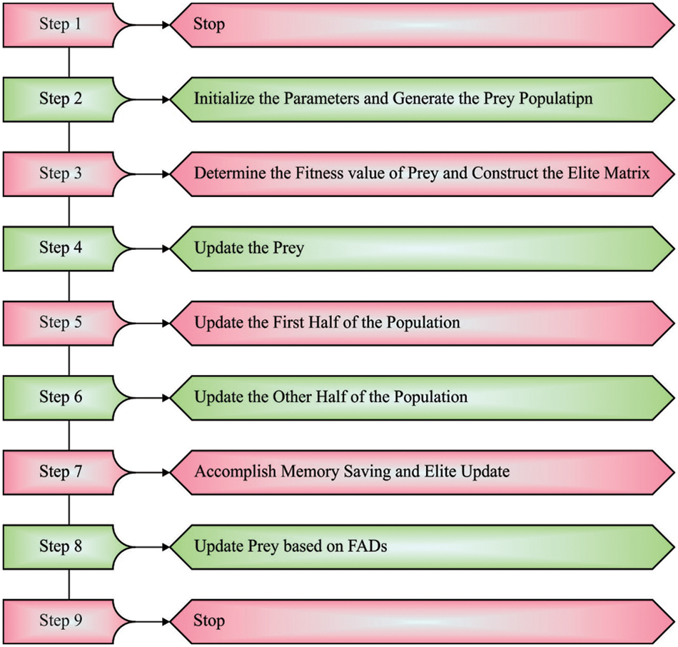
Figure 2: Steps involves in MPO algorithm

4  Performance Validation

In this section, the experimental validation of the EEHPT-DNN model is tested using eight datasets. Table 1 and Fig. 3 provides NUTE examination of the EEHPT-DNN model with recent models on eight datasets. These results inferred that the EEHPT-DNN model has offered the least values of NUTE under all normalized frequencies. At the same time, it is noticed that the EEHPT-DNN model has obtained increasing NUTE values with an increase in normalized frequencies. i.e., the value of NUTE is minimal at 1.0x normalized frequency and reaches the maximum at 4.0x normalized frequency.

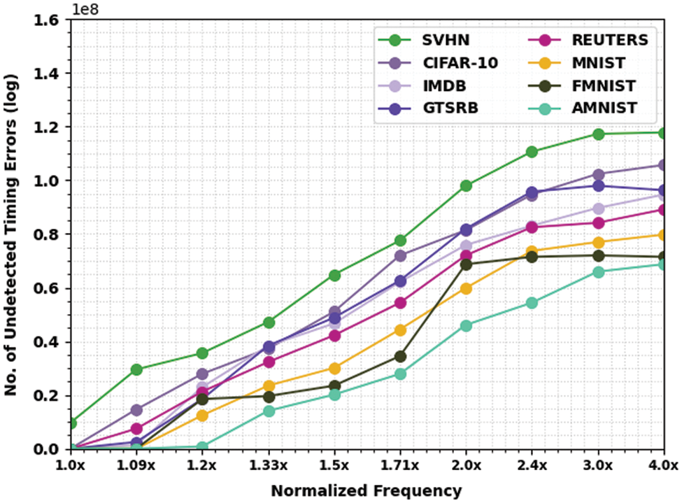
Figure 3: NUTE analysis of EEHPT-DNN approach with eight distinct datasets

Table 2 and Fig. 4 deliver NACC inspection of the EEHPT-DNN technique with recent approaches on eight datasets. These results denoted the EEHPT-DNN algorithm has the least values of NACC in all normalized frequencies. Meanwhile, it is noted that the EEHPT-DNN method has gained reduced NACC values with an increase in normalized frequencies. i.e., the value of NACC was maximum at 1.0x normalized frequency and will reach minimum at 4.0x normalized frequency.

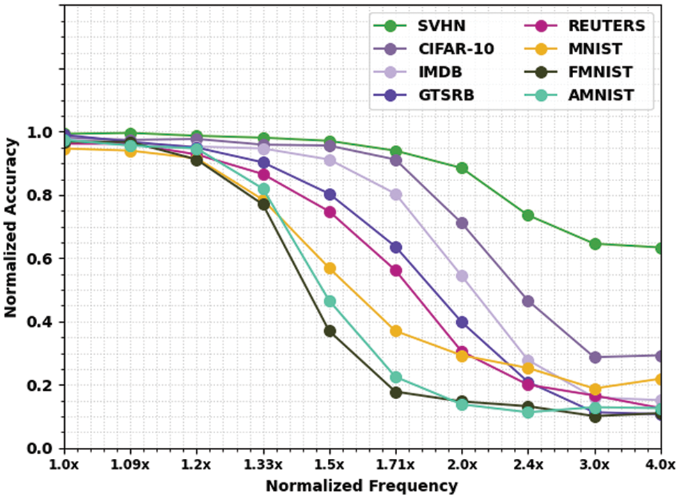
Figure 4: NACC analysis of EEHPT-DNN approach with eight distinct datasets

Table 3 provides a comparative NACC examination of the EEHPT-DNN model with existing models under SVHN dataset. The experimental outcomes implied that the EEHPT-DNN model has attained maximum NACC values on SVHN dataset at all normalized frequencies. For instance, on normalized frequency of 1.0x, the EEHPT-DNN model has offered increased NACC of 0.998 whereas the IA(PRED), IA(MRFF), BE(PRED), IA(TED), and IA(B-TPU) models have obtained reduced NACC values of 0.974, 0.973, 0, 0.979, and 0.978 respectively. Similarly, on normalized frequency of 5.0x, the EEHPT-DNN model has attained maximum NACC of 0.990 whereas the IA(PRED), IA(MRFF), BE(PRED), IA(TED), and IA(B-TPU) models have reached minimal NACC values of 0.970, 0.312, 0, 0.965, 0.965, and 0.018 respectively.

Table 4 grants a brief NACC inspection of the EEHPT-DNN approach with existing methodologies under CIFAR-10 dataset. The experimental outcomes indicate EEHPT-DNN approach has achieved maximal NACC values on SVHN dataset at all normalized frequencies. For example, on normalized frequency of 1.0x, the EEHPT-DNN technique has presented increased NACC of 0.995, whereas the IA(PRED), IA(MRFF), BE(PRED), IA(TED), and IA(B-TPU) methodologies have attained reduced NACC values of 0.959, 0.956, 0.000, 0.962, and 0.961 correspondingly. Similarly, on normalized frequency of 5.0x, the EEHPT-DNN technique has obtained maximum NACC of 0.976 whereas the IA(PRED), IA(MRFF), BE(PRED), IA(TED), and IA(B-TPU) approaches have reached minimal NACC values of 0.959, 0.292, 0.910, 0.928, and 0.004 correspondingly.

Table 5 offers a brief NACC check of the EEHPT-DNN approach with existing models under the IMDB dataset. The experimental outcomes implied that the EEHPT-DNN technique has attained maximum NACC values on SVHN dataset at all normalized frequencies. For example, on normalized frequency of 1.0x, the EEHPT-DNN approach has rendered increased NACC of 0.981 whereas the IA (PRED), IA (MRFF), BE (PRED), IA (TED), and IA (B-TPU) methodologies have acquired reduced NACC values of 0.975, 0.965, 0.000, 0.977, and 0.959 correspondingly. Also, on normalized frequency of 5.0x, the EEHPT-DNN technique has reached maximum NACC of 0.977 whereas the IA (PRED), IA (MRFF), BE (PRED), IA (TED), and IA (B-TPU) approaches have reached minimal NACC values of 0.968, 0.309, 0.905, 0.857, and 0.002 correspondingly.

Table 6 offers the detailed NACC analysis of the EEHPT-DNN approach with existing techniques under GTSRB dataset. The experimental outcomes implied that the EEHPT-DNN approach has reached maximum NACC values on SVHN dataset at all normalized frequencies. For example, on normalized frequency of 1.0x, the EEHPT-DNN model has offered increased NACC of 0.978 whereas the IA (PRED), IA (MRFF), BE (PRED), IA (TED), and IA (B-TPU) methodologies have acquired reduced NACC values of 0.971, 0.980, 0.000, 0.973, and 0.955 correspondingly. Similarly, on normalized frequency of 5.0x, the EEHPT-DNN technique has attained maximum NACC of 0.976 whereas the IA (PRED), IA (MRFF), BE (PRED), IA (TED), and IA (B-TPU) approaches have reached minimal NACC values of 0.956, 0.287, 0.846, 0.890, and 0.008 correspondingly.

Table 7 offers a comprehensive NACC analysis of the EEHPT-DNN technique with existing methodologies under REUTERS dataset. The experimental outcomes denoted the EEHPT-DNN algorithm has achieved maximum NACC values on SVHN dataset at all normalized frequencies. For example, on normalized frequency of 1.0x, the EEHPT-DNN approach has rendered increased NACC of 0.978 whereas the IA (PRED), IA (MRFF), BE (PRED), IA (TED), and IA (B-TPU) algorithms have reached reduced NACC values of 0.972, 0.975, 0.000, 0.962, and 0.967 correspondingly. Also, on normalized frequency of 5.0x, the EEHPT-DNN method has obtained maximum NACC of 0.994 whereas the IA (PRED), IA (MRFF), BE (PRED), IA (TED), and IA (B-TPU) approaches have reached minimal NACC values of 0.945, 0.298, 0.945, 0.944, and 0.179 correspondingly.

Table 8 presents a comparative NACC examination of the EEHPT-DNN method with existing approaches under MINIST dataset. The experimental outcomes implied that the EEHPT-DNN approaches have reached maximum NACC values on SVHN dataset at all normalized frequencies. For example, on normalized frequency of 1.0x, the EEHPT-DNN method has rendered increased NACC of 0.999, whereas the IA (PRED), IA (MRFF), BE (PRED), IA (TED), and IA (B-TPU) approaches have achieved reduced NACC values of 0.962, 0.969, 0.000, 0.960, and 0.952 correspondingly. Similarly, on normalized frequency of 5.0x, the EEHPT-DNN method has obtained maximum NACC of 0.979 whereas the IA (PRED), IA (MRFF), BE (PRED), IA (TED), and IA (B-TPU) methods have reached minimal NACC values of 0.953, 0.294, 0.942, 0.968, and 0.216 correspondingly.

Table 9 portrays a comparative NACC analysis of the EEHPT-DNN approach with existing approaches under FMINIST dataset. The experimental outcomes denote the EEHPT-DNN approach has obtained maximum NACC values on SVHN dataset at all normalized frequencies. For example, on normalized frequency of 1.0x, the EEHPT-DNN algorithm has presented increased NACC of 0.997 whereas the IA (PRED), IA (MRFF), BE (PRED), IA (TED), and IA (B-TPU) approaches have obtained reduced NACC values of 0.972, 0.976, 0, 0.969, and 0.973 correspondingly. Also, on normalized frequency of 5.0x, the EEHPT-DNN approach has attained maximum NACC of 0.992 whereas the IA (PRED), IA (MRFF), BE (PRED), IA (TED), and IA (B-TPU) algorithms have reached minimal NACC values of 0.953, 0.292, 0.952, 0.949, and 0.007 correspondingly.

Table 10 demonstrates a complete NACC analysis of the EEHPT-DNN algorithm with existing approaches under AMINIST dataset. The experimental outcomes indicated the EEHPT-DNN approach has acquired maximum NACC values on SVHN dataset at all normalized frequencies. For example, on normalized frequency of 1.0x, the EEHPT-DNN method has presented increased NACC of 0.981, whereas the IA (PRED), IA (MRFF), BE (PRED), IA (TED), and IA (B-TPU) algorithms have attained reduced NACC values of 0.961, 0.951, 0.000, 0.952, and 0.971 correspondingly. Likewise, on normalized frequency of 5.0x, the EEHPT-DNN technique has obtained maximum NACC of 0.991 whereas the IA (PRED), IA (MRFF), BE (PRED), IA (TED), and IA (B-TPU) approaches have reached minimal NACC values of 0.960, 0.284, 0.940, 0.944, and 0.118 correspondingly.

An overall comparison study of the EEHPT-DNN model with recent models under eight datasets is given in Fig. 5. The figure implied that the EEHPT-DNN model has shown outperforming performance over other models on all the test datasets.

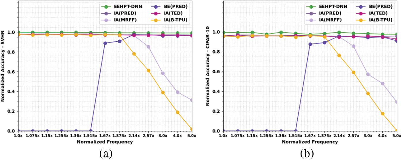
Figure 5: Comparative analysis of EEHPT-DNN approach (a) SVHN, (b) CIFAR-10, (c) IMDB, (d) GTSRB, (e) REUTERS, (f) MNIST, (g) FMNIST, (h) AMNIST

5  Conclusion

This paper proposes a novel developed EEHPT-DNN technique for Variation-Tolerant Near-Threshold Processor. The presented EEHPT-DNN model employs AI techniques to improve the energy efficiency of AI. The model emphasises the effects of embedded systems near the network’s edge. For the development of a variation-tolerant NT processor, the suggested model utilised the DSSAE paradigm. Due to the time-consuming and arduous nature of tuning hyperparameters through trial and error, the MPO approach is used to alter the hyperparameters associated with the DSSAE model. In order to demonstrate that the presented EEHPT-DNN model has a higher degree of functionality, a thorough simulation assessment has been conducted, and the results of this evaluation have been analysed with respect to a number of criteria. Compared to other DL models, the EEHPT-DNN model delivered superior outcomes, according to the findings of the comparison study.

Funding Statement: The authors received no specific funding for this study.

Conflicts of Interest: The authors declare that they have no conflicts of interest to report regarding the present study.

References

1. W. Shan, X. Shang, X. Wan, H. Cai, C. Zhang et al., “A wide-voltage-range half-path timing error-detection system with a 9-transistor transition-detector in 40-nm CMOS,” IEEE Transactions on Circuits and Systems I: Regular Papers, vol. 66, no. 6, pp. 2288–2297, 2019. [Google Scholar]

2. P. Pandey, P. Basu, K. Chakraborty and S. Roy, “GreenTPU: Improving timing error resilience of a near-threshold tensor processing unit,”in Proc. of the 56th ACM/IEEE Design Automation Conf. (DAC), IEEE, Las Vegas, NV, USA, pp. 1–6, 2019. [Google Scholar]

3. S. Wang, C. Chen, X. Y. Xiang and J. Y. Meng, “A Variation-tolerant near-threshold processor with instruction-level error correction,” IEEE Transactions on Very Large Scale Integration (VLSI) Systems, vol. 25, no. 7, pp. 1993–2006. 2017. [Google Scholar]

4. P. Pandey, P. Basu, K. Chakraborty and S. Roy, “GreenTPU: Predictive design paradigm for improving timing error resilience of a near-threshold tensor processing unit,” IEEE Transactions on Very Large Scale Integration (VLSI) Systems, vol. 28, no. 7, pp. 1557–1566, 2019. [Google Scholar]

5. J. Koo, E. Park, D. Kim, J. Park, S. Ryu et al., “Low-overhead, one-cycle timing-error detection and correction technique for flip-flop based pipelines,” IEICE Electronics Express, vol. 2019, pp. 16-20190180–1620190196, 2019. [Google Scholar]

6. R. G. Rizzo, V. Peluso, A. Calimera, J. Zhou and X. Liu, “Early bird sampling: A short-paths free error detection-correction strategy for data-driven VOS, “in Proc. of the IFIP/IEEE Int. Conf. on Very Large Scale Integration (VLSI-SoC), IEEE, Abu Dhabi, United Arab Emirates, pp. 1–6, 2017. [Google Scholar]

7. V. Bhatnagar, M. K. Pandey and S. Pandey, “A variation tolerant nanoscale sram for low power wireless sensor nodes,” Wireless Personal Communications, vol. 124, pp. 3235–3251, 2022. [Google Scholar]

8. E. Mani, E. Abbasian, M. Gunasegeran and S. Sofimowloodi, “Design of high stability, low power and high speed 12 T SRAM cell in 32-nm CNTFET technology,” AEU-International Journal of Electronics and Communications, vol. 154, pp. 154308, 2022. [Google Scholar]

9. S. Wang, C. Chen, X. Xiang and J. Meng, “A Metastability-immune error-resilient flip-flop for near-threshold variation-tolerant designs,” IEICE Electronics Express, vol. 14, no. 11, pp. 20170353–20170353, 2017. [Google Scholar]

10. P. Sharma and B. P. Das, “Design and analysis of leakage-induced false error tolerant error detecting latch for sub/near-threshold applications,” IEEE Transactions on Device and Materials Reliability, vol. 20, no. 2, pp. 366–375, 2020. [Google Scholar]

11. Y. Lin, S. Zhang. and N. R. Shanbhag, “A rank decomposed statistical error compensation technique for robust convolutional neural networks in the near threshold voltage regime,” Journal of Signal Processing Systems, vol. 90, no. 10, pp. 1439–1451, 2018. [Google Scholar]

12. N. D. Gundi, P. Pandey, S. Roy and K. Chakraborty, “Implementing a timing error-resilient and energy-efficient near-threshold hardware accelerator for deep neural network inference,” Journal of Low Power Electronics and Applications, vol. 12, no. 2, pp. 1–32, 2022. [Google Scholar]

13. Y. Lin and J. R. Cavallaro, “Energy-efficient convolutional neural networks via statistical error compensated near threshold computing,” in Proc. IEEE Int. Symp. on Circuits and Systems (ISCAS), Florence, Italy, pp. 1–5, 2018. [Google Scholar]

14. J. Wang, W. W. Liang, Y. H. Niu, L. Gao and W. G. Zhang, “Multi-dimensional optimization for approximate near-threshold computing,” Frontiers of Information Technology & Electronic Engineering, vol. 21, no. 10, pp. 1426–1441, 2020. [Google Scholar]

15. I. Tsiokanos, L. Mukhanov, D. S. Nikolopoulos and G. Karakonstantis, “Significance-driven data truncation for preventing timing failures,” IEEE Transactions on Device and Materials Reliability, vol. 19, no. 1, pp. 25–36, 2019. [Google Scholar]

16. T. T. Zhu, J. Y. Meng, X. Y. Xiang and X. L. Yan, “Error-resilient integrated clock gate for clock-tree power optimization on a wide voltage IoT processor,” IEEE Transactions on Very Large Scale Integration (VLSI) Systems, vol. 25, no. 5, pp. 1681–1693, 2019. [Google Scholar]

17. T. Zhu, X. Xiang, C. Chen and J. Meng, “SGERC: A self-gated timing error resilient cluster of sequential cells for wide-voltage processor,” IEICE Electronics Express, pp. 20170214–20170218, 2017. [Google Scholar]

18. S. Akhila, S. Zubeda and R. Shashidhara, “DS2AN: Deep stacked sparse autoencoder for secure and fast authentication in HetNets,” Security and Privacy, vol. 5, no. 3, pp. e208, 2022. [Google Scholar]

19. M. A. Soliman, H. M. Hasanien and A. Alkuhayli, “Marine predators algorithm for parameters identification of triple-diode photovoltaic models,” IEEE Access, vol. 8, pp. 155832–155842, 2020. [Google Scholar]

20. M. Mustaqeem and S. Kwon, “A CNN assisted enhanced audio signal processing for speech emotion recognition,” Sensors, vol. 20, no. 1, pp. 1–15, 2020. [Google Scholar]

21. Z. Tarek, M. Y. Shams, A. M. Elshewey, E. M. El-kenawy, A. Ibrahim et al., “Wind power prediction based on machine learning and deep learning models,” Computers, Materials & Continua, vol. 74, no. 1, pp. 715–732, 2023. [Google Scholar]