Lightweight Method for Plant Disease Identification Using Deep Learning

1  Introduction

In agricultural production, plant diseases are a leading cause of crop yield reduction. In actual production, the identification of plant diseases mainly depends on the farmers’ long-term experience. For large agricultural lands with a variety of crops, the identification of plant diseases is time consuming and laborious. Moreover, the identification of plant diseases is time sensitive, has a small detection range, and is not reliable. The use of computer vision to analyze images of crop leaves to identify plant diseases has good application prospects in the agricultural production field. Numerous scholars have attempted to use deep learning methods to identify crop pests and diseases, assist in the prevention and diagnosis of plant diseases, and promote the rapid development of agriculture [1–3].

Krishnamoorthy et al. [4] used the InceptionResNetV2 model along with a migration learning approach to identify diseases in rice leaf images and obtained a remarkable accuracy of 95.67%. Tiwari et al. [5] performed migration learning using a pre-trained model (e.g., VGG19) for the early and late blight of potato to extract relevant features from the datasets. Their perceptual logistic regression, with the help of multiple classifiers, performed exceptionally well in terms of classification accuracy, significantly outperforming other classifiers and yielding 97.8% accuracy. Wen et al. [6] proposed a large-scale multi-class pest recognition network model. They introduced a convolutional block attention model in the baseline network model and mixed the cross-feature channel domain with the feature space domain to realize model extraction and represent key features in both channel and space dimensions; the key features are used to enhance the extraction and representation of differentiated features in the network. Additionally, they introduced the cross-layer non-local module among the multiple feature extraction layers to improve the model’s fusion of multi-scale features. The Top1 recognition accuracy was 88.62% and 74.67% on 61 types of disease datasets and 102 types of pest datasets, respectively.

The above studies employed classical convolutional neural networks (CNNs) to improve the crop pest and disease identification accuracy. The accuracy of classical CNN models, such as AlexNet [7], VGG [8], ResNet [9], and GoogleNet [10], is being constantly improved, and their network depth is increasing and becoming more profound [11]. Moreover, the number of parameters is increasing, which is consequently increasing the computation. Bao et al. [12] designed a lightweight CNN model called SimpleNet to identify wheat diseases, such as erysipelas, and achieved 94.1% recognition accuracy. Hong et al. [13] improved the lightweight CNN ShuffleNetV2 0.5x, which can effectively identify the disease types of many crop leaves. However, the recognition accuracy of lightweight CNNs is generally lower than that of large network models [14]. Consequently, improving the model’s recognition accuracy while keeping it lightweight is a pressing issue during the design of a lightweight CNN.

Based on the above problems, this study improves on ShuffleNetV2, aiming to improve the recognition accuracy of the model while keeping it lightweight. The key contributions of this study are as follows:

▪   The depthwise convolution in the basic module of ShuffleNetV2 is replaced with mixed depthwise convolution (MixDWConv) to capture crop pest images at different resolutions.

▪   The efficient channel attention (ECA) module is added to the ShuffleNetV2 model network structure to enhance the channel features.

▪   The ReLU6 activation function is introduced to prevent the generation of large gradients.

The proposed lightweight CNN is highly suitable for deploying the model on embedded resource-constrained devices, such as mobile terminals, which assists in realizing the accurate identification of plant diseases in real time. Additionally, it has robust engineering utility and high research value.

The remainder of this paper is structured as follows. Section 2 presents the literature review and the baseline model. Section 3 describes the proposed model. Section 4 discusses the experimental results and ablation study. Finally, Section 5 presents the conclusions.

2  Related Work

Mohanty et al. [15] were the first to use deep learning methods for crop disease recognition, based on two classical CNN models, AlexNet and GoogleNet, for migration learning. They demonstrated that deep learning methods exhibit high performance and usability in crop disease recognition, providing a direction for subsequent research. Too et al. [16] performed migration learning using various classical CNN models. However, the network models in the above studies are deep and complex and cannot be effectively employed for agricultural production practices on low-performing edge mobile terminal devices with limited computational resources.

Sun et al. [17] proposed various improved AlexNet models using batch normalization, null convolution, and global pooling, which reduced the model parameters and improved the recognition accuracy. Su et al. [18] proposed a model for grapevine leaf disease recognition based on a migration learning model training approach; the accuracy of their model is 10 percentage points higher than that of models based on ordinary training, and their model can be deployed to mobile terminals. Xu et al. [19] proposed a ResNet50 CNN image recognition method based on an improved Adam optimizer and achieved a classification accuracy of 97.33% for real scenes. Liu et al. [20] proposed an improvement to the classical lightweight CNN SqueezeNet and significantly reduced the memory requirements of the model parameters and the model computation, and their proposed model rapidly converged. Jia et al. [21] proposed a method for plant leaf disease identification based on lightweight CNNs. Their improved network exhibited high disease identification accuracy (99.427%) while occupying a small memory space. Li et al. [22] proposed a lightweight crop disease recognition method based on ShuffleNet V2. For their method, the number of model parameters was about 2.95 × 105 and the average disease recognition accuracy was 99.24%. Guo et al. [23] proposed a multi-sensory field recognition model based on AlexNet for mobile platforms, setting convolution kernels of different sizes for the first layer of AlexNet models and extracting multiple features to characterize the dynamic changes of diseases in a comprehensive manner. Liu et al. [24] proposed two lightweight crop disease recognition methods based on MobileNet and Inception V3, which were selected based on the recognition accuracy, computational speed, and model size, and they were implemented for leaf detection on mobile phones.

2.1 ShuffleNetV2 Model Structure

The ShuffleNetV1 network is a high-performance lightweight CNN that was proposed by the Megvii Technology team in 2017. The essential metrics for the neural network architecture design have not only computational complexity [25] but also factors such as memory access and platform characteristics. The number of parameters in ShuffleNetV1 can be reduced using grouped convolution, but the number of groups is too large to increase the memory access. Based on the ShuffleNetV1 model, Ma et al. [26] proposed four lightweight guidelines: (1) the memory access is minimized when the input and output channels of the convolutional layers are the same; (2) grouped convolution with abundant groups increases the memory access; (3) fragmentation operations are not friendly to parallel acceleration; and (4) the memory and time consumption stemming from the element-by-element operations cannot be ignored. Based on the guidelines, the basic module of ShuffleNetV1 was improved and the ShuffleNetV2 network was constructed, as shown in Table 1.

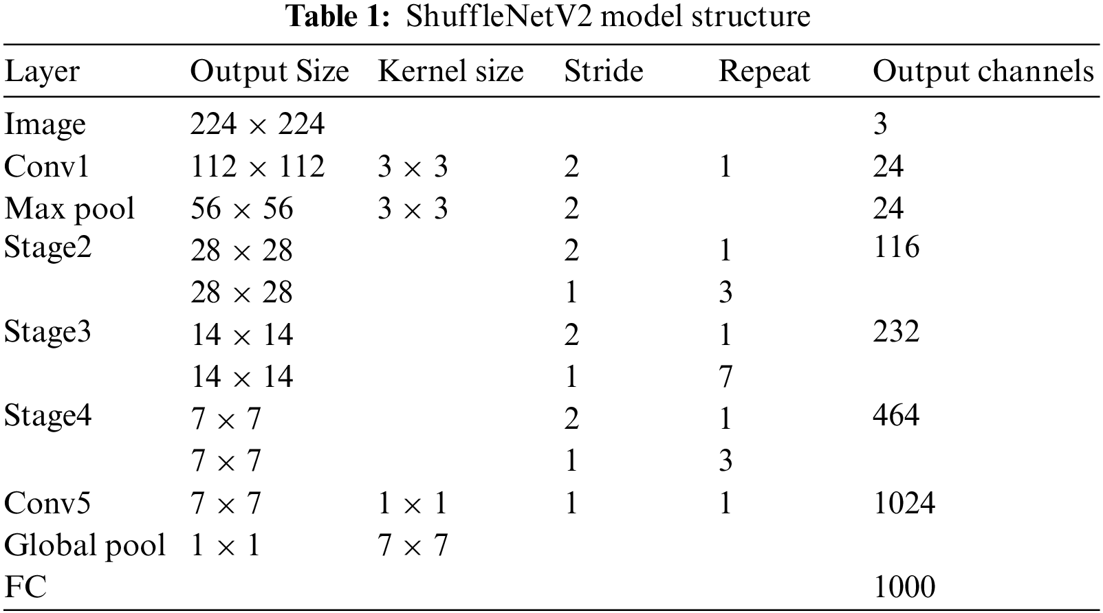
The ShuffleNetV2 network includes the Conv1 layer, Max Pool layer, Stage2 layer, Stage3 layer, Stage4 layer, Conv5 layer, Global Pool layer, and FC layer. The Stage2, Stage3, and Stage4 layers comprise stacked basic modules. The Stage2 and Stage4 layers are stacked with four basic modules, and the Stage3 layer is stacked with eight basic modules. The first basic module in each stage has a stride size of 2, which is mainly used for downsampling, and the other basic modules have a stride size of 1.

2.2 ShuffleNetV2 Basic Module

Fig. 1a displays the basic module of ShuffleNetV2, where the input features are equally divided into two branches after the channel split operation. The left branch does not perform any constant operation mapping. The right branch undergoes 1 × 1 ordinary convolution, 3 × 3 depthwise separable convolution (DWConv), and 1 × 1 ordinary convolution to yield the right branch output. The left and right branches have equal number of input and output channels. They are merged by the Concat operation, and then, the channel shuffle operation is performed to ensure that the feature information of the left and right branches is fully fused. Fig. 1b shows the downsampling module of ShuffleNetV2. The feature maps are input into the two branches. The left branch undergoes 3 × 3 depthwise separable convolution with stride size two and 1 × 1 standard convolution. The right branch undergoes the same operations as those in (a) but the stride size of the depthwise separable convolution is 2. The left and right branches are merged using the Concat operation, and then, the channel shuffle operation is performed to fuse the information of the different channels.

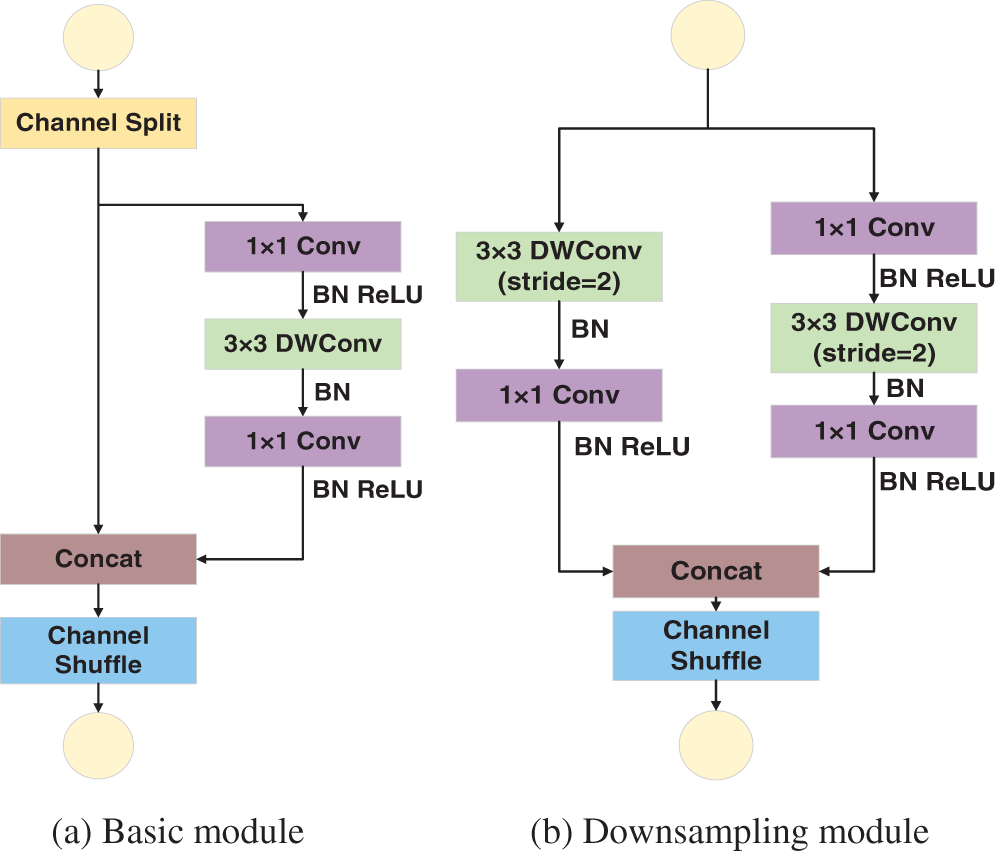
Figure 1: ShuffleNetV2 basic module

2.2.1 Depthwise Separable Convolution (DWConv)

Depthwise separable convolution [27] is performed once for the depthwise and pointwise convolutions. The structure and process are shown in Fig. 2. The depthwise convolution processes each layer of the input information with the same number of convolution kernels. Additionally, it processes the spatial information for the aspect direction without considering the cross-channel information. The pointwise convolution performs 1 × 1 convolution on the depthwise convolution output and is only concerned with the cross-channel information.

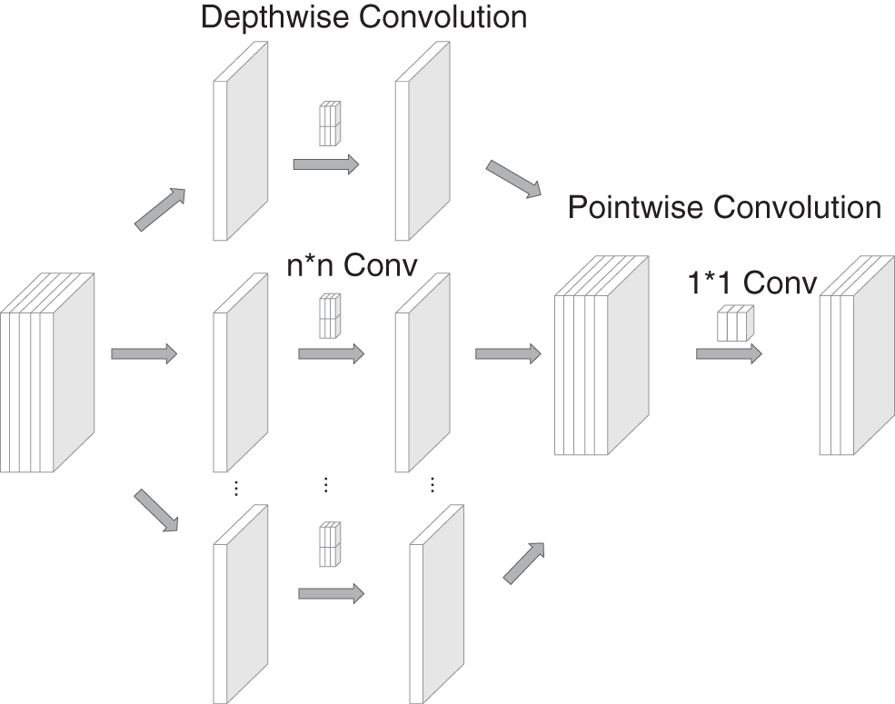
Figure 2: Depthwise separable convolution

The multiplication of the standard convolution is computed as

(Dk⋅Dk⋅M)⋅(N⋅DF⋅DF)(1)

where Dk is the size of the convolution kernel, M is the number of input feature channels, N is the number of output feature channels, and DF is the size of the output feature map.

The number of parameters for the standard convolution is

Dk⋅Dk⋅M⋅N(2)

The multiplication of the depthwise separable convolution is computed as

(Dk⋅Dk)⋅(M⋅DF⋅DF)+M⋅(N⋅DF⋅DF)(3)

The number of parameters for the depthwise separable convolution is

Dk⋅Dk⋅M+1⋅1⋅M⋅N(4)

The ratio of the multiplication of the depthwise separable convolution to the standard convolution is

(Dk⋅Dk)⋅(M⋅DF⋅DF)+M⋅(N⋅DF⋅DF)(Dk⋅Dk⋅M)⋅(N⋅DF⋅DF)=1N+1Dk2(5)

The ratio of the number of parameters of the depthwise separable convolution to the standard convolution is

Dk⋅Dk⋅M+M⋅NDk⋅Dk⋅M⋅N=1N+1Dk2(6)

N is the number of channels in the output; thus, it is negligible. Dk is the size of the convolution kernel, which is typically set as 3. The depthwise separable convolution is 1/9 times larger than the standard convolution in terms of both computation and number of parameters. Compared to the traditional convolution operation, the depthwise separable convolution reduces the number of parameters and improves the model training speed.

2.2.2 Channel Shuffle

The channel shuffle operation not only facilitates the information exchange among different channels but also reduces the computational effort of the model [28]. As shown in Fig. 3, group convolution restricts the information exchange across groups, which could lead to the group information closure phenomenon. The channel shuffle operation divides the input feature map into several groups according to the channels, divides each group into subgroups, and randomly selects subgroups from each group to form a new feature map so that information can be exchanged across groups. The information flow between the channel groups is improved, thus ensuring correlation between the input and output channels.

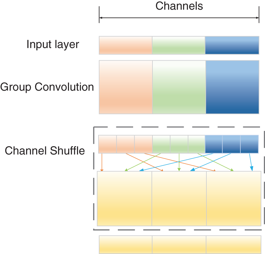
Figure 3: Channel shuffle

3  Method

Based on the characteristics of plant diseases, ShuffleNetV2 is selected as the backbone network in this study. Depthwise convolution only uses a single convolution kernel to extract image features, which is not suitable for image recognition in different resolutions, and thus, MixDWConv is used instead of depthwise convolution in the ShuffleNetV2 basic module. To strengthen the channel features, the ECA module is introduced in the ShuffleNetV2 network structure. The ReLU activation function easily yields large gradients in the network training process. Therefore, the ReLU activation function is replaced by the ReLU6 activation function.

The lightweight model ShuffleNetV2 is improved to overcome the problems of the large number of parameters and the high model complexity of the classical CNN. As shown in Fig. 4, the input is a 3 × 224 × 224 image. The image first undergoes an ordinary convolution with a convolutional kernel size of 3 and stride size of 2 for feature extraction of the detail part of the image. Max Pool represents a convolutional kernel size of 3 and a stride size of 2 for the output of the upper layer to perform the maximum pooling operation for realizing the feature dimensionality reduction. ShuffleNetV2 unit1 indicates that the output of the upper layer is repeated once with the downsampling module and three times with the basic module. ECA block denotes that the output of the upper layer is processed by the ECA module to strengthen the channel features. ShuffleNetV2 unit2 indicates that the output of the upper layer is repeated once with the downsampling module and seven times with the basic module. Then, the output of ShuffleNetV2 unit2 is processed by the ECA module. ShuffleNetV2 unit3 performs the same operation as ShuffleNetV2 unit1. The output of ShuffleNetV2 unit3 is processed by the ECA module. The output of the ECA module is subjected to one convolutional kernel size for ordinary convolutional up-dimensioning. The final output is obtained after passing through global average pooling (GAP) and fully connected layers.

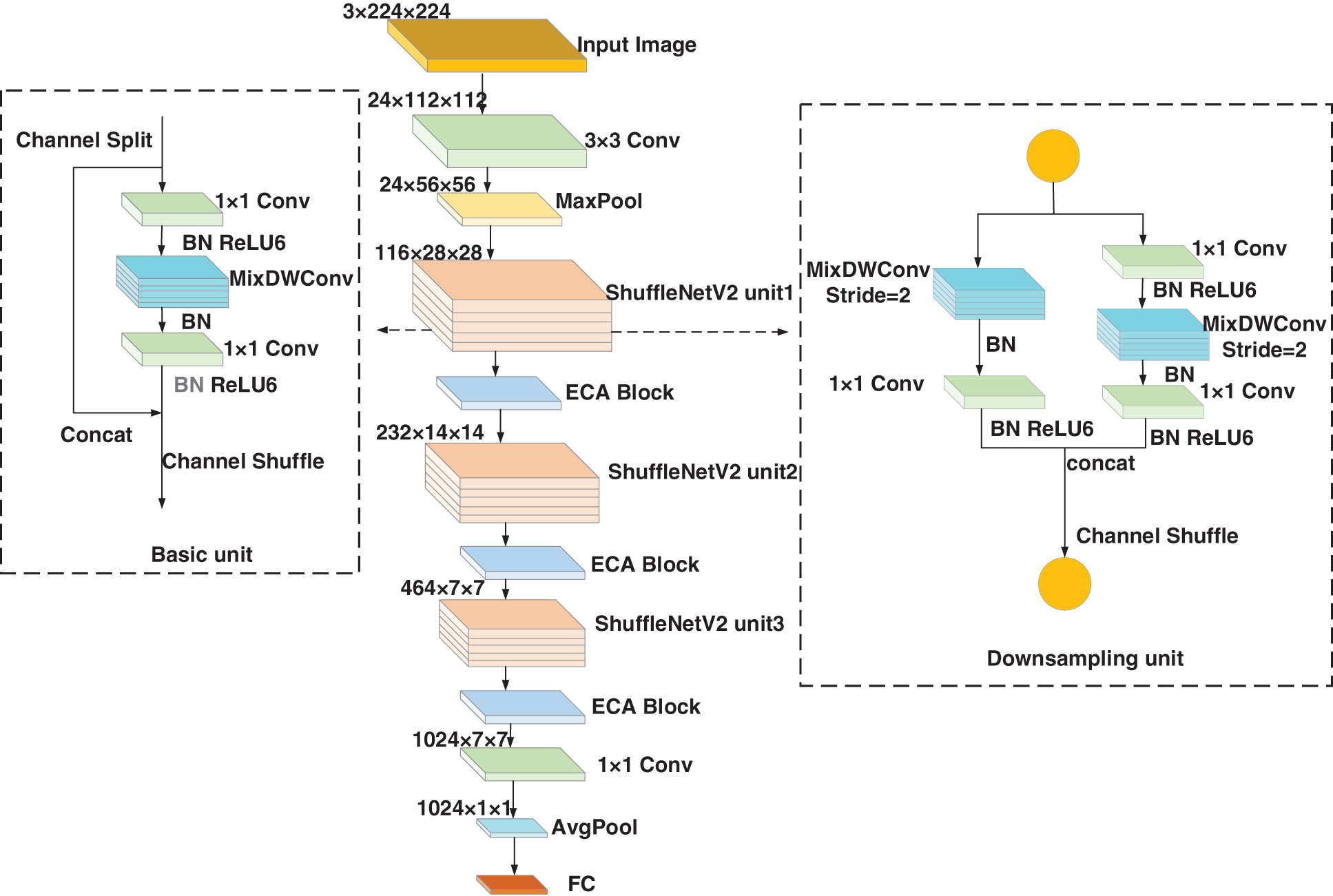
Figure 4: Structure of the improved ShuffleNetV2 network

In the basic and downsampling modules, the proposed model uses MixDWConv instead of the depthwise convolution of the ShuffleNetV2 model. Furthermore, the ReLU6 activation function is used instead of the ReLU activation function. The MixDWConv, ECA module, and ReLU6 activation function are further elaborated below.

3.1 Mixed Depthwise Convolution

When designing CNNs, one of the most critical and easily overlooked points regarding depthwise convolution is the size of the convolutional kernel. Although traditional depthwise convolution generally employs a convolutional kernel size of 3, recent studies [29,30] have suggested that the model’s accuracy could be improved by employing larger convolutional kernels, such as 5 × 5 and 7 × 7.

Based on MobileNets, Tan et al. [31] systematically investigated the effect of the convolutional kernel size. In Fig. 5, the convolution kernel sizes represented by the dots, from left to right, are 3 × 3, 5 × 5, 7 × 7, 9 × 9, 11 × 11, and 13 × 13, and the size of the dots represents the model size. As shown in Fig. 5, the larger the convolution kernel, the greater the number of parameters, which increases the model size. The accuracy of the convolution kernel size substantially improves from the 3 × 3 to 7 × 7 models, and the accuracy significantly decreases when the convolution kernel is 9 × 9, which indicates that the accuracy is low for large convolution kernel sizes, exhibiting the limitation of a single convolution kernel. For a model to achieve high accuracy and efficiency, large convolutional kernels are required to capture high-resolution patterns and small convolutional kernels are required to capture low-resolution patterns. Therefore, Tan et al. [31] proposed MixDWConv that is a mixture of convolution kernels of different sizes in one convolution operation, which enables the capture of different images at different resolutions.

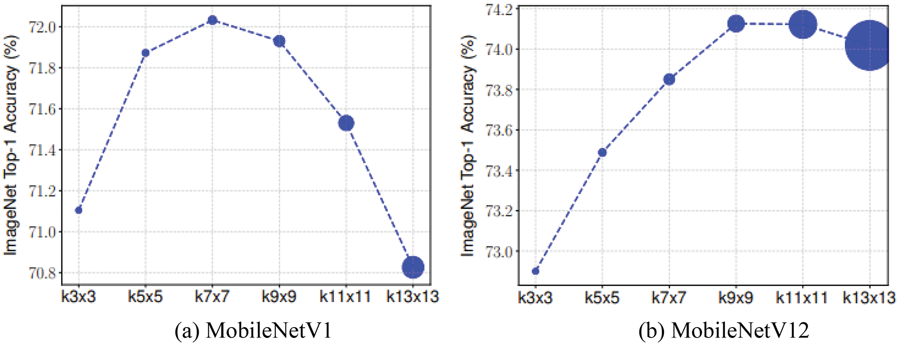
Figure 5: Relationship between accuracy and convolution kernel size

As stated in Section 2.3, while the 3 × 3 depthwise convolution is used in the ShuffleNetV2 basic module, the proposed model employs MixDWConv. As shown in Fig. 4, MixDWConv is considered as a simple implantation instead of the ordinary depthwise convolution. Fig. 6 displays the structure of MixDWConv. The ordinary depthwise convolution uses convolution kernels of the same size for all the channels. In contrast, MixDWConv divides all channels into groups and applies convolution kernels of different sizes to different groups. MixDWConv can easily obtain different patterns from the input image, allowing the model to achieve high accuracy.

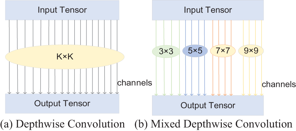
Figure 6: Structure of MixDWConv

The MixDWConv operation involves several variables.

▪   Number of groups g: The number of groups determines how many convolutional kernels of different sizes need to be used for the input tensor. In literature [29], the best results have been achieved with g = 4. Similarly, in our experiments, ShuffleNetV2 affords the best results when g = 4. Subsequent selection of the number of groups in MixDWConv is verified in Section 4.5.

▪   Size of convolutional kernels in each group: The size of the convolutional kernels can be arbitrary in theory, but without restriction, the size of convolutional kernels in two groups may be the same, which is equivalent to merging into one group. Therefore, different convolution kernel sizes need to be set for each group. The restricted convolution kernel size is set as 3 × 3 and is monotonically increased by 2 for each group, i.e., the size of the convolution kernel for the ith group is 2i + 1. For example, in this experiment, g = 4 and the convolution kernel size is {3 × 3, 5 × 5, 7 × 7, 9 × 9}. For an arbitrary number of groupings, the convolution kernel size is already determined, which simplifies the design process.

▪   Number of channels in each group: The equal division method is used, i.e., the number of channels is divided into four equal groups, and the number of channels in each group is the same.

3.2 ECA Block

The channel attention mechanism can effectively improve the performance of CNNs. Most attention mechanisms can improve the network accuracy, but they increase the computational burden. Wang et al. [32] proposed the ECA module, which is a channel attention module. In contrast to other channel attention mechanisms, the ECA module can improve the performance of CNNs without increasing the computational burden. Fig. 7 shows the structure of the ECA module. First, the input dimension is a feature map with dimension of H × W × C. The input feature map is compressed with spatial features, and the feature map of 1 × 1 × C is obtained using GAP. The compressed feature map is learned with channel features, and the importance between different channels is learned using 1 × 1 convolution. The output dimension is 1 × 1 × C. Finally, the feature map of channel attention 1 × 1 × C and the original input feature map H×W×C are multiplied channel-by-channel to yield the feature map with channel attention. The ECA module is introduced in the proposed model to enhance the channel features and improve the network’s performance without increasing the number of model parameters.

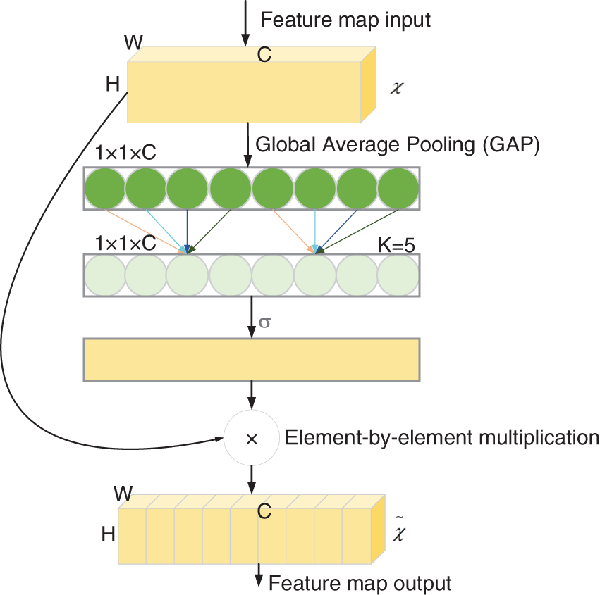
Figure 7: ECA module structure

3.3 Activation Function ReLU6

The primary role of the activation function is to provide the network with the ability of nonlinear modeling to address the deficiency of the model representation capability, which has a crucial role in neural networks [33]. The ReLU activation function is simple to compute and allows the sparse representation of the network, but it is fragile in the network training process. As shown in Eq. (8), the ReLU activation function sets all the negative values to 0 and leaves the other values unchanged, which causes the network to considerably vary in the range of weights during the training process and be prone to the phenomenon of “neural necrosis” [34], which consequently decreases the quantization accuracy. Compared to the ReLU activation function, ReLU6 can prevent the generation of large gradients. Therefore, the ReLU6 activation function is used in the improved ShuffleNetV2 basic module proposed herein. The chain rule formula is as follows.

∂loss∂w=∂loss∂y∗∂y∂B∗∂B∂w=∂loss∂y∗∂y∂B∗A(7)

Here,∂y∂B denotes the gradient of ReLU or ReLU6, and the relationship between A and B is linear. When using ReLU as the activation function, as shown in Fig. 8a, B is too large and A is likely to be too large, which results in an extremely large gradient ∂loss∂w and leads to a large difference in the weights. In ReLU6, as shown in Fig. 8b, the positive interval is partitioned; when B > 6, ∂y∂B will be 0, i.e., when A is too large, B will be greater than 6, thus making ∂loss∂w=∂y∂B=0, which prevents the generation of large gradients.

ReLU={x,(x≥0)0,(x<0)(8)

ReLU6={0,(x≤0)x,(0<x<6)6,(x≥6)(9)

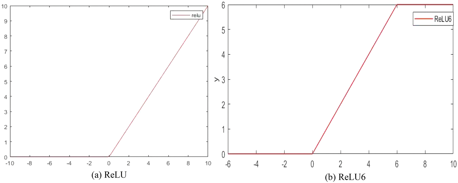
Figure 8: Comparison of ReLU and ReLU6 activation functions

4  Experiments

4.1 Experimental Environment

The experiment was performed using an Intel (R) Core (TM) i7-8700 CPU processor with the Windows 10 operating system, Pytorch 1.7.1 deep learning framework, and PyCharm development platform. During the training process, to ensure scientific and reliable results, in all experiments, the stochastic gradient descent optimizer is used for parameter updation, the loss function is the cross-entropy function, the number of iterations is 30, and the batch size is 64.

4.2 Datasets and Pre-processing

The experiments are performed on the publicly available dataset PlantVillage [35] to identify 25 types of plant diseases in five crops. Some of the images are shown in Fig. 9.

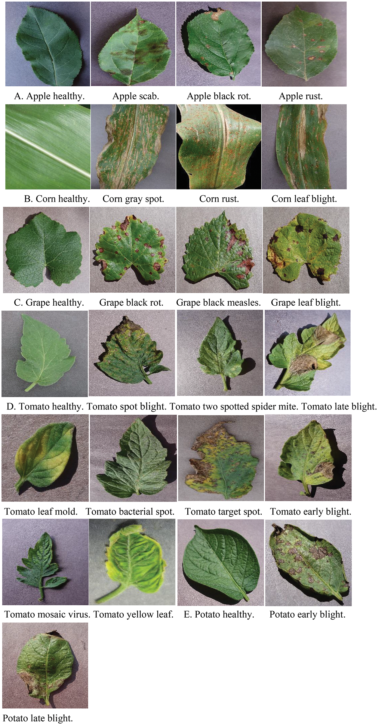
Figure 9: Diseased leaves of apple, corn, grape, tomato, and potato

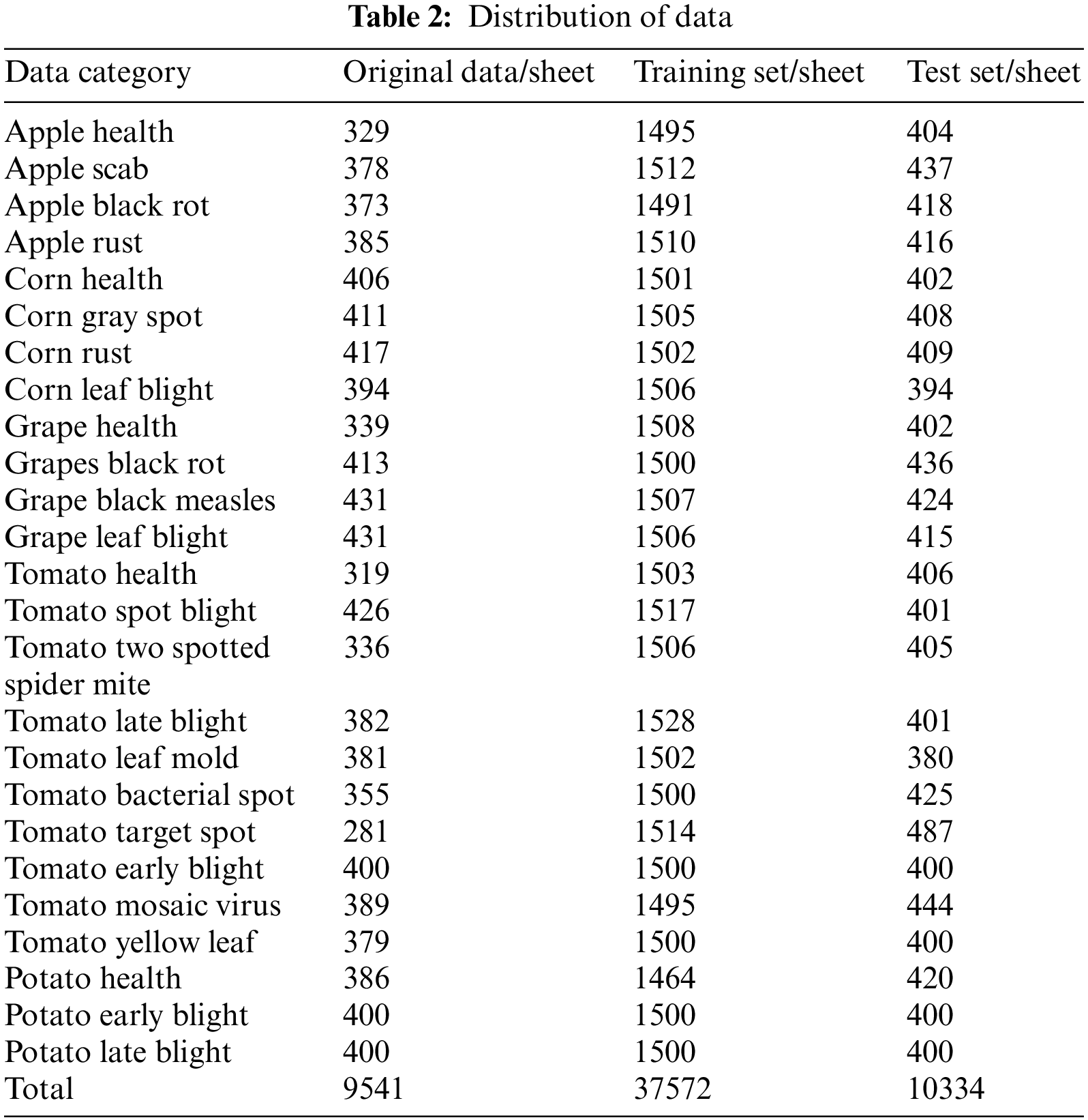
By collating the data, the problems of uneven sample distribution and low contrast are identified in the crop pest and disease leaf images. Therefore, Python is used to enhance the sample data with random horizontal/vertical flip and exposure operations. The enhancement effect is shown in Fig. 10. The final distribution of the various types of sample data after processing is shown in Table 2. The training and test sets comprise 37,572 and 10,334 images, respectively.

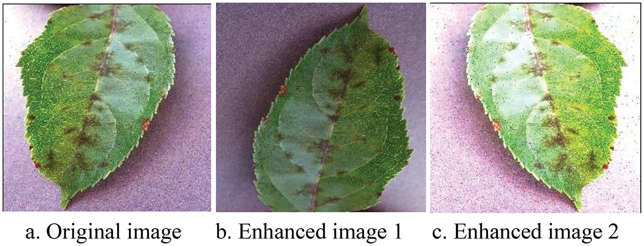
Figure 10: Example of the enhancement effect

4.3 Results

Comparison of the accuracy and loss of the proposed model with the ShuffleNetV2 model shows that the proposed model converges faster than the ShuffleNetV2 model (Fig. 11). Since the diseased leaves are photographed against a simple background, an accuracy of more than 75% is afforded at the first epoch, and the results improve by the 10th epoch of training. In the next training stage, the test accuracy further improves and the training loss further reduces. After 30 iterations, the accuracy of the proposed model is higher than that of the ShuffleNetV2 model and the loss of the proposed model is less than that of the ShuffleNetV2 model, which verifies the effectiveness of the proposed model.

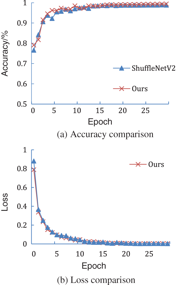
Figure 11: Comparison of the ShuffleNetV2 model and the proposed model

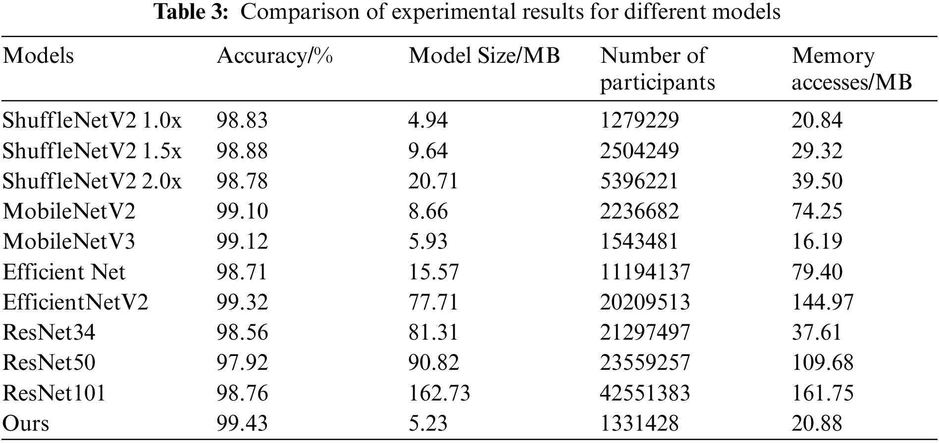
Table 3 presents the experimental results of different models. Under the same conditions, the proposed model is compared with the lightweight networks ShuffleNetV2 1.0x, ShuffleNetV2 1.5x, ShuffleNetV2 2.0x, MobileNetV2, MobileNetV3, Efficient Net, and EfficientNetV2 as well as the classical CNNs ResNet34, ResNet50, and ResNet101, further validating the effectiveness of the proposed model for crop pest and disease identification. Compared to ShuffleNetV2 1.0x, the accuracy of the proposed model is 0.6 percentage points higher and the model size is 0.29 MB greater as the MixDWConv increases the number of parameters and memory accesses by a small amount compared to the standard convolution. The proposed model exhibits better performance than ShuffleNetV2 1.5x and ShuffleNetV2 2.0x in terms of both accuracy and model size. The accuracy of the proposed model is higher than that of the lightweight networks MobileNetV2, MobileNetV3, EfficientNet, and EfficientNetV2 by 0.33, 0.31, 0.72, and 0.11 percentage points, respectively. The proposed model outperforms these four lightweight networks in terms of three metrics: model size, number of parameters, and memory access. The accuracy of the proposed model is higher than that of the classical CNNs ResNet34, ResNet50, and ResNet101 by 0.87, 1.51, and 0.67 percentage points, respectively, and it outperforms these three classical CNNs in terms of model size, number of parameters, and memory access. This shows that the proposed model exhibits the best performance in terms of recognition accuracy and model performance. Furthermore, it exhibits superior performance in identifying plant diseases and is suitable for deployment on resource-constrained mobile terminal devices.

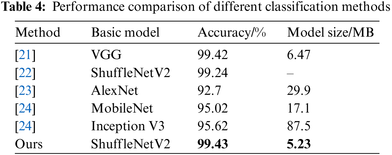
The proposed model is compared with models proposed in previous studies [21–24] that use the same PlantVillage open source dataset. The comparison results are shown in Table 4.

4.4 Ablation Study

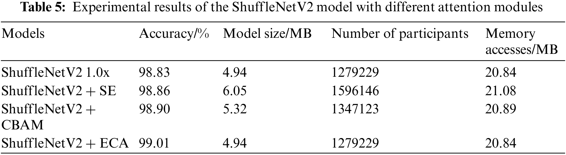
To investigate whether the introduction of the attention module is effective for identifying plant diseases, a comparative experiment is conducted. The original model of ShuffleNetV2 is compared with the ShuffleNetV2 model comprising the channel attention mechanism Squeeze-and-Excitation Networks (SE), the mixed attention module CBAM, and the ECA module. Table 5 shows that compared to the ShuffleNetV2 model, the models with SE, CBAM, and ECA modules exhibit improved recognition accuracy by 0.03, 0.07, and 0.18 percentage points, respectively. This denotes that the introduction of attention mechanisms is helpful for identifying plant diseases. Simultaneously, the experimental results show that both SE and CBAM modules increase the number of parameters and the memory access of the model, but the ECA module improves the recognition accuracy, while maintaining the light weight of the model.

To verify the effectiveness of various optimization methods in the proposed model, various optimization methods are compared with the ShuffleNetV2 1.0x model. The detailed experimental results are shown in Table 6. The incorporation of the MixDWConv, ECA module, and ReLU6 activation function on top of the ShuffleNetV2 model has a positive impact on accuracy. The addition of MixDWConv has the most significant impact on accuracy, but it also increases the model size by 0.29 MB. The addition of the ECA module and ReLU6 activation function not only affects the number of parameters of the model but also increases the recognition accuracy of the model. This demonstrates that the fusion of the ECA module and ReLU6 activation function does not adversely affect the ShuffleNetV2 network and is beneficial for improving the recognition accuracy of the model.

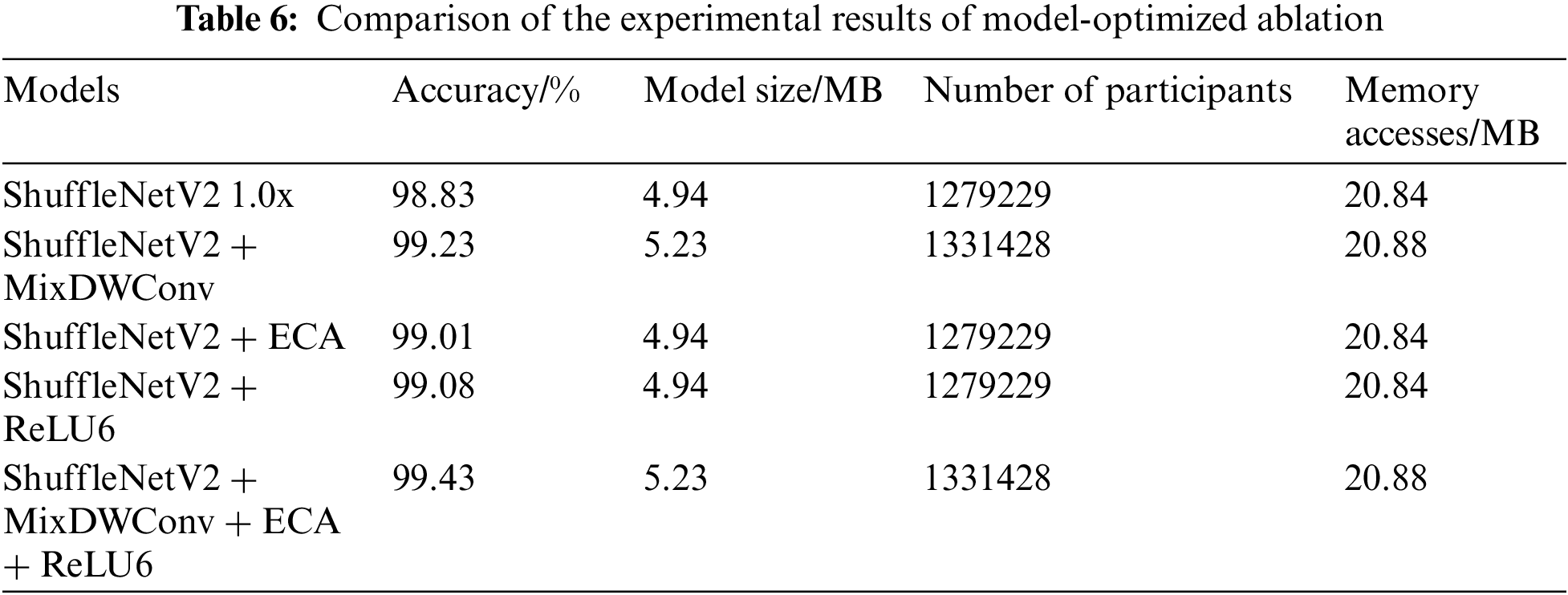
The final improved ShuffleNetV2 model incorporates MixDWConv, the ECA mechanism, and the ReLU6 activation function to achieve an optimal result. A 0.6 percentage point improvement in accuracy is achieved compared to ShuffleNetV2 1.0x, while sacrificing a small number of model parameters.

4.5 Verification of the Choice of Group Numbers for Mixed Depthwise Convolution

In this study, a lightweight model that is the modified version of ShuffleNetV2 is proposed. It uses MixDWConv in the basic module of ShuffleNetV2, i.e., all channels are divided into groups and different sizes of convolution kernels are applied to different groups. In the proposed model, g = 4 for MixDWConv. This subsection shows how different group sizes in MixDWConv influence the model performance.

Fig. 12 displays the effect of different g values in MixDWConv on the model performance. If g = 1, MixDWConv is equivalent to the ordinary depthwise convolution; thus, g is restricted from 1. As shown in Fig. 12a, the accuracy increases with the number of groups and reaches the highest value when g = 4. When g = 5, the accuracy significantly decreases. Fig. 12b displays the model loss for different g values in MixDWConv. When g = 4, the model loss is the smallest and the model exhibits the best performance. Fig. 12c shows that the model size slightly increases with the g value. Considering the three factors of model accuracy, loss, and model size, the g value with the best combined effect is selected, i.e., g = 4.

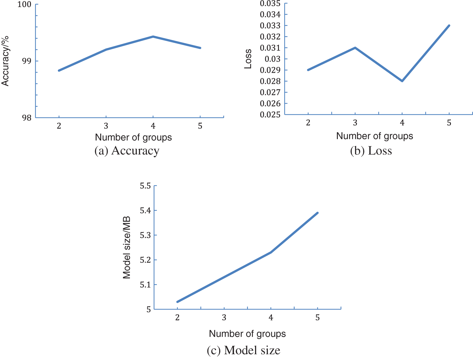
Figure 12: Effect of different numbers of groups on the model performance

5  Conclusion

To solve the problems of high complexity and large number of parameters in existing models for crop pest recognition, an improved ShuffleNetV2 crop pest recognition model was proposed. The depthwise convolution is replaced by MixDWConv, and several parameters are added to significantly improve the recognition accuracy of the model. The proposed model incorporates the ECA module to improve the model recognition accuracy without increasing the number of model parameters. The ReLU6 activation function is employed to prevent the generation of large gradients. The recognition accuracy of the proposed model on the PlantVillage public dataset is 99.43%, which makes it convenient to deploy on end devices with limited computing resources for subsequent research. Future studies will investigate methods to significantly reduce the number of parameters while maintaining the crop pest and disease recognition accuracy and comprehensively improving the model performance.

Acknowledgement: We would like to thank our professors for their instruction and our classmates for their help.

Funding Statement: This study was supported by the Guangxi Key R&D Project (Gui Ke AB21076021) and the Project of Humanities and social sciences of “cultivation plan for thousands of young and middle-aged backbone teachers in Guangxi Colleges and universities” in 2021: Research on Collaborative integration of logistics service supply chain under high-quality development goals (2021QGRW044).

Conflicts of Interest: The authors declare that they have no conflicts of interest to report regarding the present study.

References

1. Y. Q. Song, X. X. Liu and X. B. Zou, “A crop pest identification method based on a multilayer EESP deep learning model,” Journal of Agricultural Machinery, vol. 51, no. 8, pp. 196–202, 2020. [Google Scholar]

2. M. H. Wang, Z. X. Wu and Z. G. Zhou, “Research on fine-grained identification of crop pests and diseases based on attention-improved CBAM,” Journal of Agricultural Machinery, vol. 52, no. 4, pp. 239–247, 2021. [Google Scholar]

3. Z. H. Ye, M. X. Zhao and L. U. Jia, “Research on image recognition of crop diseases with complex background,” Journal of Agricultural Machinery, vol. 52, no. S1, pp. 118–124, 2021. [Google Scholar]

4. N. Krishnamoorthy, L. V. N. Prasad, C. P. Kumar, B. Subedi, H. B. Abraha et al., “Rice leaf diseases prediction using deep neural networks with transfer learning,” Environmental Research, vol. 198, no. 11, pp. 111275, 2021. [Google Scholar]

5. D. Tiwari, M. Ashish, N. Gangwar, A. Sharma, S. Patel et al., “Potato leaf diseases detection using deep learning,” in 2020 4th Int. Conf. on Intelligent Computing and Control Systems (ICICCS), Madurai, IXM, India, IEEE, pp. 461–466, 2020. [Google Scholar]

6. C. J. Wen, Q. R. Wang, H. R. Wang, J. S. Wu, J. Ni et al., “A large-scale multi-category pest identification model,” Journal of Agricultural Engineering, vol. 38, no. 8, pp. 169–177, 2022. [Google Scholar]

7. A. Krizhevsky, I. Sutskever and G. E. Hinton, “Imagenet classification with deep convolutional neural networks,” Communications of the ACM, vol. 60, no. 6, pp. 84–90, 2017. [Google Scholar]

8. K. Simonyan and A. Zisserman, “Very deep convolutional networks for large-scale image recognition,” arXiv preprint arXiv: 1409.1556, 2014. [Google Scholar]

9. K. He, X. Zhang, S. Ren and J. Sun, “Deep residual learning for image recognition,” in Proc. of the IEEE Conf. on Computer Vision and Pattern Recognition, Las Vegas, LV, USA, pp. 770–778, 2016. [Google Scholar]

10. C. Szegedy, W. Liu, Y. Jia, P. Sermanet, S. Reed et al., “Going deeper with convolutions,” in Proc. of the IEEE Conf. on Computer Vision and Pattern Recognition, Boston, USCGS-B, USA, pp. 1–9, 2015. [Google Scholar]

11. S. Bianco, R. Cadene, L. Celona and P. Napoletano, “Benchmark analysis of representative deep neural network architectures,” IEEE Access, vol. 6, pp. 64270–64277, 2018. [Google Scholar]

12. W. X. Bao, X. H. Yang, D. Liang, G. S. Hu and X. J. Yang, “Lightweight convolutional neural network model for field wheat ear disease identification,” Computers and Electronics in Agriculture, vol. 189, no. 4, pp. 106367, 2021. [Google Scholar]

13. H. Q. Hong and F. H. Huang, “Crop disease identification algorithm based on a lightweight neural network,” Journal of Shenyang Agricultural University, vol. 52, no. 2, pp. 239–245, 2021. [Google Scholar]

14. S. Q. Li, C. Chen, T. Zhu and B. Liu, “Lightweight residual network based plant leaf disease identification,” Journal of Agricultural Machinery, vol. 53, no. 3, pp. 243–250, 2022. [Google Scholar]

15. S. P. Mohanty, D. P. Hughes and M. Salathe, “Using deep learning for image-based plant disease detection,” Frontiers in Plant Science, vol. 7, pp. 1–10, 2016. [Google Scholar]

16. E. C. Too, Y. J. Liu, S. Njuki and Y. C. Liu, “A comparative study of fine-tuning deep learning models for plant disease identification,” Computers and Electronics in Agriculture, vol. 161, pp. 272–279, 2019. [Google Scholar]

17. J. Sun, W. J. Tan, H. P. Mao, X. H. Wu, Y. Chen et al., “Improved convolutional neural network-based identification of multiple plant leaf diseases,” Journal of Agricultural Engineering, vol. 33, no. 19, pp. 209–215, 2017. [Google Scholar]

18. S. F. Su, Y. Qiao and Y. Rao, “Migration learning-based identification of grape leaf diseases and mobile applications,” Journal of Agricultural Engineering, vol. 37, no. 10, pp. 127–134, 2021. [Google Scholar]

19. J. P. Xu, J. Wang, X. Xu and S. C. Ju, “Image recognition of rice fertility based on RAdam convolutional neural network,” Journal of Agricultural Engineering, vol. 37, no. 8, pp. 143–150, 2021. [Google Scholar]

20. Y. Liu and G. Q. Gao, “Identification of multiple leaf diseases using an improved SqueezeNet model,” Journal of Agricultural Engineering, vol. 37, no. 2, pp. 187–195, 2021. [Google Scholar]

21. H. M. Jia, C. B. Lang and Z. C. Jiang, “A lightweight convolutional neural network-based method for plant leaf disease identification,” Computer Applications, vol. 41, no. 6, pp. 1812–1819, 2021. [Google Scholar]

22. H. Li, W. G. Qiu and L. C. Zhang, “Improved ShuffleNet V2 for lightweight crop disease identification,” Computer Engineering and Applications, vol. 58, no. 12, pp. 260–268, 2022. [Google Scholar]

23. X. Q. Guo, T. J. Fan and X. Shu, “Image recognition of tomato leaf diseases based on improved multi-scale AlexNet,” Journal of Agricultural Engineering, vol. 35, no. 13, pp. 162–169, 2019. [Google Scholar]

24. Y. Liu, Q. Feng and S. Z. Wang, “Lightweight CNN-based plant disease identification method and mobile application,” Journal of Agricultural Engineering, vol. 35, no. 17, pp. 194–204, 2019. [Google Scholar]

25. K. Han, Y. Wang, Q. Tian, J. Guo, C. Xu et al., “Ghostnet: More features from cheap operations,” in Proc. of the IEEE/CVF Conf. on Computer Vision and Pattern Recognition, Seattle, SEA, USA, pp. 1580–1589, 2020. [Google Scholar]

26. N. Ma, X. Zhang, H. T. Zheng and J. Sun, “Shufflenet v2: Practical guidelines for efficient CNN architecture design,” in Proc. of the European Conf. on Computer Vision (ECCV), Munich, MUC, GER, pp. 116–131, 2018. [Google Scholar]

27. A. G. Howard, M. Zhu, B. Chen, D. Kalenichenko, W. Wang et al., “Mobilenets: Efficient convolutional neural networks for mobile vision applications,” arXiv preprint arXiv: 1704.04861, 2017. [Google Scholar]

28. X. Zhang, X. Zhou, M. Lin and J. Sun, “Shufflenet: An extremely efficient convolutional neural network for mobile devices,” in Proc. of the IEEE Conf.e on Computer Vision and Pattern Recognition, Salt Lake City, SLC, USA, pp. 6848–6856, 2018. [Google Scholar]

29. H. Cai, L. G. Zhu and S. Han, “Proxylessnas: Direct neural architecture search on target task and hardware,” arXiv preprint arXiv: 1812.00332, 2018. [Google Scholar]

30. M. X. Tan, B. Chen, R. M. Pang, V. Vasudevan and V. L. Quoc, “Mnasnet: Platform-aware neural architecture search for mobile,” in Proc. of the IEEE/CVF Conf. on Computer Vision and Pattern Recognition, Amoy, AM, CHN, pp. 2820–2828, 2019. [Google Scholar]

31. M. Tan and Q. V. Le, “Mixconv: Mixed depthwise convolutional kernels,” arXiv preprint arXiv:1907.09595, 2019. [Google Scholar]

32. Q. Wang, B. Wu, P. Zhu, P. Li and Q. Hu, “ECA-Net: Efficient channel attention for deep convolutional neural networks,” in Proc. of the IEEE/CVF Conf. on Computer Vision and Pattern Recognition, Seattle, SEA, USA, pp. 13–19, 2020. [Google Scholar]

33. H. X. Peng, H. J. He, Z. M. Gao, X. G. Tian, Q. T. Deng et al., “An improved ShuffleNet-V2 model-based identification method for litchi pests and diseases,” Journal of Agricultural Machinery, pp. 1–15, 2021. http://kns.cnki.net/kcms/detail/11.1964.S.20221024.1919.016.html [Google Scholar]

34. B. Liu, R. C. Jia, X. Y. Zhu, C. Yu, Z. H. Yao et al., “Mobile-oriented lightweight identification model for app-le leaf pests and diseases,” Computers, Materials & Continua, vol. 38, no. 6, pp. 130–139, 2022. [Google Scholar]

35. D. Hughes and M. Salathé, “An open access repository of images on plant health to enable the development of mobile disease diagnostics,” arXiv preprint arXiv: 1511.08060, 2015. [Google Scholar]