Stock Market Index Prediction Using Machine Learning and Deep Learning Techniques

1  Introduction

Prediction of stock market performance in terms of stock returns, closing prices, and volume traded is the most difficult activity in economic time series analysis. It is due to the unpredictable, dynamic, and nonlinear nature of stock market activities and data. The political conditions, global economic shocks, and firm financial performance add to the dynamic nature of stock market activities. Prediction of stock market returns is highly beneficial for investment decisions. Various techniques were adopted in the past few years to predict movements in stock prices. These include technical analysis and fundamental analysis methods. Trend patterns and charts are used in technical analysis based on historical price data for the identification of hidden points that may be used by investors for decision-making [1].

The fundamental analysis includes estimations based on investor moods and perceptions, financial and political news, and events that may influence the market. In recent times, advanced intelligent techniques have been used to forecast stock market performance in order to deal with nonlinear and huge-sized data. In this respect, machine learning techniques are found to be more efficient as compared to traditional methods of stock market predictions and performance analysis [2].

In addition, forecasting market returns in the stock exchange are challenging due to its nonlinear and volatile nature. Various classical algorithms and machine learning techniques are used for technical and fundamental analysis to predict market returns.

Hu et al. [3] structured a hybrid attention network (HAN) on the basis of related news patterns for predicting various trends in stock prices. Li et al. [4] are of the opinion that traditional quantitative models use time series data for predicting stock returns but these models cannot incorporate investor sentiments in such predictions. He suggested that predictions in stock returns can further be augmented by using time series along with deep learning.

The study proposed using a convolutional neural network for extracting emotional information while replacing the basic emotional characteristics of the emotional extraction level. Results suggested that this algorithm is effective and feasible for predicting variations in stock indices.

Zhong et al. [5] used artificial neural networks to predict trends in the S and P 500 index. Various dimensionality reduction techniques were used for streamlining the data set including fuzzy Robust Principal Component Analysis (FPCA), PCA, and Kernel-based Principal Component Analysis (KPCA). It was asserted that selecting an appropriate kernel function affects KPCA performance while combining PCA with Artificial Neural Networks (ANN).

Guresen et al. [6] made predictions of stock prices in NASDAQ by making a comparison among three Artificial Neural Networks (ANN) models. These ANN included dynamic artificial neural Networks (DAN2), Multilayer perception (MLP), and autoregressive conditional heteroscedasticity (GARCH). A comparison of these three models was made using mean square error (MSE) and mean absolute deviation (MAD). It was concluded that the MLP method outperformed GARCH and DAN2. Their study further recommended investigating whether GARCH has remedying impact on a stock price forecast or whether other correlated variables that have such remedial effects on a stock price forecast.

Bing et al. [7] adopted MLP and Generalized Feed Forward (GEF) to predict the market index of the Istanbul Stock Exchange. Their study made predictions using artificial neural networks and moving averages and changes the number of hidden layers. The coefficient of determination was used to measure the accuracy of predictions while the highest accuracy was achieved by using one hidden layer for both GEF and MLP.

Radial Basis Function Network (RBF) is used by Ganser et al. [8] to predict NASDAQ and Shanghai indices where Locality Preserving Projections (LPP) were used for predictions. It was asserted that the suggested method performed accurately for either of the market indices.

Rajab et al. [9] used a hybrid fuzzy logic approach for analyzing sentiments given on social media and predicting stock indices.

Sedighi et al. [10] further adopted a novel model for predicting various stock indices using ANFIS, SVM, and Artificial Bee Colony (ABC). Their study used twenty technical indices for fifty US companies as input over a period of 2008 to 2018. Quality and accuracy are taken as criteria for performance measures and concluded that this model has higher forecasting accuracy compared to others.

Deep learning techniques have become increasingly popular for stock market analysis due to their ability to capture complex non-linear relationships within large amounts of data. They can be used to identify patterns, trends, and dependencies in historical stock market data to make predictions about future stock prices. This is achieved through the use of artificial neural networks, which are capable of learning and generalizing from large amounts of data to make predictions. One of the key advantages of using deep learning techniques for stock market analysis is their ability to handle high dimensional data, such as financial data which often includes multiple features such as stock prices, trading volume, and news articles. This allows deep learning models to capture not only the historical patterns in the data but also the relationships between different features that can impact stock prices. Another advantage is the ability of deep learning models to handle time-series data, where stock prices can be considered as a sequence of values over time. This is particularly useful for stock market prediction, where historical trends and patterns in the data can be used to make predictions about future trends. Recurrent Neural Networks (RNNs) Hushani [11], such as LSTM and GRU, are particularly suited for time-series data and have been widely used for stock market prediction.

The stock market’s accurate index prediction is significantly necessary. In this work, we proposed using a recurrent neural network (RNN) to predict close prices for three stock indices. The RNNs have been observed to perform well on tasks involving sequence-based data in many research domains. With this motivation, we investigated the performance of long-short term memory (LSTM) and gated recurrent units (GRU) and their combination with stock data from three different stock indices: the KSE 100 index, the DSE 30 index, and the BSE Sensex. The results were compared to other machine learning models such as support vector regression, random forest, and k-nearest neighbor. The best results for the three datasets were obtained by the RNN-based models. The performances of the RNN-based models are higher and the proposed method could be easily incorporated into stock market index prediction.

We thus summarized our contributions in the following points:

 i)   We proposed applying three AI methods based on RNN for the task of close price predicting of three stock market indices. We also enhanced the models with the attention mechanism.

 ii)  Other machine learning techniques, including support vector regressor, random forest, and k-nearest neighbor, were also used to predict the closing prices.

iii)  The proposed RNN methods were compared with the machine learning techniques using metrics such as RMSE, explained variance, and mean gamma deviance, among others.

iv)  To measure the effect of the data range on the predictions, we conducted additional studies with a slice of the data, ignoring all instances before the year 2015.

 v)  The results displayed in the tables and figures show that our proposed RNN and attention-based methods minimized errors better and, hence, obtained the best predictions.

This work is organized as follows: Introduction is provided in Section 1. In Section 2, we explored the three datasets used. The algorithms and metrics are also explained in this section. The experimental results are discussed in Section 3. Finally, the conclusion is given in Section 4.

2  Materials and Method

2.1 Data Exploration

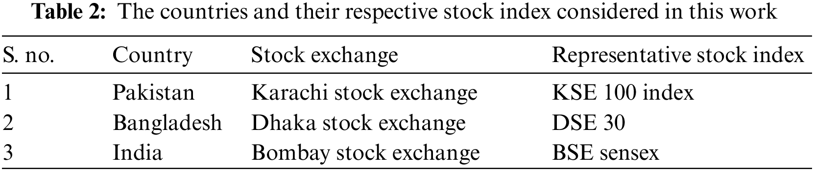
Historical data for various stock indices for this research study is collected from a website [12]. Data for three South Asian countries are collected from their major stock exchange with a major representative stock index of the country. These countries and their major stock indices are represented in Table 2. Weekly stock indices data is extracted including the weekly opening price of a relevant stock index, the opening stock index price on the given date, the highest stock index price on the given date, the lowest stock index price on the given date, the volume of shares traded on the given date and weekly percentage change in the stock price index. The Stock Return (SR) in the last column of the table is calculated by subtracting the Previous week’s price of the stock index (SI) from the current week’s price and dividing by the current week’s price, as shown in Eq. (1):

SR=WeeknSI−Week(n−1)SIWeek(n−1)SI×100(1)

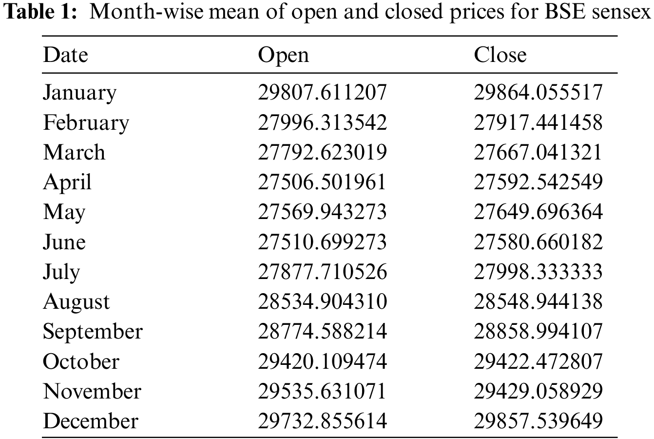
2.1.1 Bombay Stock Exchange (BSE)

This data was gathered for the period 2009-05-31 to 2022-01-23, making a total of 4620 days. The mean for each month of this period is shown in Table 1. The lowest monthly mean for the open price is 27,506.50, recorded in April. The highest open price means is 29,807.61 recorded in January. Likewise, the lowest mean closing price is 27,998.33, recorded in June, while the highest mean closing price is 29,864.05, recorded in January.

The low and high stock prices for BSE are also explored to identify the highest and lowest recordings based on the month, as shown in Fig. 1a. For the high stock prices, the highest value of 61,475.15 was recorded in January, and the lowest value of 50372.23 in April, as shown by the figure.

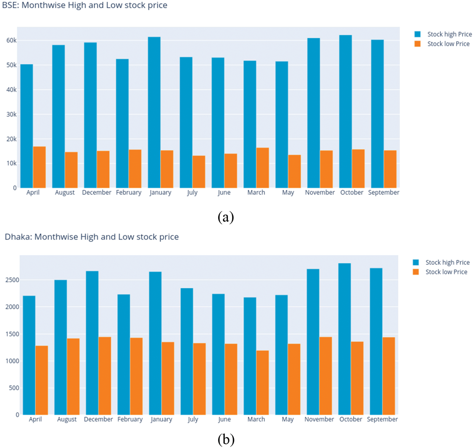
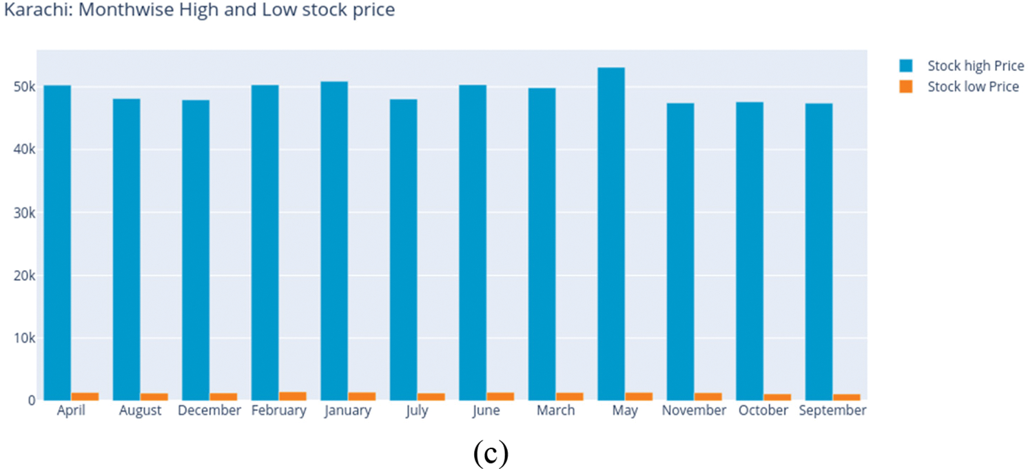
Figure 1: Month-wise high and low prices for (a) BSE, (b) DSE, and (c) KSE

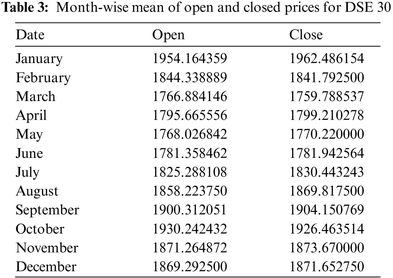
2.1.2 Dhaka Stock Exchange (DSE)

The data collected for DSE covers the period 2013-02-03 to 2022-01-23, making a total of 3276 days. The mean for each month of this period is shown in Table 3. The lowest monthly mean for the open price is 1,766.88, recorded in the month of March. The highest open price means is 1,954.16 recorded in January. Likewise, the lowest mean closing price is 1,759.80, recorded in March, while the highest mean closing price is 1,962.49, recorded in January. The low and high stock prices for DSE are also explored to identify the highest and lowest recordings based on the month, as shown in Fig. 1b. For the high stock prices, the highest value of 2,807.80 was recorded in October, and the lowest value of 2174.98 in March, as shown by the figure.

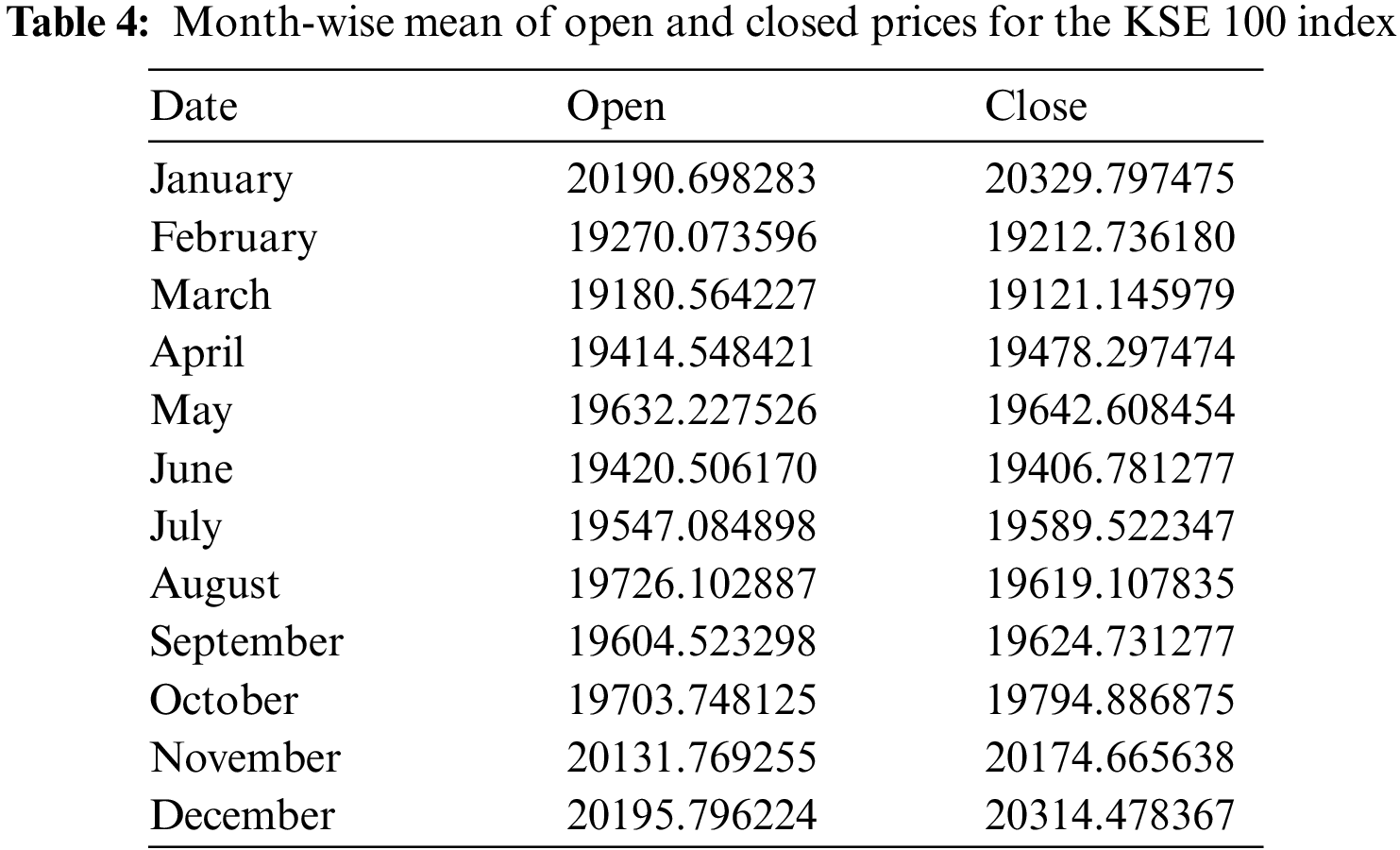
2.1.3 Karachi Stock Exchange (KSE)

The data collected for KSE begins from 2000-01-09 and ends at 2022-01-16 accounting for 8043 days. Table 4 contains the averages of open and close prices for the months. The lowest month-wise means for the open and close prices are 19,180.56 and 19,121.15 respectively, observed in March. However, the highest mean open price, 20,195.80 is observed in December, while the highest mean close price, 20,329.80 is observed in January regarding the stock prices for KSE, see Fig. 1c. The largest occurred high price is 53,127.24 in the month of May, while the lowest is 47,387.34, occurring in September. Also, the low price is highest in February at 1,415.51 and lowest in September at 1,069.55.

2.2 Algorithms

We investigated the performance of several machine learning algorithms with each of the different sources of data. Aside from the typical ML methods, we also used two deep-learning methods popularly used on sequential data; LSTM and GRU, a combination of these two methods, and their attention-based enhancements. We describe the algorithms as follows:

2.2.1 Support Vector Regressor (SVR)

An approach for supervised learning called support vector regression is used for predicting discrete values. The SVMs and Support Vector Regression both operate on the same theory. Finding the optimum fit line is the fundamental tenet of SVR. The hyperplane with the most points is the best-fitting line in SVR. The SVR seeks to match the best line within a threshold value, in contrast to other regression models that aim to reduce the error between the true and their predictions. The distance between the boundary line and the hyperplane is the threshold value. SVR is difficult to scale to datasets with more than a few ten thousand samples since the fit time complexity is more than quadratic with the number of samples. In our implementation, the radial basis function was used as the kernel. The gamma value is set to 0.1, and the regularization parameter, C is set to 1e2.

2.2.2 Random Forest Regressor (RF)

Decision trees (DT) are one of the most popular classifiers used in machine learning. A decision tree is a decision-making tool that employs a tree-like framework of choices and their possible results, such as chance event outcomes, resource costs, and utility. One way to approach it is to illustrate an algorithm with conditional control statements. DTs are usually designed as flow diagrams made up of the root nodes, the internal nodes, and the leaf nodes. A decision tree begins with a root node that is not formed by incoming branches. The branches from the root nodes are fed to the internal nodes for decision-making. These nodes evaluate the given features to generate homogeneous subsets that are indicated by leaf nodes or end nodes. The end nodes represent all the dataset’s conceivable outcomes. Random forest is simply an ensemble of decision trees, and they can either be used for classification; where the output is the class selected by most of the trees, or for regression problems, where the output is the mean of the results of the decision trees.

Scikit Learn library was used for our implementation. The random forest contains a total of 100 decision trees with the “squared error” criterion. The maximum depth of the trees is set to “none” which means that the trees will continue to grow until all the leaves are pure or until the leaves contain less than “min samples split” samples. The number of features to be considered for splitting a node is determined by the parameter “max features” set to “auto”. The minimum number of samples required to split an internal node and the minimum number of samples required to be a leaf node are set to 2 and 1 respectively. The implementation also has a random state of 0 and is not set to use out-of-bag samples.

2.2.3 K-Nearest Neighbour (K-NN)

K-NN is a supervised learning technique that is non-parametric. It can be used for either regression or classification tasks. The k closest training samples of the data are fed as input and the result when performing classification is a class membership. An object is allocated to the class most frequently chosen by its k closest neighbors based on a majority vote among the item’s neighbors. When using k-NN for regression, the output is the object’s property value, which is obtained by taking the average of the values of the k closest neighbors. The k value in our experiments for the three datasets was set to 15.

2.3 RNN-Based Models

A recurrent neural network (RNN) is a type of artificial neural network in which node connectivity can form a loop, enabling outputs from one node to influence future inputs to the very same node. This enables it to display temporal dynamic characteristics. RNNs, which are based on feedforward neural networks, can analyze input sequences of variable length using the internal state (memory). As a result, they can be used for tasks like handwriting or speech recognition. RNNs can be distinguished from convolutional neural networks (CNNs) in that RNNs are networked with infinite impulse responses, while CNNs are networking with finite impulse responses. Both types of networks display temporal dynamics.

An infinite impulse recurrent network is a directed cyclic graph that cannot be unrolled and substituted with a complete feedforward neural network, whereas a finite impulse recurrent network can be unrolled. The inputs and outputs of RNNs can vary in length so that configurations such as one-to-one, one-to-many, many-to-one, and many-to-many are possible. Like in CNNs, activation functions such as Sigmoid, Tanh, and Relu can be used in RNNs. This paper experiments with two of the variants of RNN: long short-term memory (LSTM) and gated recurrent units (GRU).

2.3.1 Long-Short-Term Memory (LSTM)

LSTM [13–15] is proposed to extend the recurrent neural network in capturing information in both the long-term and short-term. Long-term memory can be compared to the way changes in synaptic strengths keep memories for the long term. In a similar fashion, for a network, the weights and biases are changed once for every training episode.

To keep short-term memory, the activations are updated every time step, which is also similar to the way short-term memory is stored in the brain as a result of moment-to-moment changes in the pattern of the electrical firings. We constructed the LSTM network with the Keras sequential module. First, an LSTM layer with 32 internal units is added, and we set the return sequences argument to true. The input shape argument was set to (15,1). The second LSTM layer is added, again with 32 internal units, and the return sequence is set to true. Finally, we added the last LSTM layer with 32 internal units whose output is transferred to a dense layer. We used the mean squared error as the loss function and Adam as the optimizer. Each of the datasets was split into train-test sets, and training was carried out for 200 epochs.

2.3.2 Gated Recurrent Unit (GRU)

Another common recurrent neural network method is the GRU [16]. The GRU is similar to the LSTM but has a forget gate and fewer parameters than the LSTM. The GRU is constructed in a similar configuration as the LSTM network. The first GRU layer consists of 32 internal units with the return sequences argument set to true and the input shape arguments set to (15, 1).

The second GRU layer also consists of 32 internal units with the return sequence argument set to true. Finally, the last LSTM layer consists of 32 internal units whose output is transferred to a dense layer. The mean squared error was used to compute the loss, and the Adam optimizer was used. The training set was trained for 200 epochs.

2.3.3 LSTM + GRU

A hybrid model involving LSTM and GRU was designed by stacking these two methods. We composed this model with two LSTM layers followed by two GRU layers and then a dense layer. In detail, the first LSTM consists of 32 internal units with the return sequences set to true and the input shape set to 15.

Another LSTM layer of 32 internal units was added. We again returned the sequences as input to the third recurrent layer. This third layer is a GRU with 35 internal units. The sequences are again returned to the last GRU layer with 32 internal units. The final layer is a dense layer. We used the mean squared error as our loss function and Adam as the optimizer. We also trained this model for 200 epochs.

2.4 Attention Mechanism

In recent years, the attention mechanism has gained popularity in various natural language processing tasks such as machine translation and text summarization. The attention mechanism allows the model to focus on certain parts of the input while disregarding irrelevant information.

In this paper, we explore the use of the attention mechanism in time series forecasting. The attention mechanism is incorporated into the RNN models described previously.

2.4.1 LSTM or GRU with Attention

We begin by reshaping the input to have the shape (samples, time steps, features) which is required for LSTM/GRU. The LSTM/GRU layer has 32 units and returns sequences to be used as input for the attention mechanism. The attention mechanism is implemented using the Dot product method, where the dot product of the query and key tensors is taken and used to calculate the attention weights. These attention weights are then multiplied with the value tensor to get the attention output. The attention output is concatenated with the LSTM/GRU output. This merged output becomes an input to a second LSTM/GRU layer with another 32 units. The attention is again implemented and the weights are concatenated with the output of the LSTM/GRU layer. A final LSTM/GRU layer with 32 units takes the results. Now the return sequences argument is set to false. The output from this last layer is passed to the dense layer for prediction.

2.4.2 LSTM-GRU with Attention

Finally, we combine the LSTM and GRU models with the attention mechanism to create an LSTM-GRU model. Similarly to the previous description, the input is reshaped to have the shape (samples, time steps, features) which is required for both LSTM and GRU. The first two layers of the model are the LSTM layers with 32 units each and the return sequences options set to True. The attention mechanism is implemented in the same way explained previously; using the Dot product method, where the dot product of the query and key tensors is taken and used to calculate the attention weights. These attention weights are then multiplied with the value tensor to get the attention output. The attention output is concatenated with the second LSTM output and a third and fourth layers are added which are GRU layers with 32 units each. Another attention is computed and its output is concatenated with the output of the GRU layer before forwarding to the dense layer for the prediction.

2.5 Steps

The overall architectures of the proposed RNN-based models are presented in Fig. 2. For each of the networks, namely; LSTM, GRU, and LSTM + GRU, and their attention-based variations, the following steps were performed:

Figure 2: Proposed flow for prediction with LSTM, GRU, LSTM + GRU, LSTM + Attention, GRU + Attention, and LSTM + GRU + Attention models

Step 1: The data corresponding to BSE, DSE, and KSE were explored, and the closing prices were reshaped into samples, time steps, and features as required by RNN-based models.

Step 2: The data is then passed through the networks. Three layers of LSTM layers are followed by a dense layer for the LSTM model. Likewise, for the GRU model, three layers of the GRU are stacked and followed by a dense layer. For the LSTM + GRU model, two GRU layers were stacked on two LSTM layers, followed by the dense layer. For the attention-based variations for LSTM and GRU, we added computed the attention twice. One after the first LSTM/GRU layer and again after the second LSTM/GRU layer. For the hybrid model, LSTM + GRU + Att, we computed the attention twice, the first after the two LSTM layers and the second after the two GRU layers.

Step 3: The predictions obtained from each of the models were used with the original closing prices to compute the evaluation metrics.

2.6 Evaluation Metrics

Model evaluation is a crucial aspect of every research. In measuring the performance of the various methods used, we adopted the following evaluation metrics: mean square error (MSE), root mean square error (RMSE), mean absolute error (MAE), explained variance regression score, R2 score), mean gamma deviance regression loss (MGD), and mean Poisson deviance regression loss (MPD) for both the training data set and the testing data set.

3  Experimental Results and Discussion

The original data on the close prices and the predictions for all the stock indices are shown in Fig. 3. The following explains the results obtained on the various metrics.

Figure 3: Comparing the original close prices and the predicted close prices for (a) BSE, (b) Dhaka, and (c) Karachi

3.1 BSE

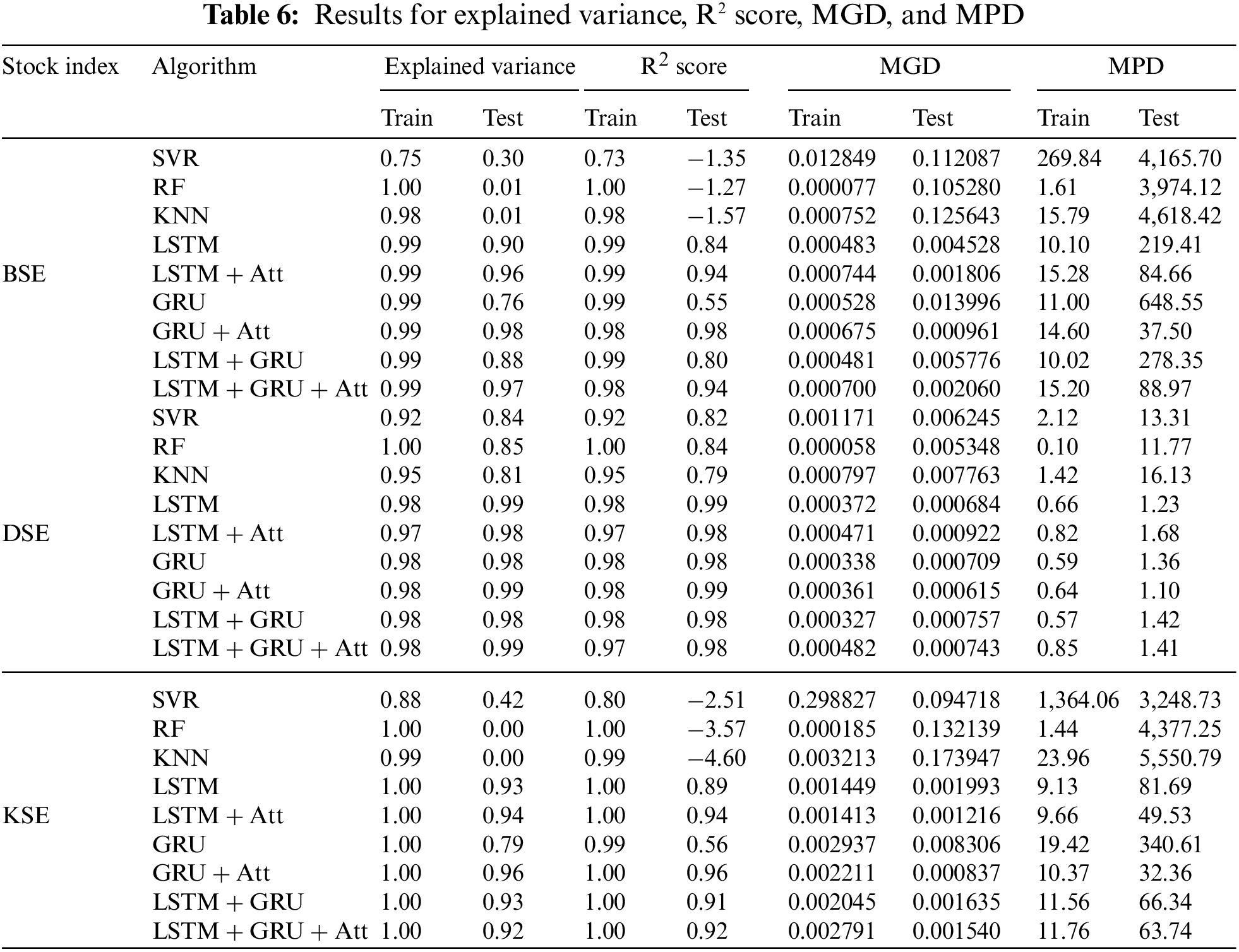
The results, as presented in Tables 5 and 6, show that the GRU + Att algorithm per- formed the best overall, with the lowest RMSE, MSE, MAE, MGD, and MPD and the highest explained variance, R2 score on the test set. This suggests that the GRU + Att algorithm is able to provide the most accurate and consistent predictions for the BSE index.

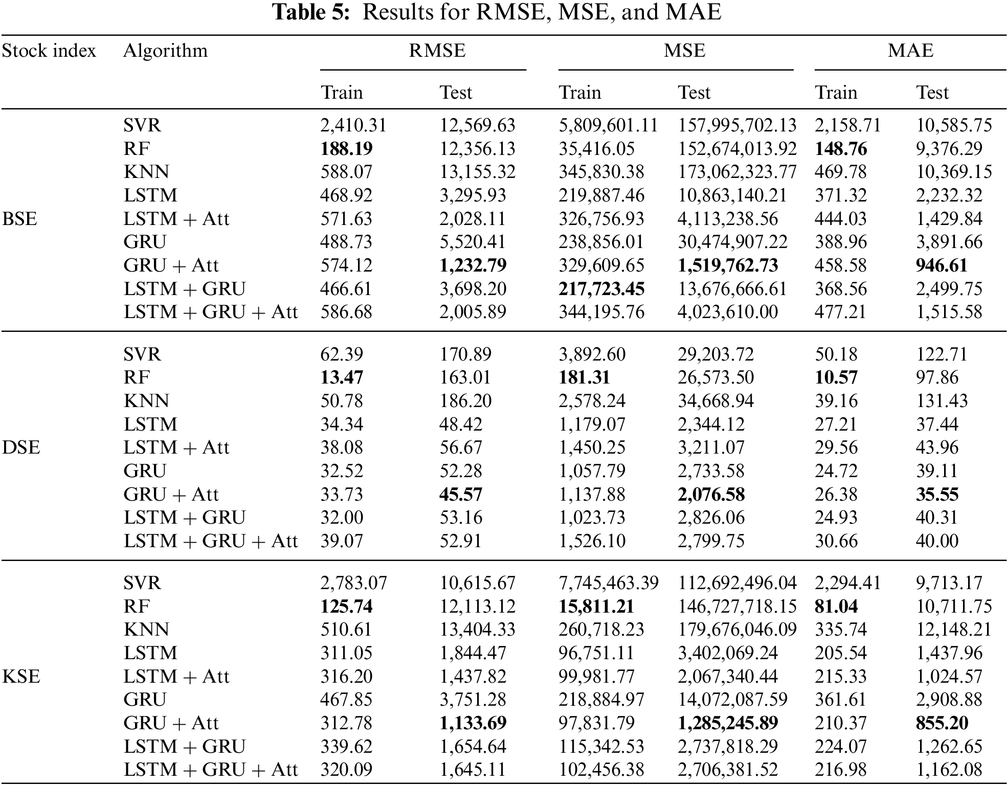
On the other hand, the SVR algorithm performed the worst, with the highest RMSE, MSE, and MAE, and the lowest explained variance, R2 score. SVR also attained too high values for MGD and MPD on the test set. This suggests that the SVR algorithm is not well suited for the task of stock index prediction.

It is worth noting that the LSTM, LSTM + Att, GRU, LSTM+GRU, and LSTM + GRU + Att algorithms all performed relatively well, with RMSE, MSE, MAE, and R2 score values that were close to those of the GRU + Att algorithm. However, these algorithms did not perform as well in terms of explained variance, MGD, and MPD. From the results, the GRU + Att algorithm is the best choice for stock index prediction when considering the BSE. However, the other algorithms, LSTM, LSTM + Att, GRU, LSTM + GRU, and LSTM + GRU + Att are also good options, as they have similar performance in terms of RMSE, MSE, MAE, and R2 score, but not as well in terms of explained variance, MGD, and MPD.

3.2 DSE

Also for the DSE, the results in Tables 5 and 6 that the GRU + Att model performs the best in terms of RMSE, MSE, MAE, explained variance, and R-squared score, with the lowest values for these metrics. This was followed by the LSTM model, indicating that these models are able to make more accurate predictions on the DSE stock index compared to the other algorithms. The GRU + Att and the LSTM models have RMSE of 45.57 and 48.42 respectively, which are significantly lower than the other models, and both have R-squared scores of 0.99, which is the highest among all the models.

It is also worth noting that the GRU + Att and LSTM models have the lowest MGD and MPD values. This suggests that these models have the smallest deviation from the actual stock prices and are able to predict stock prices with high accuracy.

On the other hand, the SVR and KNN models perform poorly in comparison, with high RMSE, MSE, MAE, MGD, and MPD values. The SVR model has an RMSE of 170.89, which is the highest among all the models, and an R-squared score of 0.84. The KNN model also has a high RMSE of 186.20 and an R-squared score of 0.79. The RF performed better than the SVR and KNN models but its performance is worse than the RNN-based models.

The GRU, LSTM + ATT, LSTM + GRU, and LSTM + GRU + Att models perform similarly to LSTM, GRU + Att models, with slightly higher RMSE, MSE, MAE and slightly lower R-squared score, explained variance, MGD, and MPD values.

In conclusion, the GRU + Att and LSTM models have the best performance in terms of accuracy in predicting the DSE stock index, followed by the GRU model, LSTM + GRU + Att model, LSTM + GRU model, and RF model, while the SVR and KNN models show the worst performance. The use of attention mechanisms in GRU models has been shown to have slightly improved performance. Based on these results, it can be recommended to use GRU + Att or LSTM models for stock price prediction on the DSE index.

3.3 KSE

It can be seen that the LSTM + Att and GRU + Att models performed the best in terms of RMSE and MAE, with the lowest values for the test set. These models also had the highest explained variance and R-squared scores, indicating that they were able to accurately capture the underlying trends in the data. The LSTM + mAtt and GRU + Att models also had the lowest values for MGD and MPD, indicating that they had the smallest deviation from the true values.

On the other hand, the SVR model performed the worst in terms of all the evaluation metrics. The RF and KNN models performed slightly better than the SVR model, but still had relatively high values for RMSE, MSE, and MAE. The GRU, LSTM, GRU, and LSTM + GRU + Att models performed similarly to the LSTM + Att and GRU + Att models in terms of RMSE and MAE but had slightly lower explained variance and R-squared scores. Hence, the LSTM + Att and GRU + Att models performed the best for stock index prediction on the KSE dataset.

These models were able to capture the underlying trends in the data and had the smallest deviation from the true values. The SVR model performed the worst, while the RF and KNN models had relatively high errors. The LSTM, GRU, LSTM + GRU, and LSTM + GRU + Att models performed similarly to the LSTM and LSTM + Att models, but with slightly lower explained variance and R-squared scores.

3.4 Using Slices of the BSE, DSE, and KSE Data

Tables 7 and 8 and Fig. 4 are the results obtained when we only used data with closing prices above 2014. From Table 7, the GRU + Att model obtained the best results on the RMSE, MSE and MAE for the BSE index. The LSTM + GRU + Att model also performed close to the GRU + Att model on the metrics for the same BSE index. Considering the DSE index, the GRU + Att model again got the lowest RMSE of 52.86, which is closely followed by the LSTM + GRU model with 58.71 and then the GRU model with 60.40 and the LSTM and LSTM + GRU + Att with 80.02 and 85.45 respectively on the test data. Again for the DSE, the lowest values for the MSE and MAE metrics were obtained by the GRU + Att model. Similar results were obtained on the KSE index where the GRU and GRU + Att models performed best on the RMSE. The MSE metrics. For the MAE, the GRU + Att had the lowest value while the LSTM + Att, the GRU, and the LSTM + GRU + Att were around the same values. The SVR and the KNN performed worst in this case.

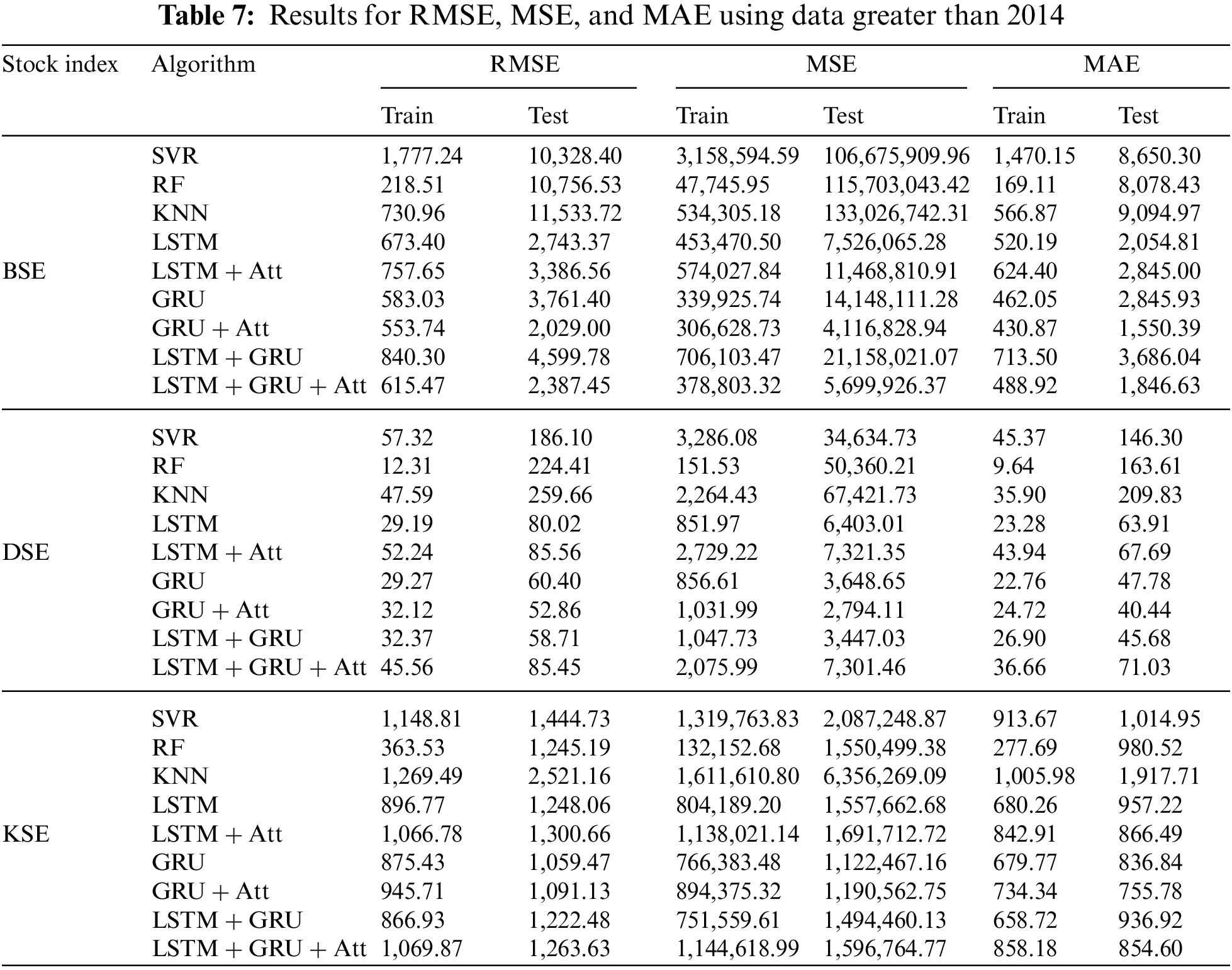
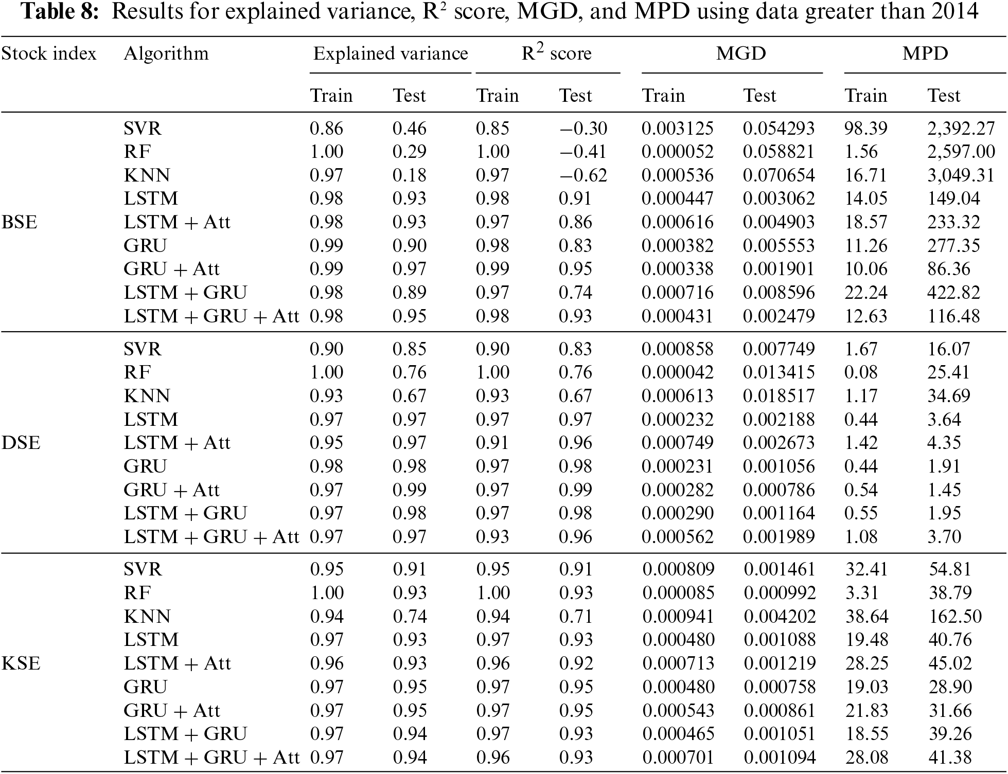
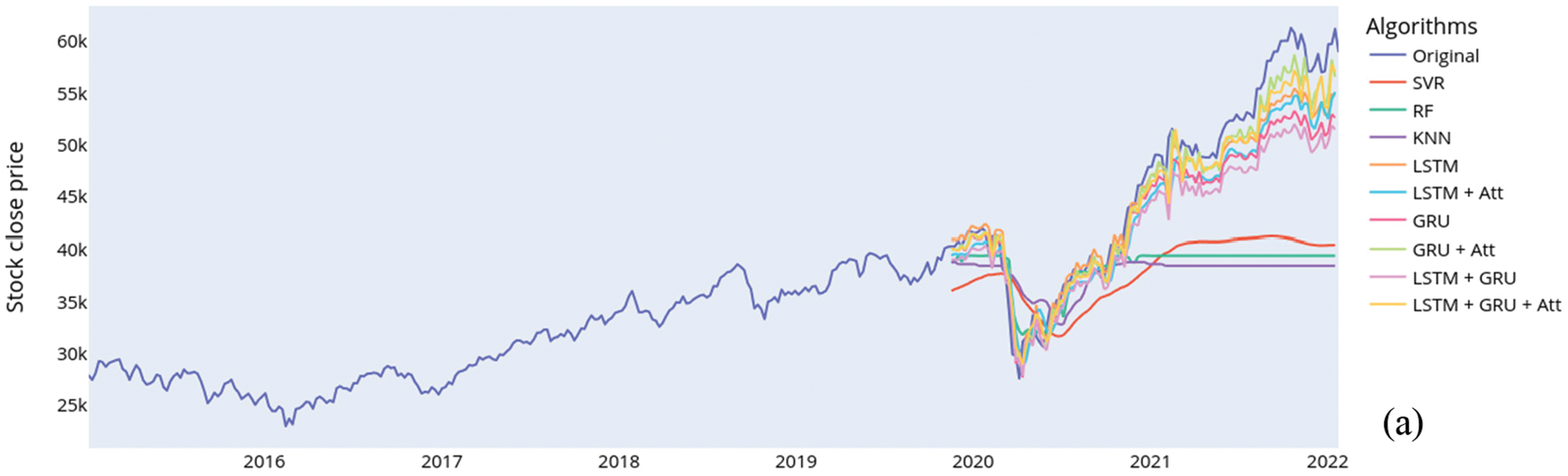
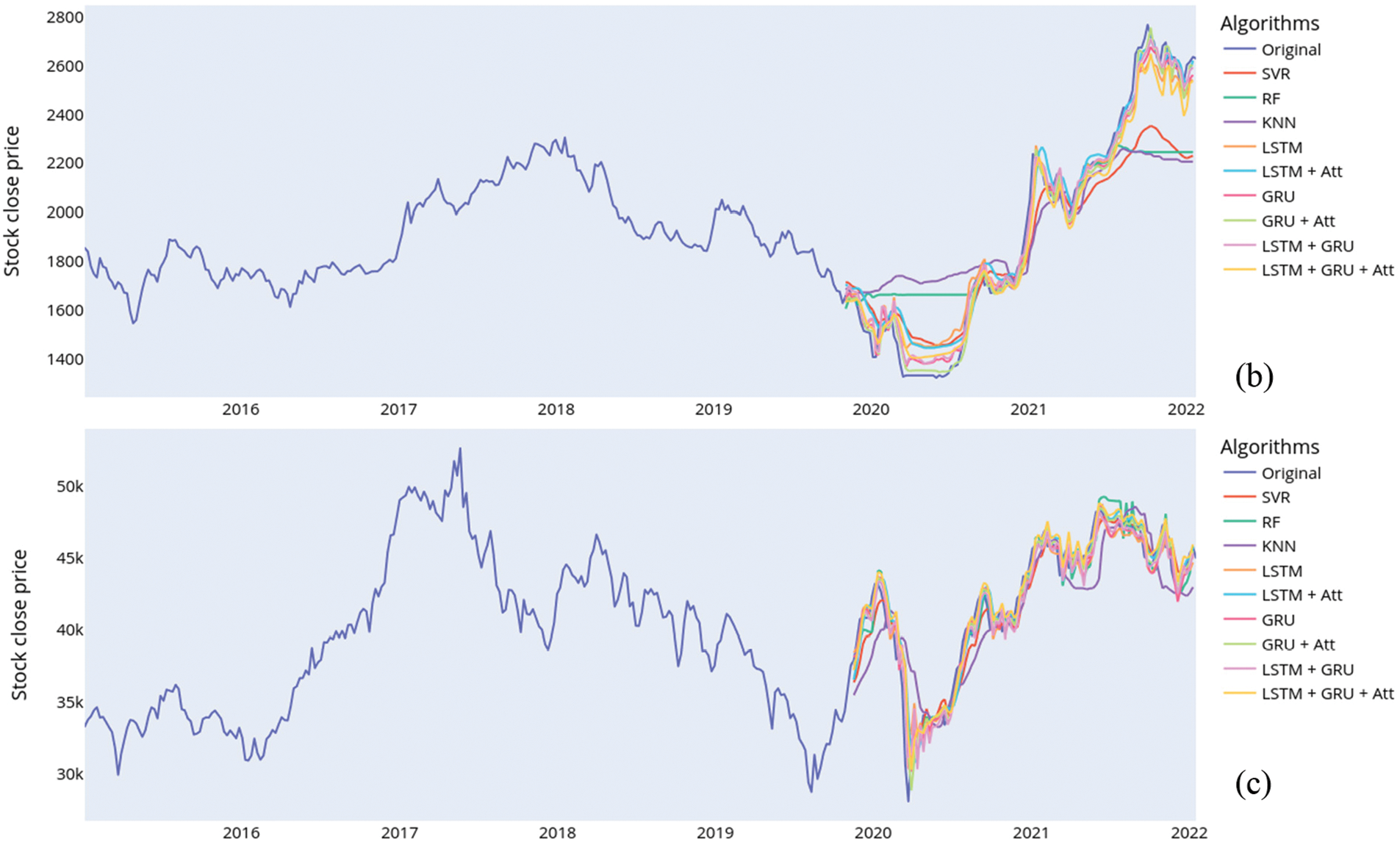
Figure 4: Using a slice of the data above the year 2014 for the experiment, the sub-figures compare the original close prices and the predicted close prices for (a) BSE, (b) Dhaka, and (c) Karachi

Table 8 presents the results for the three indices on the explained variance, the R2 score,

the MGD and the MPD. Considering the BSE index, the GRU + Att model had an explained variance of 0.97 followed by the LSTM + GRU + Att with 0.95. The other RNN models also performed much better on the RMSE than the SVR, RF, and KNN for the BSE test data. For the DSE index, the highest explained variance and R2 of 0.99 on the test data were obtained by the GRU + Att model. The lowest MGD and MPD values were again obtained by the GRU + Att model making it the best model for DSE. The other RNN models and their attention-based variations also outperformed the SVR, RF, and KNN. Lastly, considering the KSE, the GRU and GRU + Att models had the highest variance of 0.95 and R2 score of 0.95 On the test data. This is followed by the LSTM + GRU and LSTM + GRU + Att with 0.94 And 0.93 respectively. Adding attention to the LSTM however, did not improve the LSTM on the KSE data. Likewise, the attention does not improve the MGD and MPD for the GRU and the LSTM + GRU models.

Though using the entire dataset allows the models to better capture long-term trends in the stock market, using a more recent slice of the data enables the models to learn to become better suited to predicting current market trends.

4  Conclusion

Predicting the stock market is an interesting research area for both economists and computer scientists. Classical machine learning techniques have been used in much of the literature for predictions, but recent advances in RNN have proven to be very effective with sequence-based data in several research domains. In this study, we evaluated the performance of RNN-based models, including Long-Short Term Memory (LSTM), Gated Recurrent Unit (GRU), and a hybrid model of LSTM and GRU, in time series forecasting;

Predicting the closing prices of three stock indices, namely the KSE 100 index, the DSE 30, and the BSE Sensex. We also explored the use of attention mechanisms in these models to improve their performance. Lastly, traditional machine learning models namely SVR, RF, and KNN were used as baseline models. Our results showed that the hybrid model of LSTM and GRU outperformed the single models of LSTM and GRU. The attention mechanism was also found to be effective in improving the performance of these models. SVR, RF, and KNN models obtained the worst performances on our data.

Overall, our study highlights the effectiveness of RNN-based models and the attention mechanism in time series forecasting. These models provide an effective solution for tasks that require the analysis of input sequences of variable length and temporal dynamic characteristics.

This work provides a basis for further studies on the use of RNNs and attention mechanisms in time series forecasting. Other deep learning techniques such as transfer learning, data augmentation, etc. for time series predictions are also worth studying in the future. Whiles this paper only focused on using historical stock prices and trends. Other factors including economic indicators such as gross domestic product (GDP), inflation, and interest rates do affect future trends and hence further studies are required.

Acknowledgement: This research work was carried out as a joint research collaboration at the University of Electronic Science and Technology of China, Chengdu China, Yangtze Delta Region Institute (Huzhou), University of Electronic Science and Technology of China, Huzhou, 313001, China, and Adbul wali khan Mardan KPK, Pakistan and Brain Institute Peshawar, Peshawar, 25130, Pakistan. The authors are thankful for this support. The Cobbinah Bernard Mawuli supporting in the proofreading of the revised manuscript.

Funding Statement: This research work is supported by NRPU Project No. 20-16091awarded by Higher Education Commission, Pakistan. The title of the project is “University Education and Occupational Skills Mismatch (A Case Study of SMEs in Khyber Pakhtunkhwa)”, by the National Natural Science Foundation of China (Grant No. 61370073), the National High Technology Research and Development Program of China, the project of Science and Technology Department of Sichuan Province (Grant No. 2021YFG0322).

Author Contributions: Conceptualization, A.U.H., and A.H.; B.L.Y.A, J.P.L, and A.S methodology, A.U.H., and B.L.Y.A., A.S, software, A.U.H.; validation, A.U.H., and A.H.; A.H.U, formal analysis, A.U.H., R.K, and B.L.Y.A.; investigation, A.U.H., J. P. L, and A.S., resources, A.U.H., and B.L.Y.A., and A.S A; writing–original draft preparation, A.U.H.; writing–review and editing, B.L.Y.A., A.U.H; visualization, A.U.H.; supervision, A.H.; J.P.L, and A.S project administration, A.U.H.; funding acquisition, R.K, and A.H. All authors have read and agreed to the published version of the manuscript.

Availability of Data and Materials: Data for this study is extracted from investing.com, URL: (https://www.investing.com/indice indices & major India additional Indices) and can be made available upon request. The corresponding author Amin ul Haq (http://khan.amin50@yahoo.com) would be contacted for data availability.

Ethics Approval: This article does not contain any studies with human participants or animals performed by any of the authors.

Conflicts of Interest: The authors declare that they have no conflicts of interest to report regarding the present study.

References

1. R. Halil and M. Demirci, “Predicting the turkish stock market bist 30 index using deep learning,” International Journal of Engineering Research and Development, vol. 11, no. 1, pp. 253–265, 2019. [Google Scholar]

2. L. Li, Y. Wu, Y. Ou, Q. Li, Y. Zhou et al., “Research on machine learning algorithms and feature extraction for time series,” in 2017 IEEE 28th Annual Int. Symp. on Personal, Indoor, and Mobile Radio Communications (PIMRC), Montreal, M, Canada, pp. 1–5, 2017. [Google Scholar]

3. Z. Hu, W. Liu, J. Bian, X. Liu and T. Liu, “Listening to chaotic whispers: A deep learning framework for news-oriented stock trend prediction,” in Proc. of the Eleventh ACM Int. Conf. on Web Search and Data Mining, New York, NY, USA, pp. 261–269, 2018. [Google Scholar]

4. J. Li, “Research on market stock index prediction based on network security and deep learning,” Security and Communication Networks, vol. 2021, no. 1, pp. 1–8, 2021. [Google Scholar]

5. X. Zhong and D. Enke, “Forecasting daily stock market return using dimensionality reduction,” Expert Systems with Applications, vol. 67, no. 1, pp. 126–139, 2017. [Google Scholar]

6. E. Guresen, G. Kayakutlu and T. U. Daim, “Using artificial neural network models in stock market index prediction,” Expert Systems with Applications, vol. 38, no. 8, pp. 10389–10397, 2011. [Google Scholar]

7. Y. Bing, J. K. Hao and S. C. Zhang, “Stock market prediction using artificial neural networks,” in Advanced Engineering Forum, vol. 6, Switzerland: Trans Tech Publications, pp. 1055–1060, 2012. [Google Scholar]

8. A. Ganser, B. Hollaus and S. Stabinger, “Classification of tennis shot with a neural network approach,” Sensors, vol. 21, no. 17, pp. 5703, 2021. [Google Scholar] [PubMed]

9. S. Rajab and V. Sharma, “An interpretable neuro-fuzzy approach to stock price forecasting,” Soft Computing, vol. 23, no. 3, pp. 921–936, 2019. [Google Scholar]

10. M. Sedighi, H. Jahangirnia, M. Gharakhani and S. F. Fard, “A novel hybrid model for stock price forecasting based on metaheuristics and support vector machine,” Data, vol. 4, no. 2, pp. 75, 2019. [Google Scholar]

11. P. Hushani, “Using autoregressive modelling and machine learning for stock market prediction and trading,” in Third International Congress on Information and Communication Technology. London, L: UK, pp. 767–774, 2019. [Google Scholar]

12. Investing.com, Stock market quotes & financial news. Investing.com, 2023. [Online]. Available: https://www.investing.com [Google Scholar]

13. A. U. Haq, J. P. Li, B. L. Y. Agbley, C. B. Mawuli, Z. Ali et al., “A survey of deep learning techniques based Parkinson’s disease recognition methods employing clinical data,” Expert Systems with Applications, vol. 208, no. 3, pp. 118045, 2022. [Google Scholar]

14. A. U. Haq, J. P. Li, Z. Ali, I. Khan, A. Khan et al., “Stacking approach for accurate invasive ductal carcinoma classification,” Computers and Electrical Engineering, vol. 100, no. 3, pp. 107937, 2022. [Google Scholar]

15. U. D. Maiwada, “Introductory technology as it impacts modern society in the world,” Journal of Technology Innovations and Energy, vol. 1, no. 1, pp. 36–42, 2022. [Google Scholar]

16. A. U. Haq, J. P. Li, B. L. Y. Agbley, A. Khan, I. Khan et al., “IIMFCBM: Intelligent integrated model for feature extraction and classification of brain tumors using MRI clinical imaging data in IoT-healthcare,” IEEE Journal of Biomedical and Health Informatics, vol. 26, no. 10, pp. 5004–5012, 2022. [Google Scholar] [PubMed]