Missing Value Imputation Model Based on Adversarial Autoencoder Using Spatiotemporal Feature Extraction

1  Introduction

A lot of data is being generated due to the internet of things and sensors, the increase in tracking and collection of customer data by enterprises, the increase in unstructured data caused by the spread of social network services, the development of storage media technology and the fall in prices. Currently, there is active research on big data, Artificial Intelligence (AI), machine learning, and deep learning, in which data plays a key role among the representative technologies of the 4th industrial revolution [1–3]. In such studies, the performance of the model is determined by the quantity and quality of the data, but the quantitative aspect of the data is being resolved, but the quality of the data is inferior because there are many cases where values are missing or strange values are stored for a series of reasons (e.g., malfunction of equipment, refusal to respond to surveys, etc.) in the collection process in reality. This leads to difficulties in data analysis, an unbalanced data structure, and a decrease in the predictive performance of the model [4,5]. Therefore, research through the application of algorithms and statistical methods to impute missing values is actively underway. There are statistical methods that remove missing values or impute them with mean, median, and mode, and alternative methods that utilize k-recent neighbor search, a machine learning algorithm. In the case of these methods, however, if the proportion of data including missing values is small compared to the size of the entire data, which will affect statistical analysis results and algorithm performance degradation. In addition, the reliability of the imputed value is low because the imputation is made without considering the characteristics or variance of the data, and the correlation between the attributes and the attributes. If there are many missing values, when statistical methods are used, the data are generalized, which adversely affects the performance of the model. Therefore, research on missing value imputation based on deep learning has been actively conducted in recent years. Deep learning-based learning methods include supervised learning and unsupervised learning. However, there is a disadvantage that it is difficult to use a supervised learning model that requires correct answer data to impute data with missing. Therefore, we use the missing imputation method based on unsupervised learning. Existing unsupervised learning-based methods include Graph Imputation Neural Network (GINN) [6], Generative Adversarial Imputation Nets (GAIN) [7], and Multiple Imputation using Denoising Auto encoders (MIDA) [8].

Spinelli et al. [6] proposed data missing imputation using an adversarial trained graph convolution network. This encodes the similarity between the two patterns through each edge of the graph. The auto encoder model is used through the encoded graph to impute the data missing from the data set. In addition, Wasserstein metrics is used to improve training speed and performance. Yoon et al. [7] proposed a method of replacing missing data based on Generative Adversarial Network (GAN), a model mainly used for data generation. The generator observes the construction of the actual data vector and outputs the completed vector with the missing components imputed. In addition, the discriminator uses the hint vector reflecting a mask vector as an input value to generate the imputed vector as a meaningful value. Gondara et al. [8] proposed MIDA to minimize missing data bias. This is a multiple imputation model based on the denoising auto encoders model. Also, various data types and missing patterns, missing distributions, and ratios can be processed.

In this study, we conduct a study on the imputation of traffic missing data, which is a serious task in the Intelligent Transportation System (ITS) [9]. Therefore, the above research method cannot be regarded as a suitable model because it does not take into account the temporal and spatial characteristics of traffic data. Traffic data show high randomness and uncertainty as it is influenced by road users’ usage patterns, movement habits, environmental factors, accidents and others. In many cases, the collected data is lost due to various factors, failing to reflect actual traffic conditions. Traffic data on U.S. highways show a loss rate of approximately 15%, traffic data collected from ITS in Beijing, China shows a loss rate of 10%, while in the case of PeMS provided by caltrans, more than 5% of data appears to be lost [9]. To solve this problem, this study proposes an adversarial autoencoder-based missing value imputation model using spatiotemporal feature extraction. In order to learn temporal features, a temporal feature map is extracted through the Gated Recurrent Units (GRU) layer using 1d convolution, and a spatial feature map is extracted through the Graph Convolution Network (GCN) layer to learn spatial features. Adversarial Auto Encoder (AAE) is constructed through the combination of each layer. We train the missing data through AAE and proceed with imputation.

The study is structured as follows: Chapter 2 describes research related to missing data imputation methodology and graph data learning based on graph convolution network. Chapter 3 describes methods for data collection and analysis, data preprocessing, and model design for missing imputation of traffic data. Chapter 4 describes the experimental method and results for evaluating the model performance. Chapter 5 provides the conclusion of this study.

2  Related Work

2.1 Missing Data Imputation Methodology

There are three statistical criteria for data missing. We need to know the types of missing data because different approaches are required depending on the type. Missing data include missing Completely At Random (MCAR), Missing At Random (MAR), Missing At Not Random (MNAR) [10]. Fig. 1 shows the types of data missing. In Fig. 1, MCAR means a case where missing from data variables is not correlated with another variable. This is the case with the highest level of randomness and no correlation between variables. It is also the type of missing that is the background of the missing value imputation study. Next, MAR represents an intermediate level of randomness. This is a case in which missing data is correlated with a specific variable, but does not affect the outcome of that variable. For example, men are less likely to fill out a depression questionnaire, which is not correlated with the degree of depression. Finally, MNAR is a missing type with the lowest randomness, meaning that a specific variable affects the result of values in other variables. For example, traffic jams are likely to occur due to bad weather. It is a case in which MCAR is the background for the study on missing value imputation, and in this study, the missing data for the type of missing is also imputed.

Figure 1: Types of data missing

Methods of missing imputation include statistical methods, machine learning algorithms, and deep learning-based missing imputation methods. Statistical methods include mean, median, and mode, but if there are many missing data, the values will be biased. There is a k-NN (k-Nearest Neighborhood) method, which is a machine learning algorithm [11]. This sets k points and imputes missing values by numerically calculating the distance between points through Euclidean. Despite its advantage of being able to impute all missing values in a variety of ways by running the function only once, no new values are created, but missing values are filled with existing values. In addition, there is a disadvantage that only continuous data can be used and it cannot be used for factor type variables. In this case, the missing imputation of Multivariate Imputation by Chained Equations (MICE) method can be used [12]. This creates a model with the mice function and completes the data with the complete function. Expectation Maximization (EM) and multiple imputation calculates Maximum Likelihood Estimation (MLE) that maximizes the incomplete likehood function of the data [13]. Based on estimated MLE, the expected value of the missing value is derived to impute the missing value. However, the EM method has a disadvantage that it can be used only when the data have been generated from a normal distribution. The last of the machine learning methods is MissForest [14]. It first estimates missing values through imputation methods such as mean and median. Each variable is used as a dependent variable for fitting a random forest. And the value is obtained through prediction. The error is reduced through the obtained value and the actual missing value. This is repeated until the criterion gamma, which is the threshold, is satisfied. The following is a missing imputation method using a deep learning technique. MIDA is a method to minimize missing data bias [8]. This is a multiple imputation model based on the denoising auto encoders model. In addition, various data types and missing patterns, missing distributions, and ratios can be processed. Next, there is the GAIN method [7]. The generator observes the construction of the actual data vector and outputs the completed vector with the missing components imputed. In addition, the discriminator uses the hint vector reflecting a mask vector as an input value to generate the imputed vector as a meaningful value. Finally, there is the GINN method. It encodes the similarity between the two patterns through each edge of the graph. It uses an auto encoder model through the encoded graph to impute data missing from the data set. In addition, Wasserstein metrics is used to improve training speed and performance.

2.2 Graph Data Learning Based On Graph Convolution Network

Since the Fully Connected layer (FC layer) used in general deep learning performs learning by arranging data in one dimension, spatial features are ignored [15,16]. Therefore, Convolutional Neural Network (CNN) which is a convolutional operation, is used, and a general image exists in the form of a grid in Euclidean space [17]. However, data in the form of graphs (molecular structure, social network, transportation network, etc.) does not exist in Euclidean space. Therefore, data having a graph structure is unstructured data, and it is difficult to apply convolution used for images and images composed of general grids. Also, the disadvantage is that the graph data should be formalized into a tensor suitable for convolution in order to use convolution. Therefore, graph convolution is used to learn the spatial characteristics of graph data well. GCN is an artificial neural network model that uses graph-structured data as input data [18]. Fig. 2 shows the graph structure and the input configuration of GCN.

Figure 2: Graph structure and GCN input configuration

In Fig. 2, the structure of the graph (G = (V, E)) consists of a set of nodes (Vertex) and a set of edges (Edge). GCN receives feature matrix and adjacency matrix as inputs to calculate data in graph form. The feature matrix consists of the number of nodes (N) and the size of the feature dimension (F(n)) in each node. The adjacency matrix (adj) is a method of expressing the connection of nodes constituted by an edge as an array. This is expressed as adj (i, j), and (i, j) is expressed as 0 or 1 if there is a connection between the two nodes Vi and Vj. Fig. 3 shows the process of delivering the node’s feature value to the hidden layer.

Figure 3: The process of delivering the node’s feature value to the hidden layer

In Fig. 3, information of the feature matrix (H) and the adjacency matrix is delivered to the hidden layer. Hi means the feature matrix of the i-th layer, and Wi means the weight matrix of the i-th layer. In the Hi and Wi calculation process, the weight is shared across all nodes through weight sharing. This updates the F(i) dimension feature in the i-th layer to the F(i+1) dimension and extracts the feature. Also, through the calculation process of HiWi and Adj, only the relationship with the connection to Adj is extracted. Eq. (1) shows the propagation rule of GCN.

H(l+1)=f(H(l),A)=σ(AH(l)W(l)+b(l))(1)

In Eq. (1), H refers to the feature matrix, A refers to the adjacency matrix, W refers to the weight of the hidden layer, and σ to the activation function. In this way, it is possible to construct a neural network by collecting information of each node and adjacent nodes in the graph and applying a shared learning variable and a nonlinear function. Cui et al. [19] proposes traffic graphic Convolution-Long-Short Term Memory (TGC-LSTM) for traffic prediction in traffic networks. It is a model that combines GCN and Long Short-Term Memory (LSTM). This was proposed to solve the problem that it is difficult to predict time and space due to complex spatial dependency on road networks. It learns the interactions between roads in a traffic network and defines traffic graph convolution based on the overall network traffic state and physical network topology.

3  Missing Value Imputation Model Based on Spatiotemporal Feature Extraction Layer

The proposal model consists of the traffic data preprocessing, the spatiotemporal feature extraction in auto encoders, and the data missing imputation using adversarial auto encoders. Fig. 4 shows the process block diagram of the missing value imputation method.

Figure 4: Process diagram of missing value imputation method

The first step in Fig. 4 involves traffic data collection (node, link, speed) and preprocessing. Data from the Ministry of Land, Infrastructure and transport are collected [20]. In addition, since the difference in scale according to the features of the data is biased during learning of the model, preprocessing is performed through Min-Max regularization. The feature matrix is created with pre-processed data to be used as model input, and distance-based adjacency matrix is created for use of graph convolution. In the second step, a temporal convolution layer is configured to capture and learn temporal features, while a spatial convolution layer is configured to capture and learn spatial features. In general, the models of Recurrent Neural Network (RNN) series used for time series learning have the disadvantage of slow learning time due to its disadvantage of relying on previous data. Therefore, the layer is configured through casual convolution and Gate Linear Unit (GLU). In addition, it is difficult to use a general CNN structure because the data composed of graphs does not exist in the Euclidean space. Therefore, a layer using GCN is constructed. Finally, the third step is the process of imputing missing data. It is constructed using the AAE model created by combining only the advantages of GAN and VAE. A spatio convolution layer is stacked on the encoder of AAE. Learning is carried out through the configured model, and the mask matrix representing the missing part and the imputed matrix generated by inserting the missing value matrix as an input through the learned model are used as a hadamard product. Complete data is created by adding the calculated matrix and missing value matrix.

3.1 Collection and Preprocessing of Time Series Data

The data used in this study collects node and link data and traffic speed data provided by ITS of the Ministry of Land, Infrastructure and Transport [20]. The node data is the point at which the speed change occurs when the vehicle travels on the road. This includes intersections, the beginning and end points of overpasses, beginning and end points of bridges, beginning and end points of roads, administrative boundaries, and IC (Interchange)/JC (Junction). Table 1 shows the node data configuration.

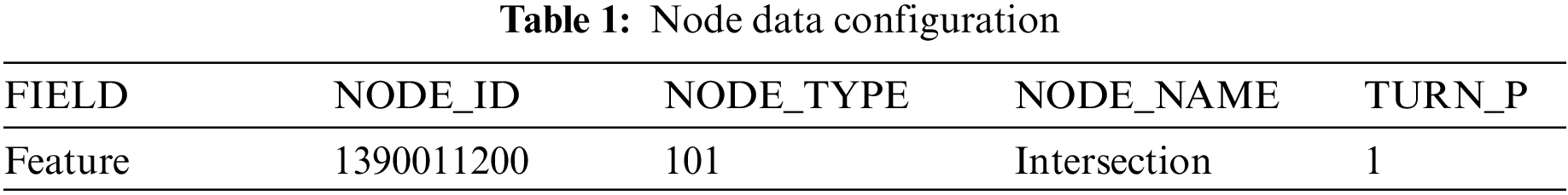
In Table 1, NODE_ID, NODE_TYPE, NODE_NAME and TURN_P indicate the unique number of the node, the type of the node, the name of the node, and whether rotation is restricted. In addition, the link data is a line connecting a node that is a speed change point and a node, and represents an actual road. This includes roads, overpasses, bridges, underpasses, and tunnels. Table 2 shows the link data configuration.

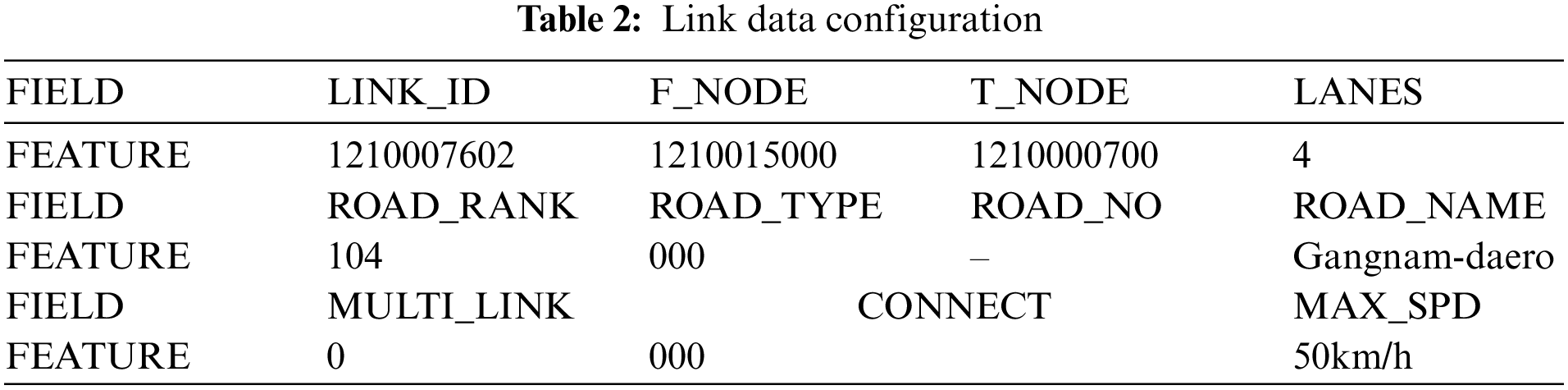
In Table 2, LINK_ID is the unique number of the link, F_NODE is the ID of the starting node, T_NODE is the ID of the ending node, LANES is the number of lanes, ROAD_RANK is the rank of the road, ROAD_TYPE is the type of the road, ROAD_NAME is the name of the road, MULTI_LINK indicates whether there is an intermediate section, CONNECT indicates the code of the link road, and MAX_SPD indicates the maximum speed limit of the road. Traffic speed data is collected through devices or equipment installed on the road. It is collected based on Location, Days, and Interval, and data missing exists according to the criteria. Fig. 5 shows the multidimensional matrix for the missing types and criteria for which traffic speed data are collected.

Figure 5: Multidimensional matrix for types with missing

In Fig. 5, speed data is collected based on three criteria. It is collected based on Day, Location, and Intervals. Missing exists in three types: Interval missing if traffic data should be collected every 5 min, but the entire data is not collected for that 5 min, Location missing if there are parts that cannot be collected by road, and Days missing if the entire day is not collected. In addition, if the size of the data feature is significantly different for each variable, the performance of the model becomes a problem, so data normalization is performed. There are two types of regularization methods: Min-Max regularization and Z-score regularization [21,22].

Min-Max regularization finds the minimum and maximum values for all features and sets them to 0 and 1, respectively. Values that exist between the minimum and maximum values are converted to values between 0 and 1. This has the disadvantage of being vulnerable to outliers, al-though all features have the same scale. Since velocity data contains a large amount of outliers, outliers are removed through the median absolute deviation and Min-Max normalization is performed. Eq. (2) shows the Min-Max regularization equation.

Min−Max=x−MinMax−Min(2)

In Eq. (2), x represents data, Min represents the minimum value of data, and max the maximum value of data. The denominator specifies the range of data by subtracting the largest and smallest values in the data. It also subtracts each data x and the minimum value from the numerator to determine where to place the data in the specified range. The Z-Score regularization method is a regularization method that can avoid the outlier problem. However, since each data value is not accurately normalized to the same scale, Min-Max normalization is performed on the values from which outliers are removed in this study.

3.2 Extraction of Spatiotemporal Features Using Spatial Temporal Layer

Traffic data has time series and spatial features. Therefore, the temporal convolution layer is used to capture and learn temporal features, and the spatio convolution layer is used to learn spatial features. In general, LSTM and GRU of RNN series are used to learn temporal features [23,24]. The disadvantage of LSTM, which is typically used, is slow learning time. Due to the nature of LSTM, the output of the model depends on previous data, so parallelization cannot be performed.

Thus, the amount of calculation increases according to the number of data during the calculation process, which slows down the calculation. Therefore, this study has an advantage in learning speed by enabling parallelization by using casual convolution and GLU activation function [25,26]. Fig. 6 shows the structure of the temporal convolution layer. In Fig. 6, casual convolution is a convolution operation used for data with temporal features. This makes the output value dependent only on the current input and past data at every step when performing the convolution operation. Also, to pass the GLU activation function, the dimension is doubled. By dividing the amplified tensor in half, sigmoid operation is performed for one part, while the Hadamard product for each element for the other part. It is the result of GLU operation and alleviates the vanishing gradient problem through linear operation while maintaining the non-linear function. In addition, GLU is more stable than Rectified Linear Unit (ReLU) and can learn faster than sigmoid. Eq. (3) shows the equation of GLU.

Figure 6: Structure of temporal convolution layer

v([AB])=A⊗σ(B)(3)

In Eq. (3), v means linear mapping, and σ means sigmoid activation. A and B represent the input values divided by half, and linear mapping is performed on them. A sigmoid operation is performed on the divided side. In addition, it means element-wise Hadamard product, and an element-wise Hadamard product is performed on a part different from the value of the sigmoid operation. During the GLU operation, the previous value is added to the remaining part that does not pass the sigmoid through the residual connection. This solves the tendency of network performance degradation as the number of network layers increases, that is, the learning set loss gradually decreases as the number of network layers increases and then becomes saturated. Temporal convolution layer is easier to learn than RNN and other models, has a simpler structure, and can be used for time series data. In addition, parallelization is possible and if layers of the CNN structure are stacked, the number of nonlinearities is reduced, solving the vanishing gradient problem compared to RNN. Next, the spatio convolution layer is used to learn spatial features. In general, data in graph form does not exist in Euclidean space. Therefore, it is difficult to apply learning using CNN. Therefore, a GCN that receives graph-type data as an input is used. In general, the adjacency matrix used in GCN expresses only the connection with the neighbor node, so its own information in the convolution operation is not considered when the latent feature vector is created. In this study, therefore, when implementing GCN, a self-loop is added to the adjacency matrix. Eq. (4) shows the operation expression of the graph convolution layer.

H(l+1)=σ(D−12~AD−12~H(l)W(l))(4)

In Eq. (4), Hl is the hidden state of the l-th layer, and H0 = X (initial feature of the graph node). Is, the addition of a self-loop to the adjacency matrix. Also, since the adjacency matrix is not normalized, the size of the feature vector may be unstable when multiplying the feature vector and adjacency matrix. Therefore, normalization is necessary. This creates a degree matrix according to the number of edges connected to each node and normalizes the adjacency matrix (A) to. In this case, is the degree matrix of the adjacency matrix. W(l) is a parameter of the l-th layer, and σ is a nonlinear function that uses the ReLU function.

3.3 Traffic Communication Data Missing Imputation Model Using Adversarial Auto Encoders

The structure of the Adversarial Auto Encoder (AAE) model, which combines the Variational Auto Encoder (VAE) and the GAN model, is used to impute missing of time series data. General GAN has the disadvantage that it is more difficult to learn the generator than the discriminator. Therefore, in this study, the AAE structure is used to promote the stability of learning. Fig. 7 shows the network configuration of the adversarial auto encoder-based missing imputation model.

Figure 7: Network configuration for the adversarial auto encoder-based missing imputation models

In the Fig. 7, the model consists of four modules: an encoder, a decoder, and two discriminators. Temporal convolution layer and spatio convolution layer are added to the encoder performing feature extraction to learn spatiotemporal features of data. In order to extract each feature, calculation is performed through a block that combines features by stacking layers. In order to input data to the model, it is necessary to fill the missing present in the data. To fill the missing, a real number between 0 and 0.01 is generated from the sample data and the sample is filled in the missing position through a mask matrix that defines the location of the missing. Fig. 8 shows the data input configuration of the model for missing imputation.

Figure 8: Configure the data input of the model for missing imputation

In Fig. 8, in order to compose the input value, the missing data (x), the mask (m) that displays the missing part, and the sample data (z) for learning by filling in the missing part are prepared. The existing data and the sample data (z) are combined through a mask. A mask is a matrix composed of 0 and 1. 0 means the missing part and 1 is defined as the presence of existing data. The mask data is multiplied by x, and the missing position is positioned as the sample data through the (1 − m) operation. The generated input data is input to the model. For the input data, learning is carried out through the model. The input data is subjected to feature extraction through the encoder. For the encoder part of the generator model, the feature extraction is performed through the temporal convolution layer and the spatio convolution layer. A latent distribution is created through the extracted data. The created latent distribution is input to the decoder to restore and generate data. Fig. 9 shows loss calculation process of generator model.

Figure 9: Loss calculation process of generator model

In the Fig. 9, the data generated through the generator model and the existing data are combined. Through the mask data, the existing data is left and only the generated data is put in the missing position. In addition, the generated data for the generator’s loss calculation is input to the discriminator model 1. For loss of the generator model, Mean Squared Error (MSE) loss operation is performed on generated by the generator and the existing data. Also, by inputting to discriminator model 1, cross entropy loss operation is performed with the mask data. Loss calculation of the generator model is performed through MSE operation and cross entropy operation. In the discriminator 1 model, cross entropy loss calculates the loss of the generated value and induces the generated value to be generated better, and induces existing values that have been subjected to MSE operation to be learned in a form similar to the existing form [26–28]. Fig. 10 shows the loss calculation process of the discriminator model through the latent vector.

Figure 10: Loss calculation process of discriminator model through latent vector

In the Fig. 10, the latent distribution and target distribution generated through the encoder are input to discriminator model 2 to perform the cross-entropy loss operation. The difference between discriminator models is that discriminator model 1 is directly involved in the loss of the generator model to help with data generation. In discriminator model 2, however, the discriminator model learns the difference between the actual value and the generated value to create an adversarial relationship, helping with learning of the generator model.

4  Experiment and Performance Evaluation

In this study, a system of Ubuntu 16.04, Intel Xeon Gold 5120 2.2 Ghz, 20TFlOPS GPU (NVIDIA Tesla V100 2 Way) is used as the experimental environment for performing the missing value correction experiment. In addition, traffic speed data are collected to carry out the experiment. As Traffic speed data, domestic ITS data and data provided by the California Highway System (PeMSD7) in the United States are collected from two sources. This is because domestic ITS data has a high missing rate, so it is not possible to conduct an experiment according to the missing rate. Therefore, through PeMSD7, an experiment according to the missing rate is conducted to evaluate the performance, and the effectiveness of the domestic data is proved [29,30]. For the spatial range of domestic data, 144 links in the Gangnam area are collected, while for the temporal range, weekday data from 2020/11 to 2020/12 are collected. Each data is the data for each link with a 5-minute period equally collected for 24 h a day. For the PeMSD7 data, data from 288 detectors in District 7 of California as a spatial extent are collected, and the temporal range is the same. Performance evaluation is carried out in three ways: Accuracy evaluation is carried out through performance comparison evaluation with existing data imputation method according to the missing rate, data imputation result graph according to the missing imputation method, and traffic congestion measurement according to the missing imputation algorithm. As evaluation indicators used for performance evaluation, Root Mean Squared Error (RMSE) and Mean Absolute Percentage Error (MAPE) are used for performance evaluation, respectively [31,32,33].

4.1 Performance Comparison Evaluation with Existing Data Imputation Methods According to the Missing Rate

The performance with that existing models is compared according to the missing rate. To evaluate the performance of the model according to the missing rate, 10–50% of the missing rate of the data is randomly removed to generate the missing in the data set. As data, California highway system data is used, and the evaluation index is RMSE. The lower, the better the performance. Table 3 shows the performance comparison results with existing models according to the missing rate [7,8,11,12].

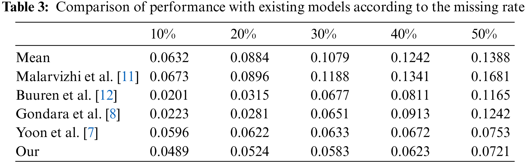
In Table 3, each of the existing research models shows better performance between missing rates of 10% to 20%, but the proposed model has the better performance between 30% and 50%. In addition, the existing studies, which showed good performance at missing rates of 10% to 20%, show that the results diverge greatly from the results of 30%, but the results of the proposed model show stable performance from start to finish. It is analyzed that the data was imputed relatively well compared to the existing studies despite the large number of missing rates because it fills the missing by creating it through the data distribution, which is the feature of the model.

4.2 Data Imputation Result Graph According to Missing Imputation

The second performance evaluation confirms the pattern of each result value by expressing the data completed through the missing imputation model as a graph. It is compared with the adversarial generative neural network-based GAIN model, which has shown stable performance [9]. A qualitative comparison is carried out through graphs by imputing data with missing values with complete data through the model. The data used consists of US data with a missing rate of 30%. Fig. 11 shows a graph comparing actual data and missing data. In Fig. 11, the red line indicates the missing part and the actual value, and the green indicates the non-missing part. Fig. 12 shows the data imputation result graph according to the imputation method.

Figure 11: Comparison graph of real data and missing data

Figure 12: Data imputation result graph according to missing imputation method

In the graph, the X-axis represents time and means the interval of 5 seconds per point, while the y-axis represents speed. In the graph in Fig. 12, the blue dotted line is the result value of GAIN, and the black solid line is the result value of the proposed study. In Fig. 12, the red line, where the missing part exists, is compared with the result graph of the imputation model to check whether the data of the missing point is well generated. The graph shows that the graph of the proposed model as a whole generates a relatively good pattern at the missing point. It is analyzed that the spatiotemporal feature extraction layer added to the encoder part of the model correctly learned the features of the data. However, the graph shows in detail that the pattern of the actual data is generated relatively similar to that of GAIN, but there is a part where the value bounces.

4.3 Accuracy Evaluation Through Traffic Congestion Measurement According to Missing Imputation

As a final performance evaluation, time series performance is identified using data with missing imputed through the models of existing studies [33]. Time series prediction is performed after complete data generation through missing imputation models. The data used at this time consists of domestic ITS data (data missing 30%). In addition, the post-missing traffic congestion measurement model uses the RNN family of LSTMs, which are used for time series prediction. The output value configuration is designed to predict road speed after 5 minutes from the current time of the link. The performance evaluation index is MAPE, and the lower, the better the performance. Fig. 13 shows the comparison results of time series prediction performance according to the missing imputation method.

Figure 13: Comparison of time series prediction performance according to missing imputation method

In Fig. 13, the model replacing the missing value through the average shows the lowest performance. Next, Malarvizhi et al. [11] with k-NN shows a performance of 12.42, and Gondara et al. [8] with Imputation using a denoising autoencoder shows results of 8.56. Next, Buuren et al. [12], which substitutes missing values through Multivariate Imposition by Chained Equations, shows a performance of 8.23. Yoon et al. [7], who substituted missing values using adversarial artificial neural networks, is 6.45, showing the best performance among existing studies. However, the proposed model's performance is considered the best compared to existing studies. Thus, the data pattern is well generated, which can be analyzed to demonstrate the effectiveness of time-to-time feature extraction.

5  Conclusions

In this study, we proposed the imputation of missing values by reflecting the temporal and spatial characteristics of traffic data using temporal convolution and spatial convolution. The experiments showed that outliers and missing values in traffic data affect the results when making predictions. In order to improve the performance of the model when predicting congestion and speed through traffic data, missing values were imputed and outliers were removed from the collected data. The AAE model was used as the basis for the data imputation model. This is a model that complements the shortcomings of GAN and AE. In addition, temporal characteristics of traffic data are important, but spatial characteristics are important as well. Therefore, graph convolution was used to learn spatial features, and temporal features were constructed using causal convolution and gated linear unit activation functions. In order to verify the performance of the model, the performance evaluation is performed through three methods. It consists of performance comparison with the existing data imputation method according to the missing rate, data imputation graph results according to the missing imputation method, and time series prediction performance comparison according to the missing imputation method. In the first performance evaluation, each existing research model showed better performance with missing rates of 10% to 20%, but in the case of the performance between 30% and 50%, the proposed model showed relatively good results. The second performance evaluation identifies the pattern of each result value by expressing the data completed through the missing imputation model as a graph. It was found that the graph of the proposed model shows a good shape at the relatively missing point. Finally, in the third performance evaluation, the time series performance is verified using the data with missing imputed through the models of existing studies. The model imputed through the average shows the worst performance of 15.64%, the GAN-based model shows a relatively good performance of 6.45%, and the performance of the proposed model is relatively good, 5.92%, leading to the analysis that the pattern of the data has been well generated. Through this study, the problem of data sparseness was solved and the performance of the predictive model was improved. As a future study, we plan to conduct a model study so that missing imputation can be performed well even with a large number of missing rates, and a traffic congestion prediction model study through the imputed data.

Funding Statement: This research was supported by the MSIT (Ministry of Science and ICT), Korea, under the ITRC (Information Technology Research Center) support program (IITP-2018-0-01405) supervised by the IITP (Institute for Information & Communications Technology Planning & Evaluation).

Conflicts of Interest: The authors declare that they have no conflicts of interest to report regarding the present study.

References

1. S. E. Ryu, D. H. Shin and K. Chung, “Prediction model of dementia risk based on XGBoost using derived variable extraction and hyper parameter optimization,” IEEE Access, vol. 8, pp. 177708–177720, 2020. [Google Scholar]

2. D. H. Shin, R. C. Park and K. Chung, “Decision boundary-based anomaly detection model using improved AnoGAN from ECG data,” IEEE Access, vol. 8, pp. 108664–108674, 2020. [Google Scholar]

3. H. J. Kwon, M. J. Kim, J. W. Baek and K. Chung, “Voice frequency synthesis using VAW-GAN based amplitude scaling for emotion transformation,” KSII Transactions on Internet and Information Systems, vol. 16, no. 2, pp. 713–725, 2022. [Google Scholar]

4. C. M. Musil, C. B. Warner, P. K. Yobas and S. L. Jones, “A comparison of imputation techniques for handling missing data,” Western Journal of Nursing Research, vol. 24, no. 7, pp. 815–829, 2002. [Google Scholar] [PubMed]

5. P. A. Patrician, “Multiple imputation for missing data,” Research in Nursing & Health, vol. 25, no. 1, pp. 76–84, 2002. [Google Scholar]

6. I. Spinelli, S. Scardapane and A. Uncini, “Missing data imputation with adversarially-trained graph convolutional networks,” Neural Networks, vol. 129, no. 1, pp. 249–260, 2020. [Google Scholar] [PubMed]

7. J. Yoon, J. Jordon and M. Schaar, “Gain: Missing data imputation using generative adversarial nets,” in Int. Conf. on Machine Learning, Stockholm, Sweden, pp. 5689–5698, 2018. [Google Scholar]

8. L. Gondara and K. Wang, “Mida: Multiple imputation using denoising autoencoders,” in Pacific-Asia Conf. on Knowledge Discovery and Data Mining, Cham, Springer, pp. 260–272, 2018. [Google Scholar]

9. P. Wu, L. Xu and Z. Huang, “Imputation methods used in missing traffic data: A literature review,” in Int. Symp. on Intelligence Computation and Applications, Singapore, Springer, pp. 662–677, 2020. [Google Scholar]

10. A. B. Pedersen, E. M. Mikkelsen, D. C. Fenton, N. R. Kristensen, T. M. Pham et al., “Missing data and multiple imputation in clinical epidemiological research,” Clinical Epidemiology, vol. 9, pp. 157, 2017. [Google Scholar] [PubMed]

11. R. Malarvizhi and A. S. Thanamani, “K-nearest neighbor in missing data imputation,” International Journal of Engineering Research and Development, vol. 5, no. 1, pp. 5–7, 2012. [Google Scholar]

12. S. Van Buuren and K. Groothuis-Oudshoorn, “MICE: Multivariate imputation by chained equations in R,” Journal of Statistical Software, vol. 45, no. 3, pp. 1–67, 2011. [Google Scholar]

13. T. H. Lin, “A comparison of multiple imputation with EM algorithm and MCMC method for quality of life missing data,” Quality & Quantity, vol. 44, no. 2, pp. 277–287, 2010. [Google Scholar]

14. D. J. Stekhoven and P. Bühlmann, “MissForest-non-parametric missing value imputation for mixed-type data,” Bioinformatics, vol. 28, no. 1, pp. 112–118, 2012. [Google Scholar] [PubMed]

15. A. G. Schwing and R. Urtasun, “Fully connected deep structured networks,” arXiv preprint arXiv: 1503.02351, 2015. [Google Scholar]

16. M. Lin, Q. Chen and S. Yan, “Network in network,” arXiv preprint arXiv: 1312.4400, 2013. [Google Scholar]

17. Y. LeCun and Y. Bengio, “Convolutional networks for images, speech, and time series,” The Handbook of Brain Theory and Neural Networks, vol. 3361, no. 10, pp. 1995, 1995. [Google Scholar]

18. T. N. Kipf and M. Welling, “Semi-supervised classification with graph convolutional networks,” arXiv preprint arXiv: 1609.02907, 2016. [Google Scholar]

19. Z. Cui, K. Henrickson, R. Ke, Z. Pu and Y. Wang, “Traffic graph convolutional recurrent neural network: A deep learning framework for network-scale traffic learning and forecasting,” arXiv preprint arXiv: 1802.07007v3, 2018. [Google Scholar]

20. S. Patro and K. K. Sahu, “Normalization: A preprocessing stage,” arXiv preprint arXiv: 1503.06462, 2015. [Google Scholar]

21. S. Bhanja and A. Das, “Impact of data normalization on deep neural network for time series forecasting,” arXiv preprint arXiv: 1812.05519, 2018. [Google Scholar]

22. D. H. Shin, “Spatiotemporal feature extraction based missing value imputation model for predicting time series data,” M.S. Thesis, Department of Computer Science, Kyonggi University, Suwon-Si, South Korea, 2021. [Google Scholar]

23. K. Cho, B. Van Merriënboer, C. Gulcehre, D. Bahdanau, F. Bougares et al., “Learning phrase representations using RNN encoder-decoder for statistical machine translation,” arXiv preprint arXiv: 1406.1078, 2014. [Google Scholar]

24. T. J. Brazil, “Causal-convolution—A new method for the transient analysis of linear systems at microwave frequencies,” IEEE Transactions on Microwave Theory and Techniques, vol. 43, no. 2, pp. 315–323, 1995. [Google Scholar]

25. J. Veness, T. Lattimore, D. Budden, A. Bhoopchand, C. Mattern et al., “Gated linear networks,” in Proc. of the AAAI Conf. on Artificial Intelligence, Palo Alto, California, USA, pp. 10015–10023, 2021. [Google Scholar]

26. H. K. Khang and S. B. Kim, “Missing data imputation with adversarial autoencoders,” in Proc. of the Korean Institute of Industrial Engineers Fall Conf., Seoul, Korea, pp. 1867–1895, 2019. [Google Scholar]

27. H. Marmolin, “Subjective MSE measures,” IEEE Transactions on Systems, Man, and Cybernetics, vol. 16, no. 3, pp. 486–489, 1986. [Google Scholar]

28. U. Sara, M. Akter and M. S. Uddin, “Image quality assessment through FSIM, SSIM, MSE and PSNR—A comparative study,” Journal of Computer and Communications, vol. 7, no. 3, pp. 8–18, 2019. [Google Scholar]

29. California Department of Transportation, 2020. [Online]. Available: https://pems.dot.ca.gov/ [Google Scholar]

30. Q. Shao, Y. Zhang, D. Chen and W. Yu, “GLGAT: Global-local graph attention network for traffic forecasting,” in 2020 7th Int. Conf. on Information, Cybernetics, and Computational Social Systems (ICCSS), Guangzhou, China, pp. 705–709, 2020. [Google Scholar]

31. C. O. Plumpton, T. Morris, D. A. Hughes and I. R. White, “Multiple imputation of multiple multi-item scales when a full imputation model is infeasible,” BMC Research Notes, vol. 9, no. 1, pp. 1–15, 2016. [Google Scholar]

32. S. Kaffash, A. T. Nguyen and J. Zhu, “Big data algorithms and applications in intelligent transportation system: A review and bibliometric analysis,” International Journal of Production Economics, vol. 231, no. 3, pp. 107868, 2021. [Google Scholar]

33. B. U. Jeon and K. Chung, “CutPaste-based anomaly detection model using multi-scale feature extraction in time series streaming data,” KSII Transactions on Internet and Information Systems (TIIS), vol. 16, no. 8, pp. 2787–2800, 2022. [Google Scholar]