A Sensor Network Coverage Planning Based on Adjusted Single Candidate Optimizer

1  Introduction

Wireless sensor networks (WSNs) are made up of a number of low-power sensor nodes with communication capabilities [1] that are widely used in a variety of fields, including environmental monitoring, urban management, agricultural control, and military applications [2,3]. The ways of the WSN differ from a traditional wireless network, such as [4]. It features more nodes than a conventional wireless network, but energy conservation is important because each node is made to be powered mostly by batteries [5,6]. The placement of the nodes is frequently highly uncertain—for some design reasons, it could even be classified as harsh—which could cause some errors in the location signal [7]. It is often utilized across the Internet or cloud environment [8,9] because it has the beneficial properties of WSN, such as self-organization, speed, practicality, and ease of deployment [10]. In order to monitor environmental and physical conditions, the WSN network [11] is equipped with the minute parts of heterogeneous or homogeneous sensor nodes [12]. As its name implies, the sensor node may perceive, act upon, and wirelessly communicate the data gathered from the source environment to the sink or base station [13]. One of the most fundamental issues with WSNs is the node coverage in a whole network, and coverage is a crucial indicator for assessing service optimization techniques [14]. Because it directly affects WSN applications [15], e.g., the target monitoring area’s monitoring capacity, and coverage substantially impacts the WSN’s quality of service [16]. Rational and efficient sensor node deployment reduces network expenses and energy consumption [17]. WSN coverage applications aim to efficiently deploy several sensor nodes to monitor a target region of interest [10,18]. Target tracking, combat monitoring, etc., and require higher network coverage levels [19]. The vast majority of sensor nodes are dispersed randomly over the intended monitoring area, leading to limited coverage and an uneven distribution of sensor nodes [20]. As a result, it is crucial to strategically place sensor nodes to maximize the node coverage of WSNs in the monitoring zone [21]. Finding the best solution under these circumstances remains challenging because the rational and effective deployment of WSN is an NP-hard problem for large-scale sensor node deployment challenges [22].

A WSN’s coverage must ensure that the area is monitored with the necessary level of dependability. Further specifications for network coverage levels are needed for various application scenarios [21,23]. Other applications, including smart agriculture and environmental monitoring, require lower network coverage levels [24]. Large-scale sensor node deployment issues have shown that the efficient and logical deployment of WSNs is a challenging problem; determining the best answer in such circumstances is still tricky [25]. Moreover, as sensor networks are used widely [26,27], more and more applications call for the precise placement of sensor nodes [28]. Much effort is put into moving sensor nodes around using optimization methods to increase network coverage [29]. The algorithms that analyze the network’s coverage rely heavily on the positions of the sensor nodes; after that, the optimization algorithms are employed to enhance network coverage and minimize or eliminate network blind spots [30].

Over the last two decades, the research field of meta-heuristic intelligence algorithms [31] has been very active, and new meta-heuristic algorithms have been proposed constantly [32]. The meta-heuristic algorithm is a stochastic optimization algorithm suitable for real-world optimization problems [33,34]. Among them, genetic algorithms (GAs) [35], particle swarm optimization (PSO) [36], and gravitational local search (GLSA) [37], Single Candidate Optimizer (SCO) [38], etc., are well-known. The metaheuristic one used the meta-heuristic algorithm to optimize WSN’s network coverage and eliminate the coverage holes in the interest areas of the network effectively [39]. The metaheuristic algorithm constitutes one of the promising solutions for optimal WSN node coverage compared to the traditional methods [40]. With the limited computational resources of the WSN, metaheuristic algorithms can find close to ideal solutions in a reasonable executive time, making them a practical answer to the network coverage optimization problem [41].

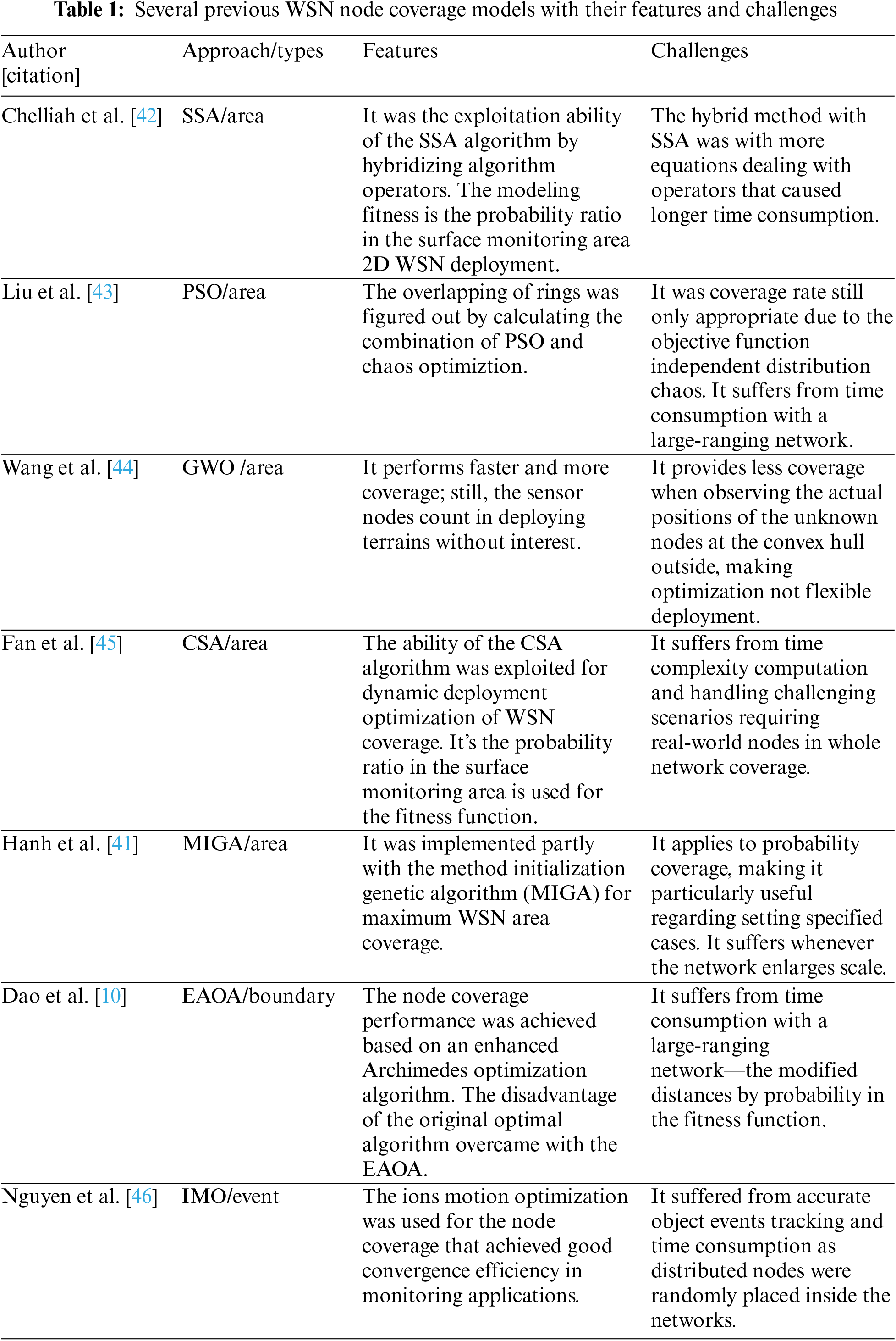
Table 1 lists the summarized review of previously selected related works with WSN node coverage models with their features and challenges. Three techniques, e.g., area, boundary, and event coverage categories, have challenges with low coverage rate and time computation complexity whenever the network is enlarged scale.

The SCO algorithm is a recent metaheuristic algorithm that is taken inspiration from a single-candidate solution for the optimization process [38]. A set of equations includes the location updating equations toward the target solution based on its fitness values of the candidate solution throughout the whole optimization process. An integrated switching variable strategy is for balance exploration and exploitation of target searching optimal solution for SCO updating candidate solution positions differently in each phase [38]. The SCO algorithm has several advantages, e.g., concept simplicity, robust process, and ease of implementation; still, it has limitations in the ratios of exploration and exploitation for avoiding the local optimum trap when dealing with a complicated problem like node coverage optimization situations.

This study proposes an optimal strategy for sensor node coverage in WSNs deployed in sensing regions, utilizing an adjusted single candidate optimizer (ASCO). The ASCO algorithm is implemented by incorporating stochastic reverse learning and multi-direction strategies to address the limitations of its original version and solve the network coverage. The aim is to achieve efficient and logical deployment of WSNs, which significantly impacts network performance [39].

The objective function of the WSN node coverage optimization problem is modeled by placing each deployed node with a fixed sensing radius, limiting their perception capabilities to specific areas [10,46]. The coverage rate, representing the ratio of the covered area by sensor nodes to the total monitoring area, is used as the fitness value. Each sensor’s sensing range is confined to its assigned deployment area, and the coverage ratio is calculated using the probability ratio in the 2D WSN monitoring network.

To demonstrate the potential performance of the ASCO algorithm, it is tested against the objective function of the node coverage problem and compared with other widely used algorithms in the literature. The experimental results highlight the efficiency of the designed coverage scheme, considering various metrics such as coverage rate, positioning errors, coverage speed, and execution time. The comparative analysis demonstrates that the ASCO scheme offers a highly applicable coverage model, enabling excellent quality in network deployment applications. The suggested approach makes significant contributions in the following areas:

•   Strategies are proposed to adapt the ASCO algorithm, mitigating the limitations of its original version and enhancing its performance in complex node coverage optimization scenarios.

•   The suggested ASCO approach establishes an effective solution for addressing the issue of optimal WSN node coverage.

•   The performance of the suggested method is evaluated through rigorous testing, including comparison with other algorithms in the literature. The experimental results are analyzed and discussed, providing valuable insights into the effectiveness of the ASCO algorithm.

The remaining sections of the paper are structured as follows. The literature on conventional node coverage strategies in WSN and the node coverage model paradigm is reviewed in Section 2. Section 3 presents a novel ASCO based on SCO with a stochastic reverse learning strategy and multi-direction control factor. Section 4 illustrates the ideal node coverage strategy and the simulation outcomes analyzed. Section 5 concludes with a comprehensive analysis of the inventive scheme.

2  Related Work

2.1 WSN Coverage and Connection Model

A statement of maximum coverage planning in the WSN node coverage efficiency is modeled for the optimization issue [21]. For the optimization model problem, the WSN node coverage definition is known as each deployed node in WSN with a fixed sensing radius that a desired placement sensor can only sense in arrange to reach each other [10]. At the beginning of experiments, sensor nodes are randomly placed only to feel and discover that a WSN isomorphic within its sensing radius in monitoring the interest area. The metaheuristic method is then used to position-optimize the wireless sensor nodes to maximize WSN coverage [25]. As a result, each node needs to be placed within a limited sensing range to communicate with the rest of the network and each other. The coverage problem of finding objects inside of it in potential optimization ranges is well met by its sensing radius.

A two-dimensional monitoring region is divided into W⋅L grids that looked at as a monitoring point p at the center of a grid. The two-dimensional coordinators of every point p are indicated as (x, y), where the x and y are integers, and the value of x and y range from 1 to L and from 1 to W, respectively. The coordinator x denotes the row index of the grid, while y refers to the column index. The two dimensional coordinators of the grid, which are in row i and column j within the monitoring area, are represented as (i,j).

A set of sensor nodes is assumed isomorphic and randomly deployed in the monitoring area, which is indicated as =[n1,n2,…,ni,…,ns], while s is the number of sensor nodes. The two-dimensional coordinators of any sensor node ni in the set are denoted as (xi,yi). The positions of the sensor nodes in the monitoring area are indicated as P=[(x1,y1),(x2,y2),…,(xi,yi),…,(xs,ys)]. The radius of sensor nodes is represented as Rs.Two models calculate the sensing range of the sensor nodes. One is the binary model, and the other is the probabilistic model. In the binary model, the sensing range of a sensor node is calculated by the Euclidean distance given as follows:

di=(xi−x)2+(yi−y)2,(1)

where (xi,yi) is the coordinator of the sensor node ni; (x, y) denotes the coordinator of monitoring point p, and di is the distance between ni and p. The binary model, which presupposes there are no interferences and no attenuation of wireless signals in the WSN environment, does not take into account the complexity of the WSN network environment. While the wireless signal intensity will gradually decrease with an increase in transmission distance, there are wireless signal interferences between nodes and from other noise sources in the natural wireless transmission environment. As indicated above, the complexity of the wireless signal transmission environment is considered by the probabilistic perception model used in this research.

In the probabilistic perception model, the probability that the sensor node ni covers the monitoring point p is denoted as follows:

Pc(x,y,ni)={1,if d(ni,p)≤Rs−ree(−α1λ2β2)λ2β2+α2if Rs−re<d(ni,p)<Rs+re0,if d(ni,p)≥Rs+re,(2)

where re indicates the reliability parameter of the sensor node, and 0 < re < Rs; α1, α2, β1, and β2 are measurement parameters related to the characteristics of the sensor node; λ1 and λ2 are defined as follows:

{λ1=re−Rs+d(ni,p)λ2=re−Rs+d(ni,p),(3)

Suppose that a monitoring point p is covered by multiple sensor nodes, defined as Cr, Cr∈Cs. The probability calculation formula describing this event is indicated as follows:

Pc(Cr)j=1−∏ni∈Cr(1−Pc(x,y,ni)),(4)

where 1≤j≤(W⋅L). Calculate the coverage probability of every monitoring point, then the coverage rate of the monitoring area is calculated as follows:

R=∑j=1MPc(Cr)jW⋅L,(5)

where W⋅L is the network deployed area in 2D; R presented as the coverage ratio of WSN nodes, Pc(Cr)j indicates as the probability of the target point reaching sensed node monitoring.

The model of a two-dimensional WSN monitoring region network is assumed as follows. The re and Rs: the communication radius and sensing radius of each sensor node are both in meters units with re≥2Rs. The sensor node typically has the ability to communicate, is sufficiently powered, and has access to data. The specifications, structure, and communication capacities of the sensor node are all in the same condition. The mobile sensor node can quickly update its location by calculating the coverage ratio with the ratio of the probability of the network deployed surface 2D WSN monitoring area.

2.2 Single Candidate Optimizer

A recent metaheuristic algorithm is taken inspiration from a single-candidate solution (SCO) for the optimization process [38]. The updating position equations are described mathematically toward the target solution based on the fitness values of the candidate solution that is carried out via its set of expressions throughout the optimization process. The SCO has some stages of candidate solutions for the optimization process, e.g., initialization, exploiting, and exploring phases. The equations of updating solutions are the operation phases based on the candidate solution’s fitness values throughout the optimization process.

The first stage of SCO: the initialization phase: a candidate solution is generated randomly as follows.

Si=rand×(UBi−LBi)+LBi,(6)

where Si is the position of the i-th solution in the j-dimensional space as the matrix solution of the optimization method; N and n are the number of agents and the dimension of the search problem space. The initialization solution is generated randomly. Among them: UBi and LBi are the upper and the lower of the problem boundaries, respectively; rand is a random number between ∈ [0, 1]. Let Sbesti be the best candidate solution in each iteration is considered as the best-obtained solution or nearly the optimum so far based on the objective function.

The second stage of SCO: the exploitation stage, is the candidate solution of the SCO updated its locations as follows.

Si={Sbesti+(ω|Sbesti|),if r1≤0.5Sbesti−(ω|Sbesti|),otherwise,(7)

where r1 and ω are a variable of random number with ∈ [0, 1] and a variable of weight, respectively. The stage is conducted a deep search and searching continuously by thoroughly investigating the area surrounding the best location found in the previous generation or iteration. The optimization space that needs to be explored gradually gets close target as global optimization as the exploring phase progresses, making it easier to concentrate exclusively on potential areas.

The third stage of SCO is the exploring phase, which could be separated into sub-updating equations: weighted and standard subphase. A strategy can enhance solution population diversity by switching between weighted and standard subphases. A supporting binary variable is used to determine which one selected direction toward adding weight or not for enhanced agent’s diversity population. The candidate solution updates its positions in the following equation with the weighted subphase.

Si={Sbesti+(r2ω(UBi−LBi)),if r2≤0.5Sbesti−(r2ω(UBi−LBi)),otherwise,(8)

where r2 is a variable of random number ∈ [0, 1], UBi and LBi are the upper and lower boundaries of the limited problem space, respectively; In the standard sub-phase of SCO, a candidating solution is given for updating the position as follows:

Si={Sbesti+(r3(UBi−LBi)),if r3≤0.5Sbesti−(r3(UBi−LBi)),otherwise,(9)

where r3 is a variable of a random number with value ϵ [0, 1]. The candidate solution can switch from exploitation to exploration over updating position, which helps it escape the local optimum.

Additionally, changing the positions of some variables occasionally results in their values straying from their expected range or limits. The updated positions are set as follows in cases where variables’ values are greater than their upper bounds and lower bounds, respectively, to prevent them from exceeding the boundaries.

Si={Sbesti,if Si≤UBiSbesti,ifSi≤LBi,(10)

A candidate solution is assigned the same value as the global best value if the updated position goes out of bounds. The steps of the proposed algorithm are presented as a pseudocode as follows. The algorithm process often begins with randomly generating a matrix of the candidate solution in the search space. The objective function is evaluated over the candidate solution as its fitness, recording the candidate’s global best position Sbesti and its fitness f(Sbesti) for the best global fitness. A pseudocode of the SCO algorithm is shown in Algorithm 1.

3  Sensor Network Coverage Planning Using ASCO

This section presents the strategy for the adapted single candidate optimizer (ASCO) algorithm for optimal node coverage planning in WSN. The stochastic reverse learning initialization and modifying the exploiting phase in the search direction are used to adapt the algorithm of the ASCO for enhancing optimal coverage planning. Context subsections are presented as follows: adapted single candidate optimizer and modeled node coverage planning as an objective function for using the optimization strategy of the ASCO algorithm.

3.1 Adapted Single Candidate Optimizer

In this subsection, we present an adapted strategy based on the SCO with a suggested stochastic reverse learning method for initialization, direction agent moving, and inertia modification weight to enhance the performance optimal application algorithm. In the metaheuristic algorithm, the initial population phase is one of the influential factors in the processing search for optimum performance, special for the NP-complicated problem like the WSN coverage. A candidate solution is set as a matrix that is generated randomly as the initialization phase. A high-quality individual is selected with the same number as the initial population to form new agents by generating reverse solutions can effectively enhance the diversity of solutions and be closer to the optimal solution.

S=|s1,1s2,1..s1,Ds2,1s2,2..s2,D........sN,1sN,2..sN,D|,(11)

Here, S is the position of the i-th solution in the j-dimensional space as the matrix solution of the optimization method; N and D represent the number of agents and the dimension of the search problem space. The generated agent’s population by the reverse solution will achieve a new population as the elite population that will be integrated into the single solution optimizing process. The opposition learning is defined as follows:

Sm′=r4⋅(u+e)−Sm,(12)

Here, u and e represent the search space of the problem’s upper and lower bounds; Sm′ and Sm represent new and current individual solution positions that selected in [u, e]; r4 represent the random number ϵ [0, 1]. The initial population is also applied with a reverse mechanism that is a good effect on increasing population diversity and improving population quality. Then use the reverse and current solutions to select excellent individuals to generate a new population for initialization phase.

The metaheuristic algorithm may need to modify the balance based on the problem’s complexity. An adapted strategy is carried out in the ASCO that is reformulated as follows and because of capabilities exploiting phase Eq. (7) of the original algorithm has with just two search directions with a navigation coefficient τ may be equal + 1 or −1 in Eq. (7) that can be given as Si=Sbesti+τ⋅(ω|Sbesti|). The coefficient τ is expressed as follows:

τ={+1,if r1≤0.5−1,otherwise,(13)

The space for the complex problem may have more dimensions reaching into the target movement of the search space problem. By adding a random integer, it is possible to generate without repetition elements selected at random from the integers, resulting in many search directions. The alternate updating equation for exploiting direction is added with a new coefficient of guiding factor.

Si=Sbesti+τnew⋅(ω|Sbesti|),(14)

The formula expression of the τnew is a new guiding factor coefficient for motion direction is as follows:

τnew={+1⋅rand(),if r1≤0.5−1⋅rand(),otherwise,(15)

An integrated switching variable strategy is for balancing sub-explorations at the last stage of target searching optimal solution for updating candidate solution positions differently in each sub-phase. A binary switching variable p is used as marked candidate solution success for counting period switching.

p={1,if f(S)<f(Sbest)0,otherwise,c=c+1,(16)

Updated candidate solution positions in exploration phase are given for both sub-explorations at the last stage of target searching optimal solution as a new updating one.

Snew={S∈Eq.(8),if(c!=m)S∈Eq.(9),otherwise,c=0,(17)

Moreover, the weights need to be considered as an effect on the optimization performance of the algorithm. It means the weight parameter ω in SCO impacts the exploitation and exploration calculation as it decreases exponentially as function evaluations increase. Because the weight variable in the original algorithm uses the equation with the exponential calculation that causes complex process computation slowly, the weight needs to be adjusted with threshold-specific boundaries and calculated linearly. The weight is adjusted as follows:

ω(t)=(ω2−ω1)MaxIter−tt+ω1,(18)

where t and MaxIter T are variables of the current iteration and the max number of iterations, respectively; ω1 and ω2 are adjusting coefficient constants, which ω1 and ω2 are set 0.3 and 0.8, respectively. A relatively large value at the beginning of the search process helps effectively investigate the phase in the search area; therefore, the behavior is crucial as the weight parameter impacts the exploitation while iteration increases. On the other hand, when weight is a low value that enhances the exploiting phase in the last stages of optimization. The alternating weight is replaced with the weight in the original algorithm for the optimal network coverage planning problem. Algorithm 2 illustrates a pseudocode of the ASCO algorithm.

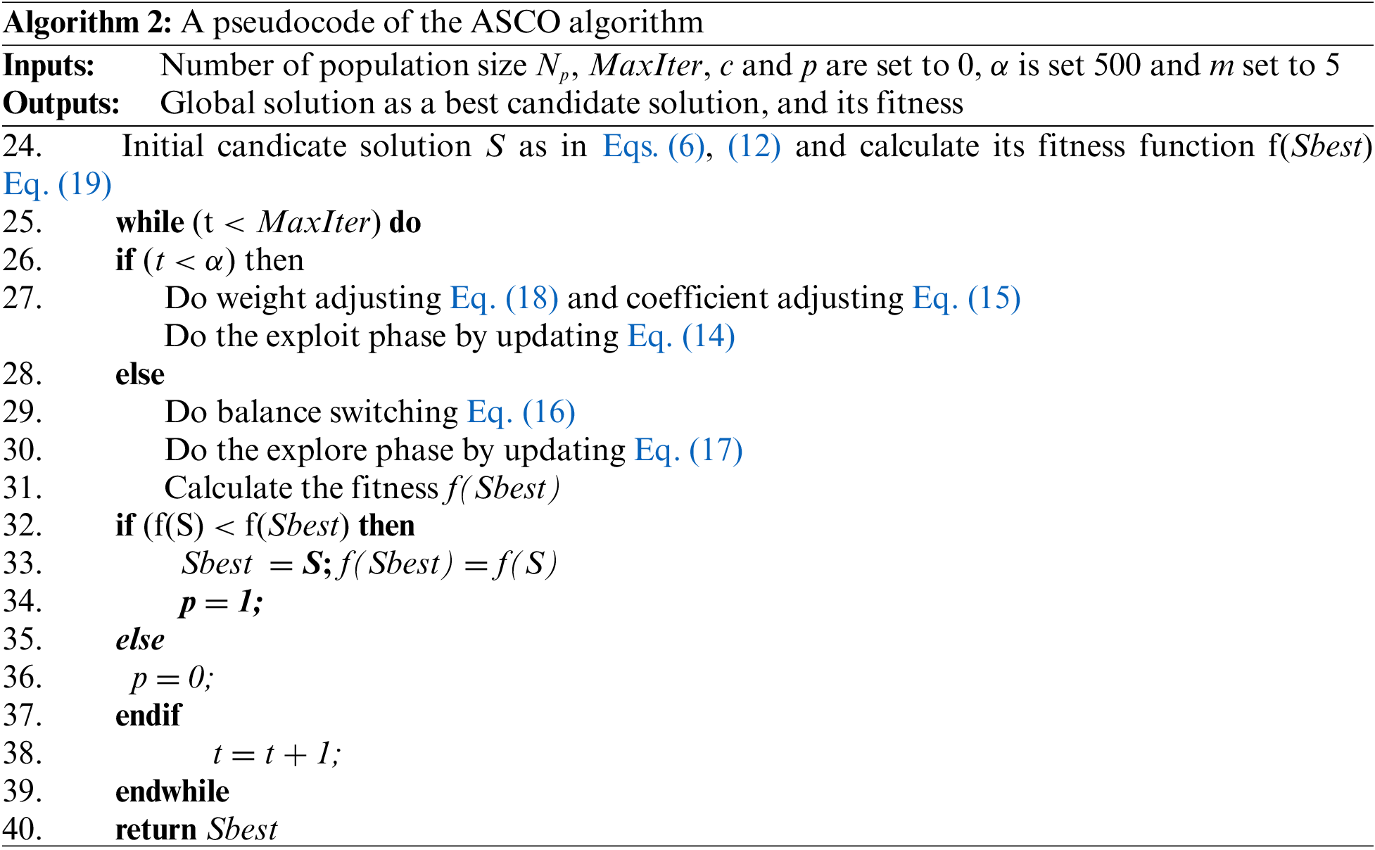
Fig. 1 illustrates a flow chart of applying the ASCO approach for optimal sensor network coverage planning related to the WSN deployment.

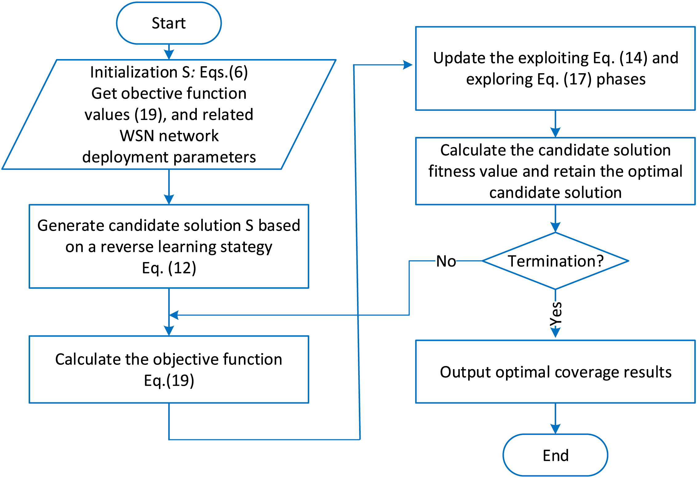
Figure 1: A flow chart of applying the ASCO approach for optimal sensor network coverage planning

3.2 Objective Function Coverage Strategy Using ASCO

This description presents how the ASCO algorithm implements the best node coverage for the WSN deployment. The majority of processing steps, analyses, and discussion outcomes are broken down into the following subsections. The most suitable solution to the optimal coverage planning challenge is the accurate placement of every deployed node in the WSN. The way by which different agents’ movement behaviors are organized toward the best answer or a particular area is the general formulation of the node’s location-seeking process. We apply the ASCO approach for WSN coverage optimization by seeking to maximize coverage of the target monitoring region by employing a small number of sensor nodes and arranging them strategically throughout the target monitoring area. Using the coverage ratio, we establish the optimal coverage planning model as the objective function. The best probability ratio is figured out to the surface monitoring area 2D WSN deployment, is the appropriate formula’s maximization seems to resemble follows:

Maximize Cov(R)=∑j=1MP(Cr)jW⋅L,(19)

where P(Cr)j is a variable of the probability of reaching target points in sensing node of the monitoring 2D as W⋅L (width and length) network deployed area; M is a number of nodes in sensor network; Maximize Cov(R) is the objective function as a fitness of WSN nodes optimal coverage model; Cov(R) a variable that represents the coverage ratio of nodes with planets locations as a coverage distribution. The following step list consists of the specific algorithm processes used in the optimal coverage planning strategy.

Step 1 Inputs involved in deploying the sensor network are set with parameters consisting of, e.g., W⋅L: area of a deployed region, M: the number of nodes, Rs: sensing radius, ω1 is set to 0.3 and ω2 is set to 0.8.

Step 2 Variables and parameters involving the algorithm are set, e.g., Np: number of population solution size is set to 2000, MaxIter: max number of iterations is set to 1000, c and p are set to 0, α is set 500 and m set to 5.

Step 3 Solution initializing population using reverse learning approach Eqs. (6) and (12) the objective function Eq. (19) with best fitness values for initial node coverage optima in the sorting range, set as in Table 1.

Step 4 Executing the optimal coverage planning process is figured out with updating equations of exploiting and exploring phases Eqs. (7) and (17) the for solution locations.

Step 5 Then compare with a new solution location to choose the highest fitness value based on the objective function Eq. (19). Compute the individual solution value and back up the optimal solution value of the global best of the node locations values.

Step 6 Check whether the terminating condition procedure is met; if so, move on to the next step; if not, go to step 4.

Step 7 The scheme terminates and generates the most desirable solution and the optimum fitness value, which indicates that the node’s optimal coverage rate is produced.

4  Analysis and Discussion Results

It is accessible for setting the experimental scenario for the sensor network deployed area to assume that the sensor nodes of the WSN are placed in a deployment monitoring W×L areas, e.g.,80 × 80 m2, 100 × 100 m2, 160 × 160 m2 and 300 × 300 m2. The specifications for experimental setting of the WSN node deployment areas as parameter settings are listed in Table 2 as a specification settings, along with the rs sensing radius of the sensor nodes that is set to 11 m; communication radius rc that is set to 23 m; the sensor nodes number is M, that can be sensor nodes set to 35, 45, 60, and 80, respectively. Iter represents the iterations number may set to a variant of 500, and 1000, respectively.

The obtained optimal results of the ASCO algorithm would be compared with the other works, e.g., the WSN coverage with salp swarm optimizer algorithm (SSA) [42], Coverage optimization using particle swarm algorithm (PSO) [43], wireless sensor network coverage with Grey wolf optimizer (GWO) [44], dynamic deployed coverage WSN with sine cosine algorithm (SCA) [45], and SCO [38], for the node optimal coverage planning of deploying WSN to evaluate the proposed scheme strategy performance. Fig. 2 compares the ASCO’s graphical converge diagram with the original SCO for the statistical coverage optimization scheme with various density nodes: (a) 35 nodes/80 × 80 m2, (b) 45 nodes/100 × 100 m2, (c) 60 nodes/160 × 160 m2, and (d) 80 nodes/300 × 300 m2, respectively. In this case, a solution strategy of the objective function is the minimization problem that is changed by multiplying the maximum objective function in Eq. (19) by −1 for a measure of converge speed for comparison purposes. The minimization problem’s value is approximately −1 times that of the maximizing issue. Most of the graphical converge curves of the ASCO has faster converge than the original SCO scheme.

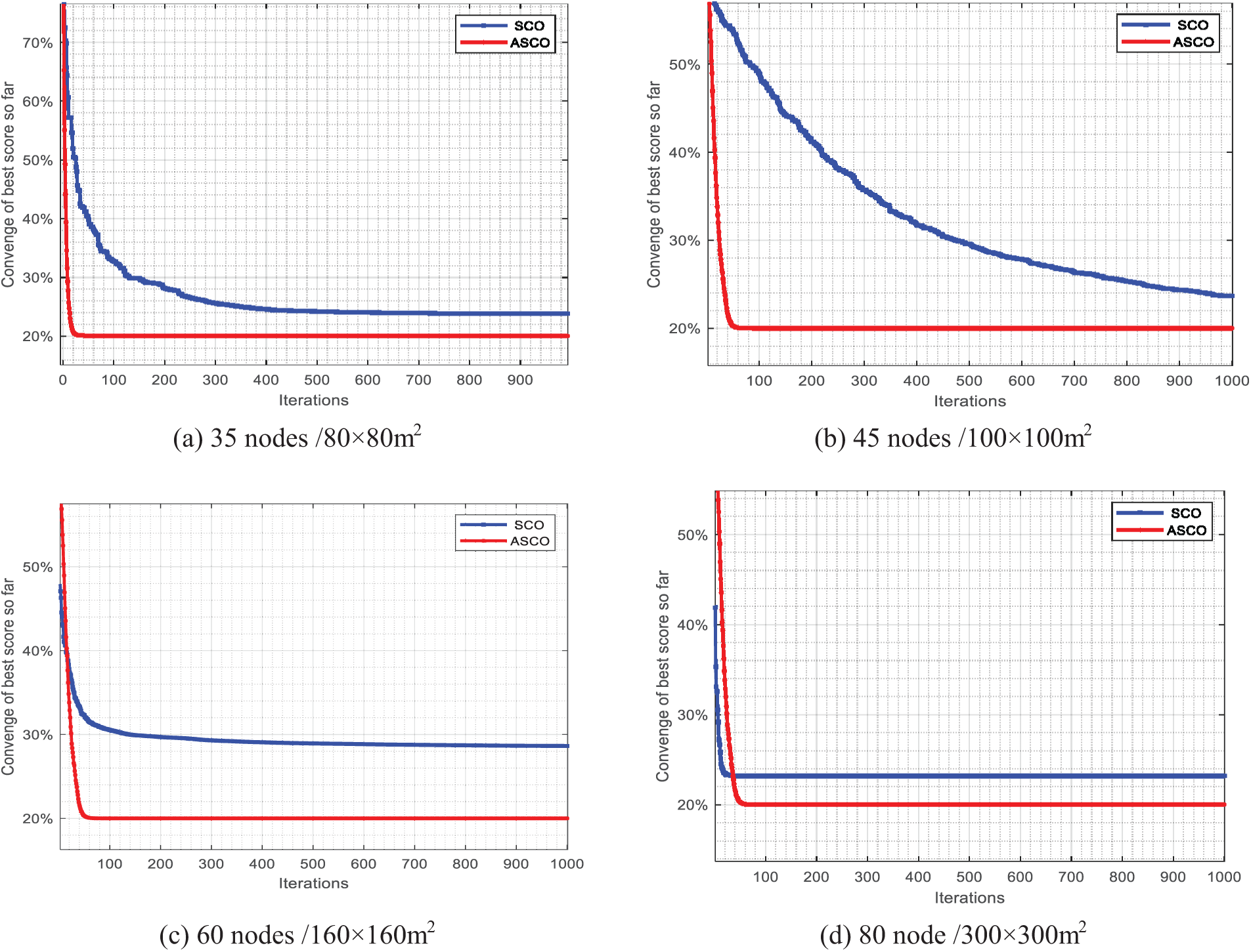
Figure 2: Comparison of the ASCO’s graphical coverage diagram with the original SCO for the statistical coverage optimization scheme with various density nodes: (a) 35 nodes/80 × 80 m2,(b) 45 nodes/100 × 100 m2, (c) 60 nodes/160 × 160 m2, and (d) 80 nodes/300 × 300 m2, respectively

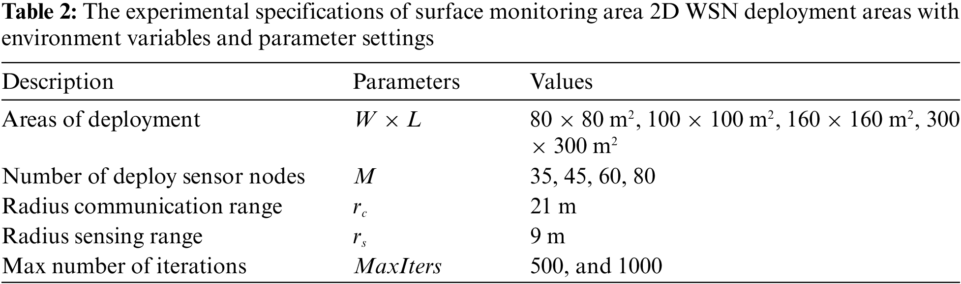
The experimental specifications of WSN deployment areas with environment variables and parameter settings are used for testing the validated performance and accuracy of the suggested approach, as shown in Table 2. The optimal statistical coverage in scheme’s initialization graphical coverage planning phase for the ASCO which is with M set to 35, 45, 60, and 80 nodes, respectively. Fig. 3 shows the initialization graphical node coverages of the ASCO for the statistical coverage optimization scheme with M set to 35, 45, 60, and 80, respectively.

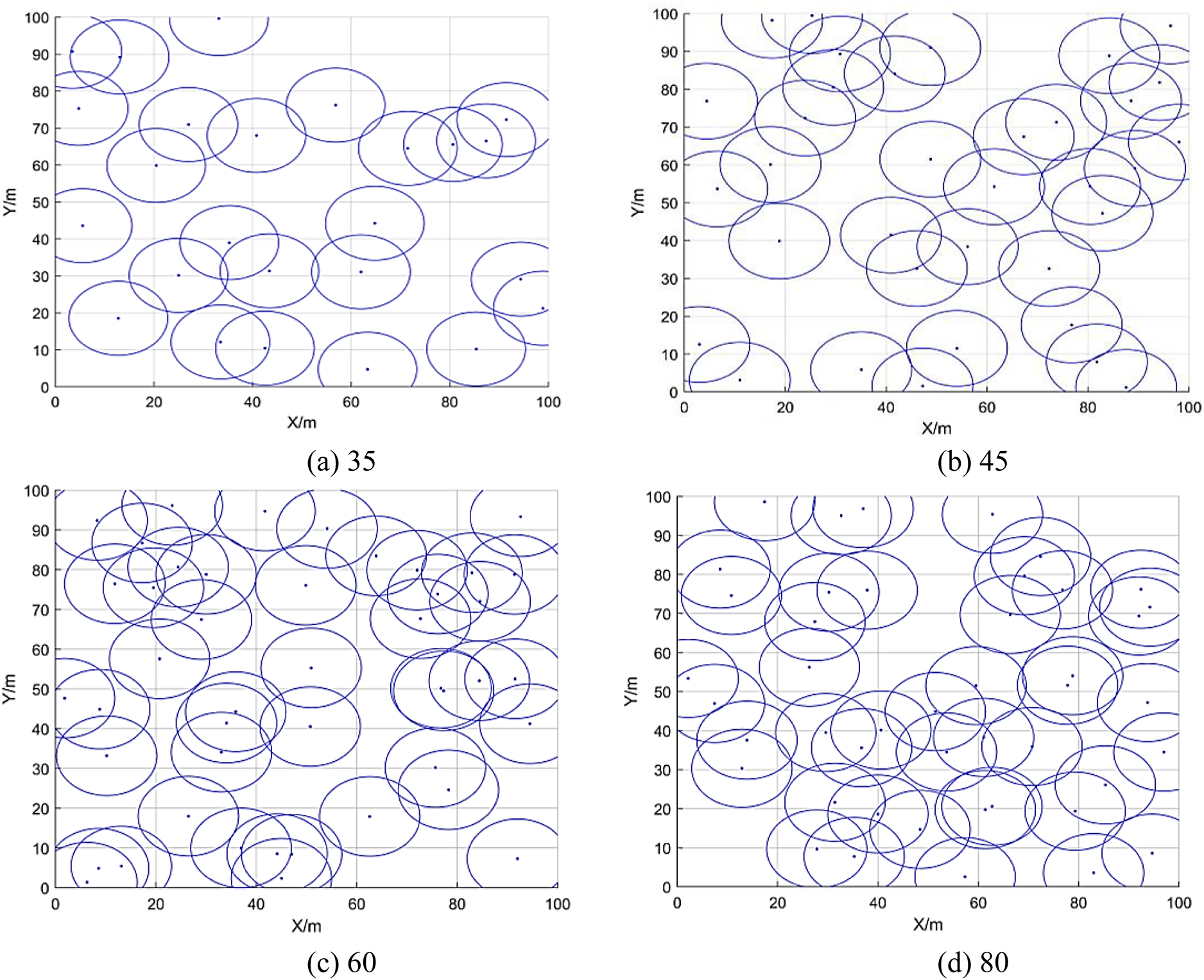
Figure 3: The initialization graphical nodes in network deployment for the optimal statistical coveragea planning with various M sets of the number of sensor nodes set to, respectively, (a) 35, (b) 45, (c) 60, and (d) 80

Fig. 4 shows a graphical convergence comparision of the ASCO scheme with different metaheuristic algorithms, e.g., the SSA [42], PSO [43], GWO [44], SCA [45], and SCO [38] approaches for the WSN node areas deployment scenarios for optimal coverage rates with the density and condition environment setting, such as (a) 35/80 × 80 m2, (b) 45/100 × 100 m2, (c) 60/160 × 160 m2, and (d) 80/300 × 300 m2, respectively. The experimental implementation scenarios of the metaheuristic methods for four different sizes of WSN monitoring node areas are shown in Fig. 4 for the best coverage rates. It compares the ASCO optimization in terms of convergence speeds for deployment coverage rate against the SSA, PSO, GWO, SCA, and SCO algorithms. As can be seen, the ASCO algorithm produces the curves of a convergence rate in the network coverage of the monitoring area that is relatively high. In some circumstances, the suggested ASCO approach’s convergence curves can offer larger static coverage percentages than the competing approaches.

Figure 4: Several scenarios for deploying WSN monitoring node areas of various sizes for the best coverage rates, e.g., (a) 35/80 × 80 m2, (b) 45/100 × 100 m2, (c) 60/160 × 160 m2, and (d) 80/300 × 300 m2

Table 3 compares the percentage coverage rate, running times, convergence iterations, and monitoring area sizes of the proposed ASCO approach to other approaches, such as the SSA [42], PSO [43], GWO [44], SCA [45], MIGA [41], and SCO [38] algorithms. Because the ASCO algorithm has adapted its solution for initializing, exploiting, and exploring directions that can avoid premature phenomena, the coverage rate is reasonably high. The results show that the ASCO algorithm provides a relatively high coverage rate with less overlap and a better-altered layout of the sensor nodes under the same test conditions. It is clear that the ASCO scheme, which has a high coverage rate, complete coverage of the node’s space area, and a quicker time consumption than the other approaches, produces the best overall solution in the coverage areas.

Fig. 5 presents the graphical coverages of the ASCO approach and various metaheuristic algorithms, e.g., SCO, PSO, GWO, SCA, and SSA for WSN deploying areas. A precise observation from the graph is that the ASCO approach outperforms the other approaches regarding coverage.

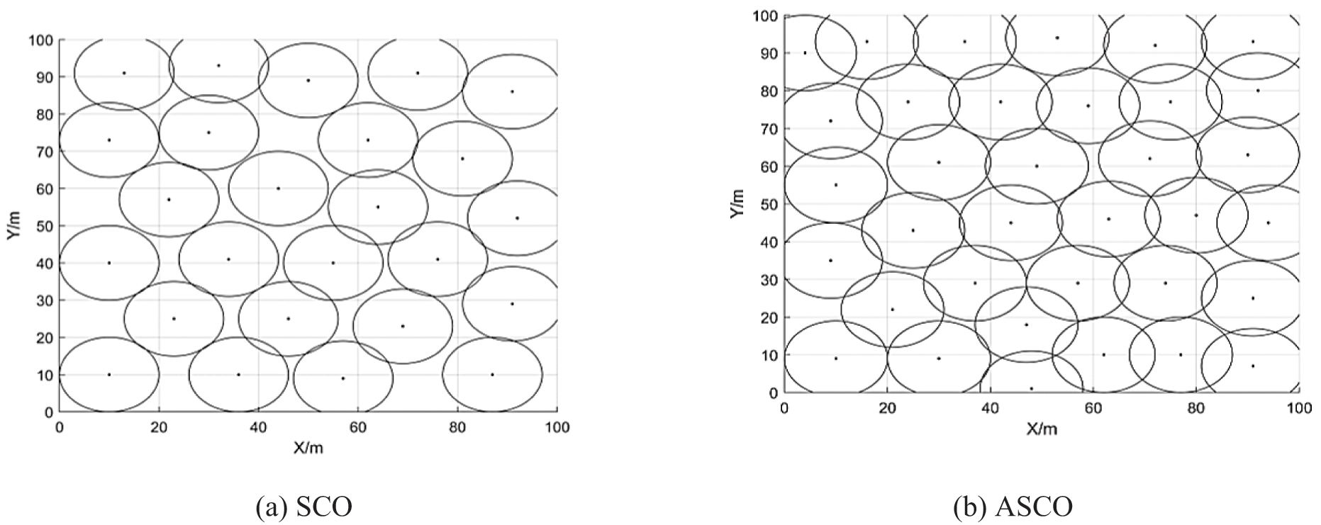
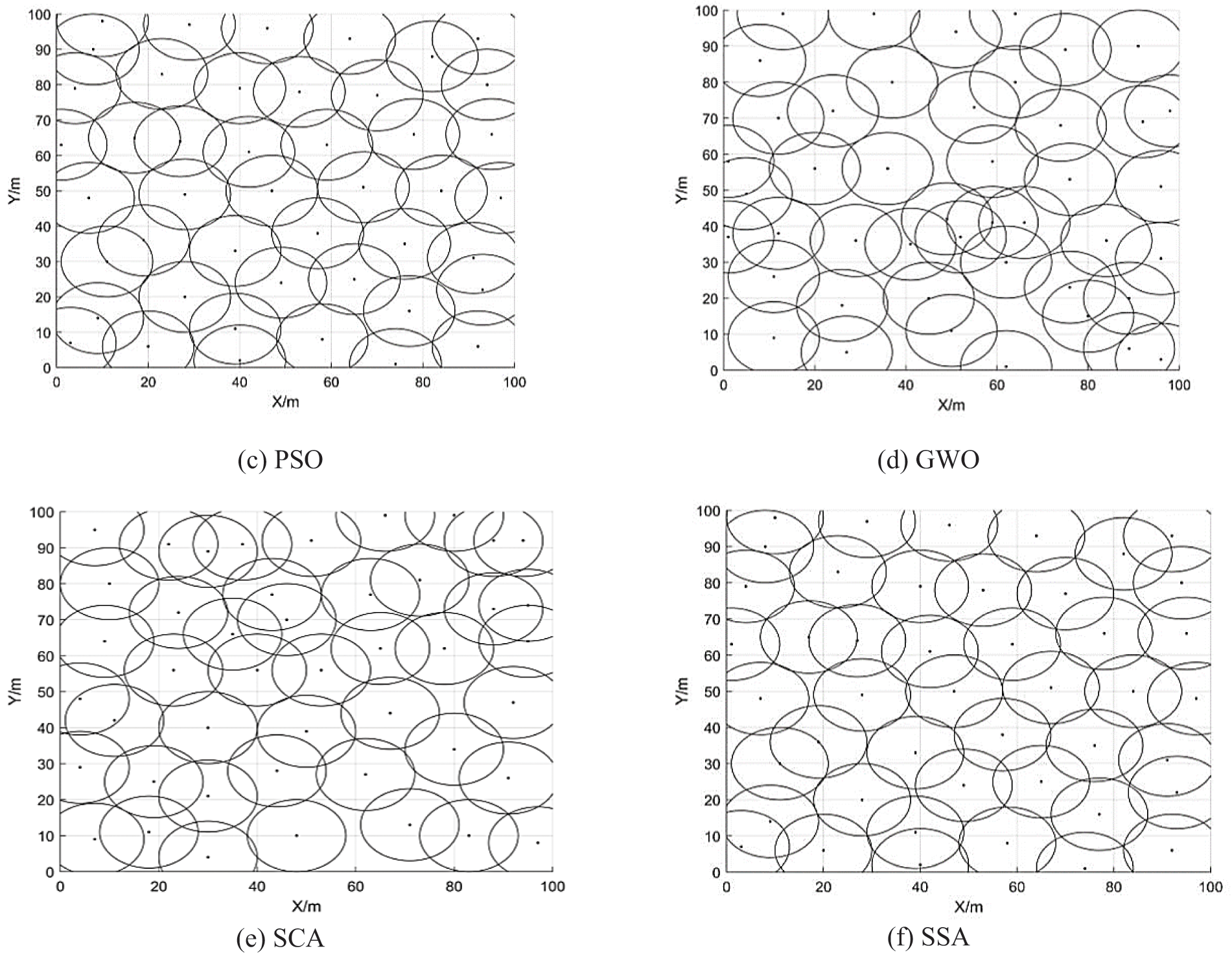
Figure 5: The obtained results as graphical coverages of the ASCO approach and the metaheuristic algorithms, such as the SCO [38], PSO [43], GWO [44], SCA [45], and SSA [42] for the WSN deploying areas

The various scenarios are carried out in the 2D monitoring areas. Fig. 6 compares the ASCO optimization’s statistical sensor node counts deployment coverage rate against the SCO, SCA, GWO, PSO, and SSA algorithms. As can be seen in the chart bars of the figure, the ASCO algorithm delivers a coverage rate in the network coverage of the monitoring area that is relatively high. The results show that the ASCO technique provides a relatively high coverage rate with less overlap and a better-altered layout of the sensor nodes under the same test conditions. The node’s configuration in the applied ASCO scheme was better adapted than its competitors for the monitoring area’s network coverage.

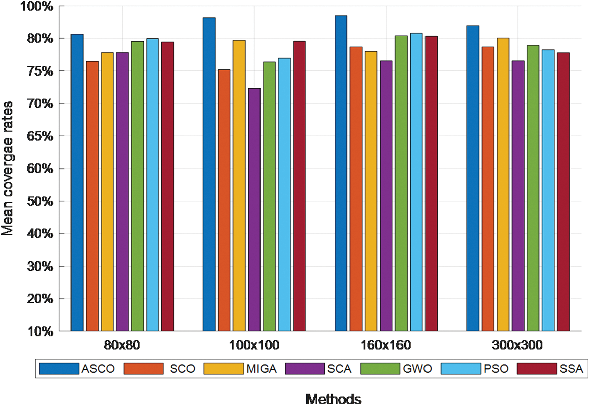
Figure 6: A comparison of the ASCO optimization’s statistical sensor node counts deployment coverage rate against the SCO, MIGA, SCA, GWO, PSO, and SSA algorithms for different sensor node counts deployed on the 2D monitoring areas

5  Conclusion

This study suggested improved strategies for the adjusted single candidate optimizer (ASCO) due to the limited ability of the original single candidate optimizer (SCO) to deal with the complicated issues of low WSN coverage and nodes’ uneven distribution in the random deployment. We carried out the ASCO scheme by changing equations for updating candidate solutions with apposite learning and multi-direction tactics to avoid the shortcomings of the original single candidate optimizer approach—such as its slow convergence speed and ease of sliding into local extrema. When deploying WSN, the fitness function of the ideal node coverage is mathematically modeled by estimating the distance between nodes by evaluating each sensor node’s sensing radius and communication capabilities. The network coverage with the applied ASCO effectively provides the best solution to coverage issues, according to optimal findings on the WSN node coverage. The ASCO’s optimal coverage test results were compared to other algorithms in the literature. The compared results demonstrate that the ASCO algorithm offers efficient, optimal performance, rapid convergence, and expanding realizable coverage. Significantly, the ASCO’s archival coverage rate is 89%, while the other approaches only achieve coverage rates below or equal to 84% when compared under the same conditions. In future work, the focus will expand beyond coverage optimization to encompass additional challenges in WSN deployments. One such challenge is node localization, which will be addressed by applying the ASCO scheme. Furthermore, the research scope will extend to include WSN deployments in non-uniform or complex terrains, where node distribution and environmental conditions can vary significantly.

Acknowledgement: The authors thank the anonymous reviewers for their insightful comments and suggestions on improving this paper.

Funding Statement: This study was partially supported by the VNUHCM-University of Information Technology’s Scientific Research Support Fund.

Conflicts of Interest: The authors declare that they have no conflicts of interest to report regarding the present study.

References

1. G. Fan and S. Jin, “Coverage problem in wireless sensor network: A survey,” Journal of Networks, vol. 5, no. 9, pp. 1033–1040, 2010. [Google Scholar]

2. J. Yick, B. Mukherjee and D. Ghosal, “Wireless sensor network survey,” Computer Networks, vol. 52,no. 12, pp. 2292–2330, 2008. [Google Scholar]

3. G. Usha, S. Kannimuthu, P. D. Mahendiran, A. K. Shanker and D. Venugopal, “Static analysis method for detecting cross site scripting vulnerabilities,” International Journal of Information and Computer Security, vol. 13, no. 1, pp. 32–47, 2020. [Google Scholar]

4. T. T. Nguyen, C. S. Shieh, T. K. Dao, J. S. Wu and W. C. Hu, “Prolonging of the network lifetime of WSN using fuzzy clustering topology,” in Proc. of 2013 2nd Int. Conf. on Robot, Vision and Signal Processing, RVSP, Kaoshiung, Taiwan, pp. 13–16, 2013. [Google Scholar]

5. K. S. Adu-Manu, N. Adam, C. Tapparello, H. Ayatollahi and W. Heinzelman, “Energy-harvesting wireless sensor networks (EH-WSNsA review,” ACM Transactions on Sensor Networks, vol. 14, no. 2, pp. 1–50, 2018. [Google Scholar]

6. S. Balachandran Nair Premakumari, P. Mohan and K. Subramanian, “An enhanced localization approach for energy conservation in wireless sensor network with Q deep learning algorithm,” Symmetry, vol. 14, no. 12, pp. 2515, 2022. https://doi.org/10.3390/sym14122515 [Google Scholar] [CrossRef]

7. S. G. Shiva Prasad Yadav and A. Chitra, “Wireless sensor networks—Architectures, protocols, simulators and applications: A survey,” International Journal of Electronics and Computer Science Engineering, vol. 1, no. 4, pp. 1941–1953, 2012. [Google Scholar]

8. U. Gopal and K. Subramanian, “A secure cross-layer AODV routing method to detect and isolate (SCLARDI) black hole attacks for MANET,” Turkish Journal of Electrical Engineering and Computer Sciences, vol. 25, no. 4, pp. 2761–2769, 2017. [Google Scholar]

9. A. K. Dwivedi and A. K. Sharma, “I-FBECS: Improved fuzzy based energy efficient clustering using biogeography based optimization in wireless sensor network,” Transactions on Emerging Telecommunications Technologies, vol. 32, no. 2, pp. 1–17, 2021. [Google Scholar]

10. T. K. Dao, S. C. Chu, T. T. Nguyen, T. D. Nguyen and V. T. Nguyen, “An optimal WSN node coverage based on enhanced archimedes optimization algorithm,” Entropy, vol. 8, no. 24, pp. 1018, 2022. https://doi.org/10.3390/e24081018 [Google Scholar] [PubMed] [CrossRef]

11. A. K. Dwivedi and A. K. Sharma, “EE-LEACH: Energy enhancement in LEACH using fuzzy logic for homogeneous WSN,” Wireless Personal Communications, vol. 120, no. 4, pp. 3035–3055, 2021. [Google Scholar]

12. T. Dao, J. Yu, T. Nguyen and T. Ngo, “A hybrid improved MVO and FNN for Identifying collected data failure in cluster heads in WSN,” IEEE Access, vol. 8, pp. 124311–124322, 2020. [Google Scholar]

13. M. F. Othman and K. Shazali, “Wireless sensor network applications: A study in environment monitoring system,” Procedia Engineering, vol. 41, pp. 1204–1210, 2012. [Google Scholar]

14. M. Li and B. Yang, “A survey on topology issues in wireless sensor network,” in Int. Conf. on Wireless Networks, ICWN 2006, Las Vegas, Nevada, USA, no. 503, 2006. [Google Scholar]

15. A. K. Dwivedi, A. K. Sharma and P. S. Mehra, “Energy efficient sensor node deployment scheme for two stage routing protocol of wireless sensor networks assisted IoT,” ECTI Transactions on Electrical Engineering, Electronics, and Communications, vol. 18, no. 2, pp. 158–169, 2020. [Google Scholar]

16. S. C. Chu, T. K. Dao, J. S. Pan and T. T. Nguyen, “Identifying correctness data scheme for aggregating data in cluster heads of wireless sensor network based on Naive Bayes classification,” EURASIP Journal on Wireless Communications and Networking, vol. 2020, no. 1, pp. 1–15, 2020. [Google Scholar]

17. T. T. Nguyen, J. S. Pan and T. K. Dao, “An improved flower pollination algorithm for optimizing layouts of nodes in wireless sensor network,” IEEE Access, vol. 7, pp. 75985–75998, 2019. [Google Scholar]

18. T. T. Nguyen, T. K. Dao, H. Y. Kao, M. F. Horng and C. S. Shieh, “Hybrid particle swarm optimization with artificial bee colony optimization for topology control scheme in wireless sensor networks,” Journal of Internet Technology, vol. 18, no. 4, pp. 743–752, 2017. [Google Scholar]

19. T. T. Nguyen, T. K. Dao, M. F. Horng and C. S. Shieh, “An energy-based cluster head selection algorithm to support long-lifetime in wireless sensor networks,” Journal of Network Intelligence, vol. 1, no. 1, pp. 23–37, 2016. [Google Scholar]

20. J. S. Pan, T. T. Nguyen, S. C. Chu, T. K. Dao and T. G. Ngo, “Diversity enhanced ion motion optimization for localization in wireless sensor network,” Journal of Information Hiding and Multimedia Signal Processing, vol. 10, no. 1, pp. 221–229, 2019. [Google Scholar]

21. B. Wang, “Coverage problems in sensor networks: A survey,” ACM Computing Surveys (CSUR), vol. 43, no. 4, pp. 1–53, 2011. [Google Scholar]

22. I. F. Akyildiz, W. Su, Y. Sankarasubramaniam and E. Cayirci, “Wireless sensor networks: A survey,” Computer Networks, vol. 38, no. 4, pp. 393–422, 2002. [Google Scholar]

23. A. K. Dwivedi, P. S. Mehra, O. Pal, M. N. Doja and B. Alam, “EETSP: Energy-efficient two-stage routing protocol for wireless sensor network-assisted Internet of Things,” International Journal of Communication Systems, vol. 34, no. 17, pp. e4965, 2021. [Google Scholar]

24. T. K. Dao, T. S. Pan, T. T. Nguyen and S. C. Chu, “A compact articial bee colony optimization for topology control scheme in wireless sensor networks,” Journal of Information Hiding and Multimedia Signal Processing, vol. 6, no. 3, pp. 297–310, 2015. [Google Scholar]

25. N. A. B. A. Aziz, A. W. Mohemmed and M. Y. Alias, “A wireless sensor network coverage optimization algorithm based on particle swarm optimization and Voronoi diagram,” in 2009 Int. Conf. on Networking, Sensing and Control, Okayama, Japan, pp. 602–607, 2009. [Google Scholar]

26. A. K. Dwivedi and A. K. Sharma, “FEECA: Fuzzy based energy efficient clustering approach in wireless sensor network,” EAI Endorsed Transactions on Scalable Information Systems, vol. 7, no. 27, pp. e5, 2020. [Google Scholar]

27. A. K. Dwivedi and A. K. Sharma, “NEEF: A novel energy efficient fuzzy logic based clustering protocol for wireless sensor network,” Scalable Computing: Practice and Experience, vol. 21, no. 3, pp. 555–568, 2020. [Google Scholar]

28. T. T. Nguyen, J. S. Pan, T. K. Dao, T. W. Sung and T. G. Ngo, “Pigeon-inspired optimization for node location in wireless sensor network,” in Advances in Engineering Research and Application, vol. 104. Thai Nguyen Vietnam: ICERA, 2020. [Google Scholar]

29. T. T. Nguyen, J. S. Pan, J. C. W. Lin, T. K. Dao and T. X. H. Nguyen, “An optimal node coverage in wireless sensor network based on whale optimization algorithm,” Data Science and Pattern Recognition, vol. 2, no. 2, pp. 11–21, Saigon, Vietnam, 2018. [Google Scholar]

30. R. V. Kulkarni and G. K. Venayagamoorthy, “Particle swarm optimization in wireless-sensor networks: A brief survey,” IEEE Transactions on Systems, Man, and Cybernetics, Part C (Applications and Reviews), vol. 41, no. 2, pp. 262–267, 2010. [Google Scholar]

31. Z. Tian and S. Fong, “Survey of meta-heuristic algorithms for deep learning training,” in Optimization Algorithms—Methods and Applications. London, UK: IntechOpen, pp. 195–220, 2016. [Google Scholar]

32. Z. Beheshti and S. M. H. Shamsuddin, “A review of population-based meta-heuristic algorithm,” International Journal of Advances in Soft Computing and its Applications, vol. 5, no. 1, pp. 1–35, 2013. [Google Scholar]

33. T. K. Dao, T. T. Nguyen, V. T. Nguyen and T. D. Nguyen, “A hybridized flower pollination algorithm and its application on microgrid operations planning,” Operations Planning, Applied Sciences, vol. 12,no. 13, pp. 6487, 2022. [Google Scholar]

34. R. Alkanhel, K. Chinnathambi, C. Thilagavathi, M. Abouhawwash, A. Al duailij et al., “An energy-efficient multi-swarm optimization in wireless sensor networks,” Intelligent Automation & Soft Computing, vol. 36, no. 2, pp. 1571–1583, 2023. [Google Scholar]

35. M. Srinivas and L. M. Patnaik, “Genetic algorithms: A survey,” Computer, vol. 27, no. 6, pp. 17–26, 1994. [Google Scholar]

36. Y. Shi and R. Eberhart, “A modified particle swarm optimizer,” in IEEE Int. Conf. on Evolutionary Computation, Anchorage, AK, USA, pp. 69–73, 1998. [Google Scholar]

37. E. Rashedi, H. Nezamabadi-Pour and S. Saryazdi, “GSA: A gravitational search algorithm,” Information Sciences, vol. 179, no. 13, pp. 2232–2248, 2011. [Google Scholar]

38. T. M. Shami, D. Grace, A. Burr and P. D. Mitchell, “Single candidate optimizer: A novel optimization algorithm,” Evolutionary Intelligence, vol. 3, no. 1, pp. 1, 2022. https://doi.org/10.1007/s12065-022-00762-7 [Google Scholar] [CrossRef]

39. M. Farsi, M. A. Elhosseini, M. Badawy, H. A. Ali and H. Z. Eldin, “Deployment techniques in wireless sensor networks, coverage and connectivity: A survey,” IEEE Access, vol. 7, pp. 28940–28954, 2019. [Google Scholar]

40. D. K. Chaudhary and R. L. Dua, “Application of multi objective particle swarm optimization to maximize coverage and lifetime of wireless sensor network,” International Journal of Computer Engineering Research, vol. 2, pp. 1628–1633, 2012. [Google Scholar]

41. N. T. Hanh, H. T. T. Binh, N. X. Hoai and M. S. Palaniswami, “An efficient genetic algorithm for maximizing area coverage in wireless sensor networks,” Information Sciences, vol. 488, no. 6, pp. 58–75, 2019. [Google Scholar]

42. J. Chelliah and N. Kader, “Optimization for connectivity and coverage issue in target-based wireless sensor networks using an effective multiobjective hybrid tunicate and salp swarm optimizer,” International Journal of Communication Systems, vol. 34, no. 3, pp. 1–17, 2021. [Google Scholar]

43. W. T. Liu and Z. Y. Fan, “Coverage optimization of wireless sensor networks based on chaos particle swarm algorithm,” Journal of Computer Applications, vol. 31, no. 2, pp. 338–340, 2011. [Google Scholar]

44. Z. Wang, H. Xie, Z. Hu, D. Li, J. Wang et al., “Node coverage optimization algorithm for wireless sensor networks based on improved grey wolf optimizer,” Journal of Algorithms & Computational Technology,vol. 13, pp. 1–15, 2019. [Google Scholar]

45. F. Fan, S. C. Chu, J. S. Pan, Q. Yang and H. Zhao, “Parallel sine cosine algorithm for the dynamic deployment in wireless sensor networks,” Journal of Internet Technology, vol. 22, no. 3, pp. 499–512, 2021. [Google Scholar]

46. T. T. Nguyen, J. S. Pan, T. Y. Wu, T. K. Dao and T. D. Nguyen, “Node coverage optimization strategy based on ions motion optimization,” Journal of Network Intelligence, vol. 4, no. 1, pp. 1–9, 2019. [Google Scholar]