Loss Factors and their Effect on Resonance Peaks in Mechanical Systems

1  Introduction

Careful work is required to optimize the quality and reliability of engineering projects. It is not easy to develop things right the first time, and much effort is spent on corrective actions. One of the main problems is a lack of true understanding of the physical effects and parameters. Many engineers used to offer immediate practical solutions, rather than performing preliminary theoretical analysis. So did Thomas Edison, the great inventor who persistently applied the “trial and error” method to his work. But a purely empiric approach does not guarantee positive results. Nikola Tesla, another great inventor, was “a sorry witness” to Edison’s procedure, “knowing that just a little theory and calculation would have saved him ninety per cent of the labor”.

On the other hand, accurate theoretical models may look complicated. Even computer modeling may not fully compensate for this shortage. This is why brief reviews and tutorials are highly helpful for practical engineers engaged in design, testing, and manufacture.

This paper is devoted to the mechanical loss factor which controls the magnitudes and frequencies of resonance peaks in vibration and acoustical phenomena. In this paper, some well-known aspects are clarified for practitioners, and some results are new.

The mechanical loss factor may depend on (1) the energy dissipation capacity of materials, (2) geometric, inertial, and elastic properties of the whole construction, (3) vibration energy dissipation in the links between the construction and adjacent structures, (4) vibration transmission into adjacent structures, and (5) sound radiation into an ambient gas or liquid medium [1–6]. It can be also affected by the ambient temperature and other physical phenomena (in particular, by electrostatic phenomena in MEMS). The resonance effects sometimes look complicated but even a general theoretical knowledge helps avoiding serious errors in the engineering projects.

The paper is addressed to the design, analysis and test engineers engaged in noise, vibration, and vibration fatigue control (in particular, NVH engineers). The possible applications are multiple: building structures, automotive and aerospace vehicles, rotating machinery, fans and blowers, microelectromechanical systems (MEMS), etc.

2  Definition of Mechanical Loss Factor

For a vibrating system excited by a steady-state harmonic force, the mechanical loss factor is defined as

η=D2πℰ (1)

where ℰ is the total vibration energy of the system, and D is the vibration energy dissipated per cycle which is equivalent to the vibration energy input; hence, the value D/(2π) is the average energy loss per radian [1–3]. Commonly, the loss factor η << 1 but theoretically it can exceed 1. The latter is not in contradiction with the law of conservation of energy since the internal energy loss is partly compensated by the continuous energy input from outside.

There are three prime parts in the lumped mechanical models: rigid mass, massless spring, and dashpot, or viscous damper. We may call them elements because each of them represents only one physical property: the mass simulates inertia, the spring controls elastic deformation, and the dashpot symbolizes velocity-proportional energy dissipation of the vibration elements.

Express the Eq. (1) in terms of mass m, stiffness k, and viscous damper coefficient c of the Kelvin-Voight model (Fig. 1a) which represents the classic linear 1-DOF (single-degree-of-freedom) viscoelastic system. In this case, the elastic and viscous forces can be expressed respectively as Fe=kx=kAcos(ωt) and Fv=cx˙=−kωAsin(ωt) where the vibration displacement x(t)=Acos(ωt) . Here, ω=2πf is the angular frequency and f is the frequency of vibration. If  x˙(0)=0 , the total vibration energy equals the initial elastic energy:

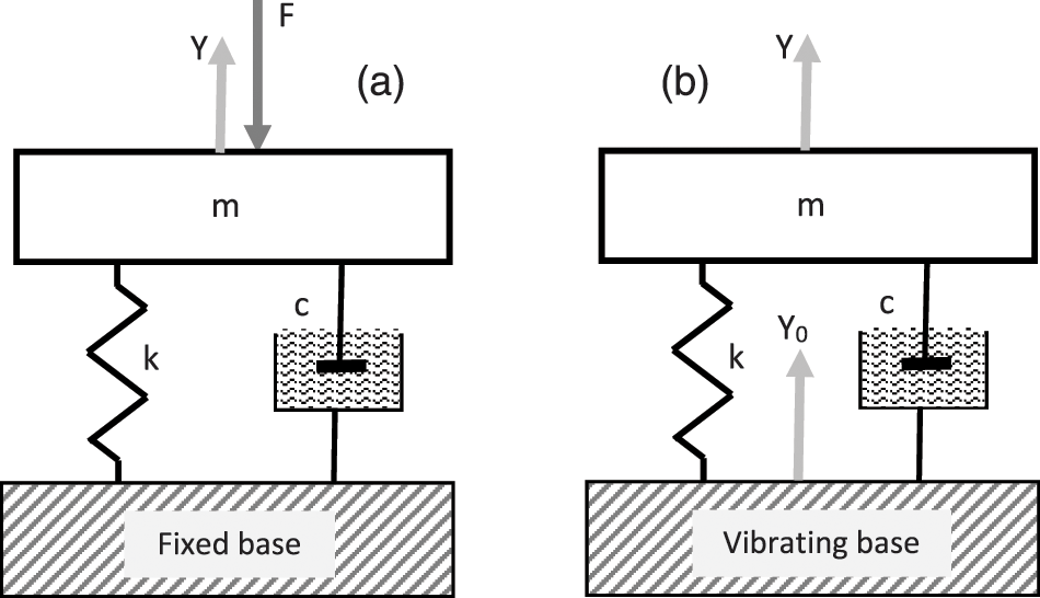
Figure 1: Classic (a) and NVH (b) 1-DOF linear models of mechanical vibration systems

ℰ=kx(0)22=kA22.

The vibration energy dissipated per each cycle calculates

D=∫0T⁡Fvx˙dt=cA2ω∫02π⁡[sin⁡(ωt)]2d(ωt)=π cA2ω

where T=2π/ω is the period of vibration.

Substituting the expressions for ℰ and D into Eq. (1), obtain

η=cωk=cmkωω0 (2)

where the angular undamped natural frequency of the system

ω0=k/m . (3)

Commonly, the damped (resonance) and undamped natural frequencies of 1-DOF systems are close to each other as shown in Chapter 3.5 (this may not be true for 2-DOF systems, see Chapter 4.4). Then, as follows from Eq. (3), the loss factor of 1-DOF system at the resonance frequency may be given as

η≈ckm . (4)

Basing upon the classic 1-DOF model, two general conclusions can be made:

1.    The mechanical loss factor depends on both inertial, elastic, and energy dissipation parameters of vibrating systems.

2.    Under the same energy dissipation ability, the lower the system stiffness and mass, the higher the loss factor. This trend is observed in many practical cases.

3  Loss Factor of 1-DOF System

3.1 Classic Model of 1-DOF System

In the classic model of 1-DOF system (Fig. 1a), the spring and dashpot are linear, that is, the elastic and viscous forces are proportional respectively to the displacement and velocity. Such approximations are reasonable for the most practical cases though (1) the real dissipation mechanisms may be nonlinear (in particular, dry friction or hysteresis), and (2) the famous Hooke’s Law of Elasticity, is fully relevant only to linear-elastic or “Hookean” materials.

The differential equation of steady-state harmonic motion is

m x¨ +  cx˙+kx=Feiωt (5)

where F is the amplitude of an external harmonic force, and the system parameters are described in Chapter 2. The solution of Eq. (5) is x=Aeiωt .

Therefore x˙=iωAeiωt=iωx. Substituting this relationship into Eq. (5) and using Eq. (2), obtain

m x¨+k˜x=Feiωt (6)

where the complex stiffness

k~=k(1+iη). (7)

The solution of Eq. (6) is

x(t)=Fk eiωt1−(ω/ω0)2+iη (8)

where ω0 is defined by Eq. (3).

3.2 NVH Model of 1-DOF System

This model is similar to the classic model of 1-DOF system except for the excitation way: it is driven by a harmonically moving base attached to the spring (Fig. 1b). It may be mentioned as the NVH model since the vibrating base may simulate a shaker head on NVH testing.

Here, the differential equation of steady-state motion is similar to Eq. (6) for the relevant classic model if the force amplitude is expressed in the form F=k~ x0 where  x0=Beiωt describes the base displacement.

Using Eq. (8), one can derive the expression for vibration transmissibility (the module of the ratio of the mass movement to the base movement).

T=|xx0|= 1+η2{1−(ω/ω0)2}2+η2 ≈1{1−(ω/ω0)2}2+η2 (9)

3.3 Free-Damped Vibration of 1-DOF System

The amplitude of steady-state vibration does not change with time because the outside input energy equals the energy dissipation inside the system. But there is no input energy in case of damped free vibration, and the amplitude decays with time.

Free harmonic vibration of 1-DOF system starts as soon as the external force is off. This motion, described by Eq. (5) in case F=0 , can be given by

x=x0 e−ζω0t+iω01−ζ2 t (10)

where x0 is the initial displacement amplitude and the initial velocity equals zero.

Here, the well-known damping ratio

ζ=c/(2km )= η/2   (11)

where η is the loss factor given by Eq. (4).

As shown, the relationship (11) between the damping ratio and loss factor is quite simple. This is important to know because two wrong opinions are shared by some practical engineers: (1) the damping ratio and loss factor are the same parameters, (2) not the same parameters but the relationship between them is quite cumbersome.

It is also important to remember that the damping ratio is defined just in case of viscous friction, while the loss factor exists for any type of vibration energy dissipation.

As follows from Eq. (10), the free-damped vibration amplitude changes in time as exponentially decaying function if ζ<1 , or, as follows from Eq. (11), η<2 . In most practical cases, the loss factors are much lower (mainly between 0.01 and 0.10). However, the loss factors of some special structural elements (in particular, vibration isolation mounts) can be up to 0.3 and even higher.

3.4 Correct Sign for Imaginary Part of the Complex Modulus of Elasticity

The complex modulus of elasticity is commonly defined as

E∗=E(1+iη) (12)

where E is the real modulus of elasticity [1–3]. For solid structures, the stiffness k is proportional to modulus of elasticity E , so, Eq. (7) directly follows from Eq. (12).

It should be noted that in some old publications, the complex modulus of elasticity is defined with the negative imaginary part:

E∗=E(1−iη). (13)

The difference between Eqs. (12) and (13) is critical in mathematical modeling. As shown in paper [7], Eq. (12) is correct if the time-oscillating factor in the equations of motion is eiωt , and Eq. (13) is correct if the time-oscillating factor is e−iωt . If Eqs. (12) and (13) are used with the oscillating factors e−iωt and eiωt , respectively, the energy conservation law is violated. Certainly, the same holds true for the complex stiffnesses.

This important issue is not mentioned in the standard [1] and most engineering textbooks. The reason can be the following: Eqs. (12) or (13) are just symbolic for practical engineers who are not directly engaged in mathematical modeling.

3.5 Effect of Loss Factor on the Resonance Frequency of 1-DOF System

The peak frequency response of 1-DOF vibration system occurs at its resonance frequency fr (also known as the damped natural frequency) which coincides with the undamped natural frequency f0 only if the loss factor is independent of frequency [2,4]. Otherwise, the resonance and undamped natural frequencies differ. Sometimes, this becomes a matter of disputation among engineers (what frequency is greater and how much). In most publications, the relationship between the two is analyzed just for viscous damping.

But the loss factors can be created by various energy dissipation mechanisms. Generally, in the narrow vicinity of the undamped natural frequency, the loss factor may be described by a power function

η=βfp

where β is a constant value, f is the frequency and parameter p depends on the type of energy dissipation. Therefore, as shown in paper [8], the ratio of the resonance frequency fr and undamped natural frequency f0 can be expressed as

frf0=1−pη4 . (14)

There are three important cases:

1.     p=1 for viscous friction or airborne sound radiation,

2.     p=0 for hysteresis type of internal friction in solids,

3.     p=−1/2 for structural energy losses (see Chapter 6).

Thus, as follows from Eq. (14), the resonance frequency may slightly exceed (for structural energy losses), equal (for hysteretic friction), or slightly fall below the undamped natural frequency (for viscous friction). Even for the relatively high loss factor η=0.2 , the ratio fr/f0 calculates close to 1: 0.95, 1.00, and 1.025, respectively. This trend is graphically illustrated in Fig. 2.

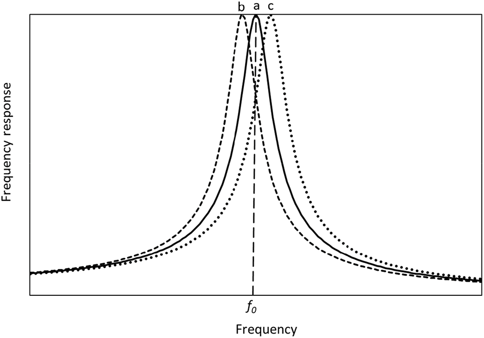
Figure 2: Typical frequency responses for 1-DOF models with the same undamped natural frequency f0 and various damping mechanisms: (a) hysteresis, (b) viscous friction, (c) structural damping

In most practical cases, hysteretic damping is acceptable for mathematical models because the real loss factors do not much change within relatively narrow frequency intervals (in particular, near the resonance frequencies).

3.6 Loss Factor in Micro Electromechanical Systems (MEMS). Negative Spring and Squeeze-Film Effects

MEMS technology combines micromachining with microelectronics and is widespread in aerospace, automotive, biological/medical, military, and photonics applications. A typical MEMS design incorporates a microsensor (accelerometer, load cell, microphone, etc.), micro actuator (lever, gear, micro-mirror, valve, pump, motor, etc.), processor chip, and package. The size of micro transducers (microsensors and micro actuators) is commonly within millimeters or even microns. The conventional electrostatic parallel-plate model of a capacitive sensor includes a narrow air film between the plates where one of the plates plays the role of mechanical mass and the other plate is fixed.

There are two important effects influencing the loss factor of this system: the squeeze-film damping and negative spring effect [9,10].

The moving plate’s displacement squeezes air in and out of the gap, and the relevant viscosity force can be significant since the air film is very thin. Besides, the mass of the moving plate is rather small. For such two reasons, as follows from Eq. (4), the loss factor gets high values and therefore impedes the plate movement. The squeeze-film effect can be mitigated via reducing air pressure in the gap to very low values (to the condition of molecular slip flow when the mean-free molecular path gets smaller than the air gap). In this case, the air molecules strike the plates rather than other air molecules, and the viscous friction becomes insignificant.

The negative spring effect is caused by the elastic and electrostatic force acting in the opposite directions. Thus, the effective stiffness of the system is lower than the elastic stiffness. As follows from Eq. (4), such a difference increases the loss factor.

4  Loss Factors of 2-DOF in-Series System with Hysteretic Friction

4.1 Equations of Motion for 2-DOF in-Series System with Vibrating Base (NVH Model)

Both classic and NVH 2-DOF in-series mechanical systems (Figs. 3a and 3b) are important for engineering applications. Let’s discuss the NVH model with a harmonically vibrating base, two masses and two springs with internal hysteretic damping (Fig. 3b). The elements are arranged in the following order: vibrating rigid base—first dampened spring—first mass—second dampened spring—second mass. Such a construction includes two in-series 1-DOF systems: (1) the main subsystem, consisting of the first spring and the first mass, and (2) auxiliary subsystem including the second spring and the second mass.

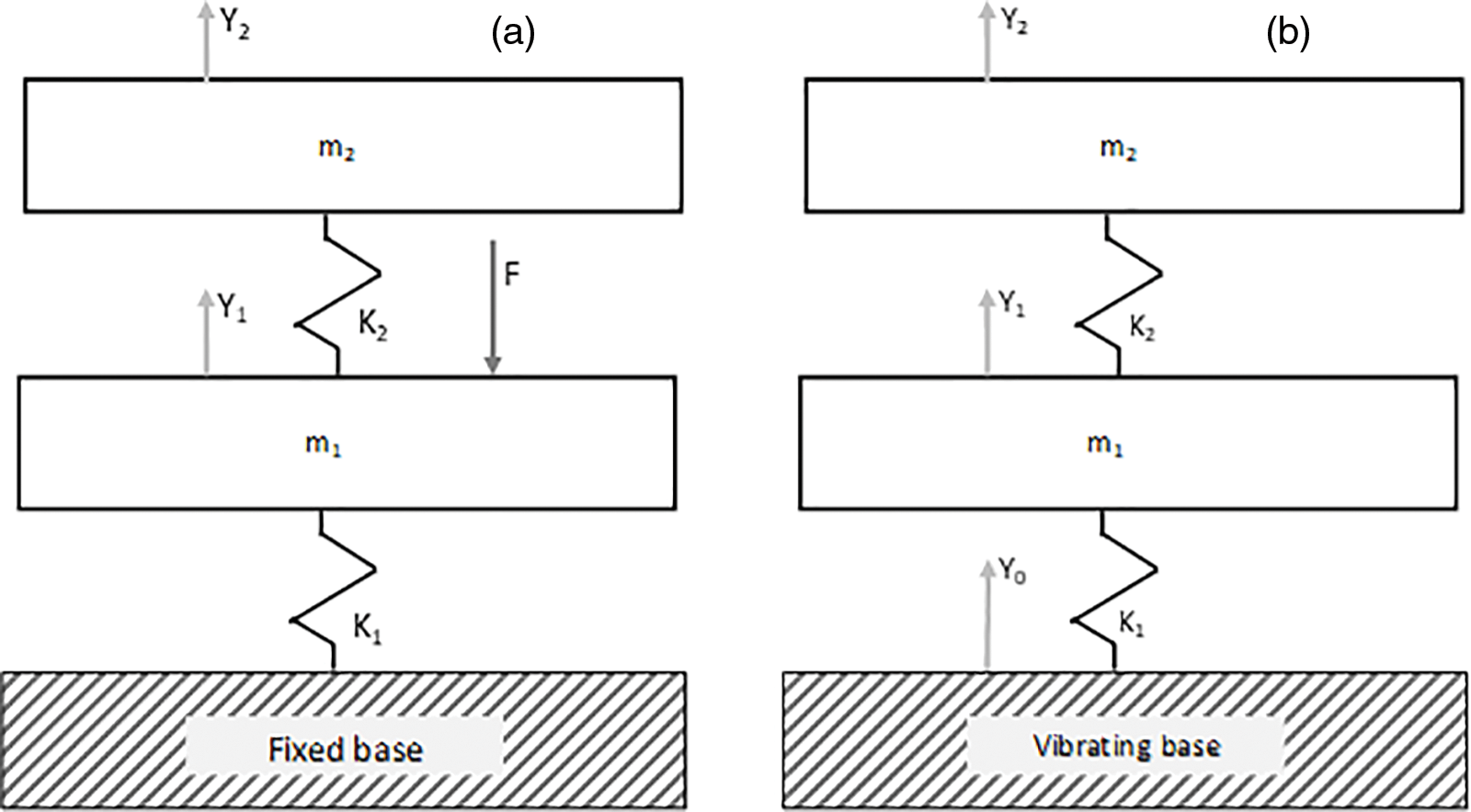
Figure 3: Classic (a) and NVH (b) 2-DOF linear models of mechanical vibration systems

Consider that the rigid base vibrates with the displacement Y0=y0eiωt ; the masses of the first and second rigid elements are m1 and m2 ; both damping and elastic properties are combined in the springs via the complex stiffnesses K1=k1(1+iηp1) and K2=k2(1+iηp2) . Here, k1 and k2 are the real stiffnesses; ηp1 and ηp2 are the partial loss factors (all the parameters are constant values).

The imaginary parts of the complex stiffnesses are positive because of the plus-sign oscillating factor eiωt (see Chapter 3.4). The equations of motion can be written as

{ mY¨1​​​​+K1Y1+K2(Y1−Y2)=K1y0eiωt,                  mY¨2​​​​+K2(Y2−Y1)=0 . (15)

Here Y1=y1eiωt and Y2=y2eiωt are the displacements of the first and second mass, respectively.

4.2 Characteristic Equation and Its Roots

The characteristic equation for Eq. (15) is a quadratic equation with the unknown value Ω2 :

Ω4−Ω2[ωp12(1+iηp1)+ ωp22(1+iηp2)(1+μ)]+ ωp12ωp22(1+iηp1)(1+iηp2)=0  (16)

where the mass ratio

μ= m2/m1 (17)

and

p= ωp2/ωp1 (18)

The ratio of the partial undamped natural angular frequencies is ωp1=k1/m1 and ωp2=k2/m2 .

The roots of Eq. (16) are

Ω~2,12= Ω2,12(1+iηp1,2) (19)

where Ω1 and Ω2 are the undamped natural angular frequencies ( Ω2> Ω1 ), and η1 and η2 are the relevant loss factors of the 2-DOF system. As shown in papers [11,12], upon neglecting the very small values η1η2 and ηp1ηp2 , one can obtain

Ω2,1=ωp1(1+b)(1±1−r  )/2, (20)

η1,2=η±(b−1)2(b+1)1−r(ηp1−ηp2) (21)

where the average loss factor

η=ηp1+ηp22, (22)

r=11+μ4b(1+b)2, (23)

b=p2(1+μ). (24)

From Eqs (23), (20), four interesting conditions can be derived

(1) η1+η2=ηp2+ηp2, 

(2) η1→ηp1 and η2→ηp1 if the parameter b≫1 ,

(3) η2→ηp1 and η1→ηp1 if the parameter b≪1 ,

(4) η1=η2=η  if the parameter b=1 .

The first condition may be related to the Energy Conservation Law. The other three conditions indicate that both loss factors of the 2-DOF in-series system may notably depend on the dimensionless parameter b. Here, the condition b=1 is most important because in this case the loss factors of the 2-DOF system get similar even if the partial loss factors are different.

4.3 The Nearby Natural Frequency Case

As follows from Eqs. (24) and (18), the condition b=1 is equivalent to

p=ωp2ωp1=11+μ. (25)

In this case, parameter r , given by Eq. (23), attains its maximum

rmax=11+μ ,  (26)

The undamped natural frequencies of the 2-DOF system are defined by equation

Ω2,1=ωp11±1−rmax  , (27)

And the ratio of the undamped natural frequencies q=Ω1/Ω2 attains its minimum

qmin=1+μ − μ  (28)

For the given mass ratio μ defined by Eq. (17).

The “tuning formula” (25) describes the nearby natural frequency case where the undamped natural frequencies of 2-DOF in-series system with hysteretic friction and given mass ratio are most close to each other. In this case, as shown above, the loss factors of the 2-DOF system are similar and equal to the average loss factor η  given by Eq. (22).

4.4 Transmissibility Functions in the Nearby Natural Frequency Case

Using Eq. (15), calculate the ratio of the displacement amplitudes y1 and y2 of the first and second masses to the base displacement amplitude y0 :

y1y0=(1+iηp1)[1−(ω/ωp2)2+iηp2]Ψ(ω) , (29)

y2y0=(1+iηp1)[1+iηp2]Ψ(ω)  (30)

where the polynomial

Ψ(ω)=[1−(ω/Ω1)2+iη1][1−(ω/Ω2)2+iη2]. (31)

It can be noted that Eqs. (29) and (30) are also valid in case if the base does not move (Fig. 3a) and the vibration is excited by harmonic force F=F0eiωt where F0=K1y0 .

Using Eqs. (29)–(31), calculate the transmissibility functions for the main 1-DOF subsystem

T1(ω)=|y1y0|=(1+ηp12)H(ω)Φ(ω) (32)

And for the whole 2-DOF system

T2(ω)=|y2y0|=(1+ηp12)(1+ηp22)Φ(ω) (33)

where the functions H(ω) and Φ(ω) are given by equations

{H(ω)=[1−(ω/ωp2)2]2+ηp22 ,Φ(ω)={[1−(ω/Ω1)2]2+η12} {[1−(ω/Ω2)2]2+η22}. (34)

To illustrate the most important physical effects, several transmissibility functions for the main and auxiliary subsystems are calculated using Eqs. (32) and (33) and plotted in Figs. 4 and 5.

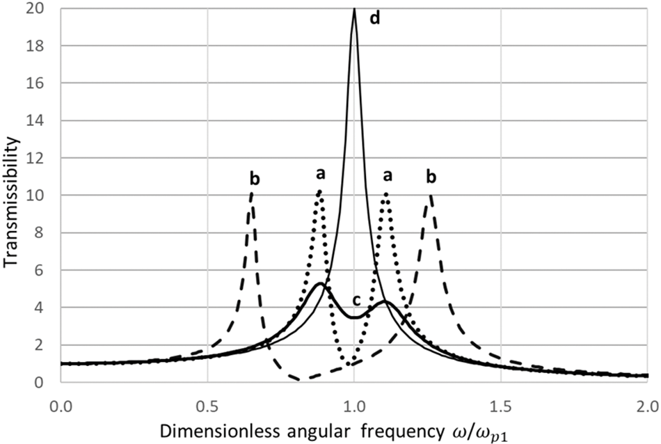
Figure 4: Transmissibility in the nearby natural frequency case for the main subsystem of 2-DOF in-series system if (a) μ=0.05, ηp1=ηp2=0.05; (b) μ=0.5, ηp1=ηp2=0.05; (c) μ=0.05, ηp1=ηp2=0.25; (d) for comparison with the 1-DOF system: μ=0, ηp1=0.05 (no auxiliary system)

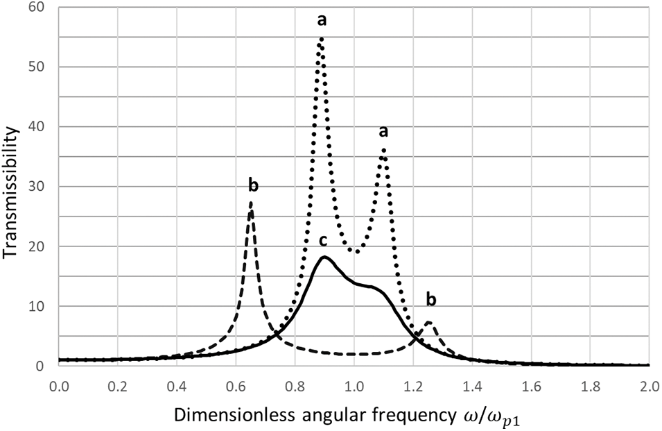
Figure 5: Transmissibility in the nearby natural frequency case for the auxiliary subsystem of 2-DOF in-series system if (a) μ=0.05, ηp1=ηp2=0.05; (b) μ=0.5, ηp1=ηp2=0.05; (c) μ=0.05, ηp1=ηp2=0.25

As seen in Fig. 4, the vibration of the main subsystem is notably lower than that for the 1-DOF system (without the auxiliary subsystem) and this difference grows with the partial loss factor of the auxiliary subsystem. On the other hand, as seen in Fig. 5, the vibration of the auxiliary subsystem may be very high. Thus, in the nearby natural frequency case, the 2-DOF in-series system with hysteretic friction works as a tuned mass damper [4,10–12] with the “tuning formula” given by Eq. (25). More simple and useful analytical relationships can be found in paper [11].

The theory of such a tuned mass damper was originally developed for 2-DOF systems with viscous friction [2–4]. The physical effects are about similar to those in case of hysteretic friction but the “tuning formula” is different from Eq. (25) and is given by

p=ωp2ωp1=11+μ (35)

in the classical case of viscous friction.

4.5 Critical Loss Factor

The other important phenomenon is related to the resonance (damped natural) frequencies. In the nearby natural frequency case, the lower resonance frequency relatively does not change much with the average loss factor. On the other hand, the upper resonance frequency can reduce notably. As a result, the higher-frequency resonance peak fully vanishes in the vibration spectrum of the auxiliary subsystem (Fig. 5). Such a degenerate case happens [13] if the average loss factor equals or exceed its critical value.

ηcr≈0.354 (1−q2) (36)

where q=Ω1/Ω2 is the ratio of the undamped natural frequencies of the 2-DOF system.

5  Internal, Structural, and Total Loss Factors for Diffuse Vibration Fields in thin Plates

The ideal model of diffuse sound field for air volumes is widely applied to calculate the sound energy distribution and propagation in rooms and other enclosures. It suggests that the acoustic energy is uniform (the same everywhere inside a room) and isotropic (the flow of acoustic energy in all directions is equally probable). The diffuse-field model is reasonably valid at relatively high frequencies and is formed by multiple reflections of the free sound or vibration waves from the boundaries (for example, room walls or rod edges).

Here, one of the most important parameters is the mean-free path which is the average distance travelled by sound or vibration waves between successive reflections from the boundaries. In particular, the mean-free path for the diffuse vibration field in a thin rod is the length of the rod. It is true for both longitudinal and bending waves. For a thin plate, the mean-free path is given by

L=πS/P (37)

where S and P are respectively the area and perimeter of the plate (for comparison, the mean-free path for the diffuse sound field in a room is L=4V/S where V and S are the room volume and area). The other important parameter is the average boundary sound (vibration) absorption coefficient α which is defined as the ratio of the energy, absorbed on the boundary, to the incident sound (vibration) wave energy. Both mean-free path and boundary absorption coefficient are averaged over a large number of reflections and directions of wave propagation inside the field region.

Let us estimate the loss factor for the diffuse harmonic vibration field with the mean-free path L , average vibration absorption α , and angular frequency ω . For simplicity, the internal vibration absorption (in the material between the boundaries) is first neglected.

The average time between successive reflections is τ=L/C where C is the free vibration wave speed. Hence, the corresponding number of cycles calculates n=fτ=fL/C where f is the vibration frequency. Therefore, the average vibration energy dissipated per cycle because of the boundary absorption equals D=αℰ/n=(αℰC)/(fL) where ℰ is the average vibration energy. Substituting this value into Eq. (1), calculate the so-called structural loss factor

ηstr=αCωL. (38)

For a thin plate, the speed of free bending waves can be given by equation C=C0f/f0 where C0 and f0 are respectively the sound speed in air and critical coincidence frequency of the plate for airborne sound transmission. In this important case, Eq. (38) can be rewritten in the form

ηstr= αC02πff0 L     (39)

where parameter L is given by Eq. (37).

The total loss factor of bending vibration of a thin plate is

ηtot= ηint+ηstr  (40)

where ηint is the internal loss factor which characterizes the internal absorption in the region between the boundaries [14,15].

Both internal and structural loss factor is high for triplexes, laminated glass panes consisting of two glass panes coupled with a transparent polyvinylbutyral film (commonly 0.7 or 1.4 mm thick [16]). The thickness and coincidence frequency of a laminated pane are about identical to those of a common glass pane of the same surface density. For instance, a triplex made of two 4 mm “ordinary” panes coupled with a polyvinylbutyral film 1.44 mm thick has a surface density of 24 kg/m2 and coincidence frequency of 1250 Hz (close to the parameters of an “ordinary” glass pane 9.5 mm thick). The frequency characteristics of the sound transmission loss for such panes (1.3 × 0.9 m2) are compared in Fig. 6.

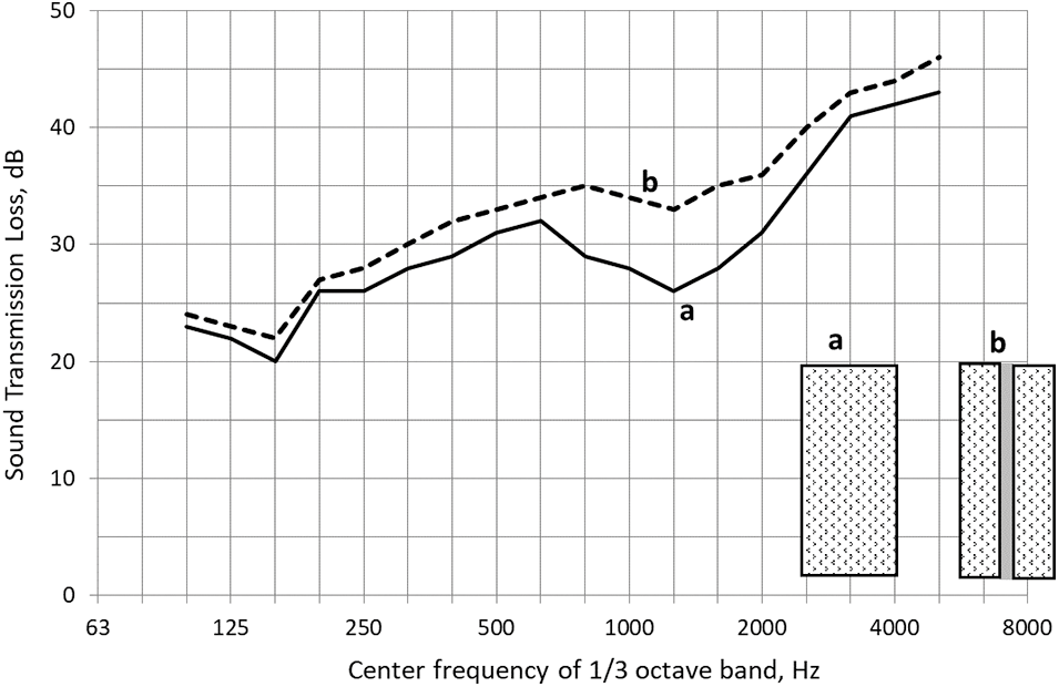
Figure 6: Frequency characteristics of the sound transmission loss for two glass panes of the same mass density and total thickness: (a) ordinary pane, 9.5 mm thick, and (b) triplex (two 4 mm “ordinary” panes coupled with a polyvinylbutyral film 1.44 mm thick)

As seen, the sound transmission loss of triplex is higher: in particular, by 5–7 dB at 800–2000 Hz (in the range centered at the coincidence frequency).

6  Conclusions

The paper is written as a brief tutorial for engineering students and specialists in the areas of NVH analysis and testing, mechanical and aeromechanical design, and noise and vibration control in buildings. The loss factors and their effect on resonance peaks in various mechanical systems are reviewed for acoustic, vibration, and vibration fatigue applications.

The well-known features (complex module of elasticity, total loss factor, etc.) are clarified, and new results are presented (in particular, for 2-DOF in-series models with hysteresis friction). The classic and NVH models of mechanical systems are considered for analysis.

The results can be of both educational and practical interest in particular because some of the known terms and equations were not clearly explained in the standards and engineering textbooks (for instance, why the complex modulus of elasticity is defined with the positive or negative imaginary part).

Acknowledgement: None.

Funding Statement: The author received no specific funding for this study.

Author Contributions: All by Roman Vinokur.

Availability of Data and Materials: None.

Conflicts of Interest: The author declares that he has no conflicts of interest to report regarding the present study.

References

1. ASA 6-1976 (ANSI S2.9-1976) (2006). Nomenclature for specifying damping properties of materials. New York: Acoustical Society of America. [Google Scholar]

2. Harris, C. M., Crede, C. E. (1976). Shock and vibration book, vol. 2. New York: McGraw-Hill Book Company. [Google Scholar]

3. Measurement of the complex modulus of elasticity: A brief survey. Brüel & Kjær Application Notes. https://www.bksv.com/media/doc/BO0061.pdf [Google Scholar]

4. Den Hartog, J. P. (1985). Mechanical vibrations. New York: Dover Publications, Inc. [Google Scholar]

5. Morse, P. M. (1981). Vibration and sound. New York: Acoustical Society of America. [Google Scholar]

6. Timoshenko, S., Young, D. H., WeaverJr, W. (1979). Vibration problems in engineering, 4th editionNew York: John Wiley & Sons. [Google Scholar]

7. Vinokur, R. (2013). Correct sign for imaginary part in the complex modulus of elasticity. INTER-NOISE and NOISE-CON Congress and Conference Proceedings, Internoise 2013, Innsbruck, Austria. [Google Scholar]

8. Vinokur, R. (2003). The relationship between the resonant and natural frequency for non-viscous systems. Journal of Sound and Vibration, 267, 187–189. [Google Scholar]

9. Vinokur, R. (2003). Feasible analytical solutions for electrostatic parallel-plate actuator or sensor. Journal of Vibration and Control, 10(3), 359–369. [Google Scholar]

10. Vinokur, R. (2017). The closed-form theory of tuned mass damper with hysteretic friction. https://vixra.org/pdf/1712.0484v1.pdf [Google Scholar]

11. Nashif, A. D., Jones, D. I., Henderson, J. P. (1985). Vibration damping. New York: John Wiley & Sons. [Google Scholar]

12. Sun, C. T., Lu, Y. P. (1995). Vibration damping of structural elements. USA: Prentice Hall PTR. [Google Scholar]

13. Vinokur, R. (2017). Critical loss factor in 2-Dof in-series system with hysteretic friction and its use for vibration control. Preprint at viXra:1612.0033. https://vixra.org/abs/1612.0033 [Google Scholar]

14. Vinokur, R. (1981). Influence of the edge conditions on the sound insulation of a thin finite panel. Soviet Physics–Acoustics, 26(1), 72–73. [Google Scholar]

15. Craik, R. (1981). Damping of building structures. Applied Acoustics, 14(5), 347–359. [Google Scholar]

16. Vinokur, R. (1996). Evaluating sound-transmission effects in multi-layer partitions. Sound and Vibration, 22–28. [Google Scholar]