
 Submit a Paper
 Propose a Special lssue
 Open Access
ARTICLE

Stochastic Analysis for the Dynamics of a Poliovirus Epidemic Model
1
Department of Mathematics, Government Maulana Zafar Ali Khan Graduate College Wazirabad, Punjab Higher Education
Department (PHED), Lahore, 54000, Pakistan
2
Department of Mathematics, Cankaya University, Balgat, Ankara, 06530, Turkey
3
Department of Medical Research, China Medical University, Taichung, 40402, Taiwan
4
Institute of Space Sciences, Magurele-Bucharest, 077125, Romania
5
Department of Dermatology, Rashid Latif Medical College Lahore, Lahore, 54000, Pakistan
6
Department of Mathematics, Technische Universitat Chemnitz, Chemnitz, 6209111, Germany
7
Department of Mathematics and Statistics, The University of Lahore, Lahore, 54590, Pakistan
8
Department of Mathematics, Faculty of Science and Technology, University of Central Punjab, Lahore, 54000, Pakistan
9
Department of Biochemistry, University of Sialkot, Sialkot, 51311, Pakistan
* Corresponding Author: Muhammad Mohsin. Email:
(This article belongs to the Special Issue: Bio-inspired Computer Modelling: Theories and Applications in Engineering and Sciences)
Computer Modeling in Engineering & Sciences 2023, 136(1), 257-275. https://doi.org/10.32604/cmes.2023.023231
Received 15 April 2022; Accepted 30 August 2022; Issue published 05 January 2023
 View Full Text
 Download PDF
Abstract
Most developing countries such as Afghanistan, Pakistan, India, Bangladesh, and many more are still fighting against poliovirus. According to the World Health Organization, approximately eighteen million people have been infected with poliovirus in the last two decades. In Asia, still, some countries are suffering from the virus. The stochastic behavior of the poliovirus through the transition probabilities and non-parametric perturbation with fundamental properties are studied. Some basic properties of the deterministic model are studied, equilibria, local stability around the stead states, and reproduction number. Euler Maruyama, stochastic Euler, and stochastic Runge-Kutta study the behavior of complex stochastic differential equations. The main target of this study is to develop a nonstandard computational method that restores dynamical features like positivity, boundedness, and dynamical consistency. Unfortunately, the existing methods failed to fix the actual behavior of the disease. The comparison of the proposed approach with existing methods is investigated.Keywords
Jenkins et al. in 2006 formulated a model in which he concluded that the use of monovalent is better than other vaccines. It provides outstanding outbreak control [1]. Haldar et al. [2] introduced the poliovirus vaccine in India. Kalkowska et al. in 2020 represent a differential equation-based stochastic model for poliovirus transmission. The model shows the poliovirus transmission for 2019 to 2023 with a strategic eradication plan [3]. Minor studied the types of polioviruses, vaccination, and eradication of the virus worldwide [4]. Thompson [5] investigated the transmission dynamics of the poliovirus in Nigeria. Duque-Marin et al. [6] studied two types of vaccines in the mathematical model. Denes et al. [7] presented a model which describes polio transmission in tropical regions. Cheng et al. [8] discussed a polio vaccination model in two different age classes. Alba et al. [9] addressed the correlation between climate and vaccination through a mathematical model. Shaghaghi et al. in 2018, studied that the OPV and IVPPvs vaccine was helpful for the eradication of the virus last few years [10]. Shimizu in 2014 [11] explained IPV is very effective against the poliovirus, and the author reviewed the introduction, development, and characterization of the OPV vaccine. In addition, his place in the world was told. Rafique et al. in 2020 presented a mathematical model in which they discovered the dynamics of poliovirus transmission using standard methods with vaccination [12]. Nidia et al. [13] in 2007, examined the effects of the poliovirus on human life and the steps taken to eradicate the virus and discussed what steps we could take in the future to get rid of it. Thompson et al. [14] presented polio outbreaks in the USA. Kalkowska et al. introduced a model to identify poliovirus and opportunities to increase population immunity [15]. Kim et al. [16] presented a model to examine the transmission of virulent circulating vaccine-derived polioviruses. Hillis [17] formulated a model in different regions before using artificial poliovirus vaccination. Mendrazitsky et al. [18] explained a disease of epidemic development model. The model analyzed other properties of polio and its non-equilibrium outbreak dynamics. Debanne et al. [19] presented a mathematical model of poliovirus in America. Naik et al. [20,21] studied the fractional modeling of cancer and HIV infection with the well-known results of stabilities.
The strategy of the paper is as follows. The first section goes to literature, and Section 2 goes to stochastic modeling of poliovirus and its fundamental properties. Section 3 goes to the proposed numerical method and its simulation with current approaches in the literature. Section 4 goes to the paper’s conclusion and remarks.
For any time
with initial condition S (0) ≥ 0; E (0) ≥ 0; I (0) ≥ 0; V (0) ≥ 0, and
2.1 Properties [24]
This section studies the positivity and boundedness of the system ((1)–(4)). Let us consider the vector as follows:
And the norm
As,
If L acts on a function
where transportation is denoted by
Theorem 1: For model ((1)–(4)) and any given initial value
Proof: By Ito’s formula, the model ((1)–(4)) admits a positive solution in the unique local on
Next, let us show that the given model ((1)–(4)) admits this solution in the global sense; that is,
Let
where we set
Then
In case of violation of statement, then
this, there is an integer
Define a
By using Ito’s formula, we calculate
Let,
By integrating from 0 to
where
Set
Hence,
Then we obtain
As desired.
The disease-free equilibrium of the model is
The endemic equilibrium of the model is denoted by K1 = (S*, E*, I*, V*).
Theorem 2: The disease-free equilibrium
Proof: Considering the function from the system ((1)–(4)) as follows:
The elements of the given Jacobean Matrix at
We obtain the following results by applying Routh Hurwitz criteria for 2nd order.
Theorem 3: The endemic equilibrium K1 = (S*, E*, I*, V*) is locally asymptotically stable if
Proof: The Jacobean matrix at
where
Applying Routh-Hurwitz Criterion for 3rd order,
Hence the given system is locally asymptotically stable.
The idea of reproduction number is presented in [25] by considering Eqs. (3) and (4), we get the following matrices:
Here, F =
The spectral radius of the
where
3 Stochastic Poliovirus Epidemic Model
Let us consider the vector
The equation of poliovirus epidemic model ((1)–(4)) can be written as
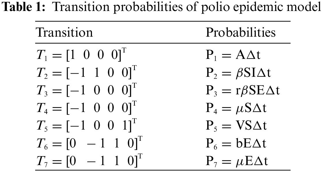
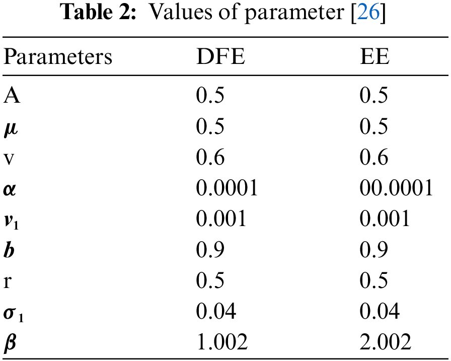
The Euler Maruyama approach is cast-off to determine the numerical result of the Eq. (17) by using the values of the parameters given in Table 2 as follows:
where
3.1 Stochastic Nonstandard Finite Difference Method
The stochastic NSFD can be developed for the system ((1)–(4)) as
The breakdown of the proposed method for the above equation.
Similarly, we break the remaining system into a proposed method like (19), as follows:
where, n = 0, 1, 2,…, and discretization gap is denoted by “h”.
Theorem 5: The stochastic NSFD method is stable if the eigenvalues of Eqs. (19)–(22) lie in the unit circle for any
Proof: Let the functions L1, L2, L3, L4 by assuming
The elements of the Jacobean matrix are given as
The given Jacobean matrix at
Hence, by using the Mathematica software all the eigen values of the above Jacobean matrix lie in the unit circle if
Now, for endemic equilibrium (EE) K1 = (S*, E*, I*, V*). The given Jacobean matrix is
Using Mathematica software, the most many eigenvalues of the Jacobean is less than one when
Fig. 1 admits the comparative analyses of the proposed approach with current methods in the sense of stochastic. The numerical experimentations can easily conclude that other stochastic numerical methods are conditionally convergent or diverge with larger time step values. The nature of biological properties is not consistent with existing literature methods. For this sake, the nonstandard finite difference is designed to restore the structure of continuous models. Computational methods like stochastic Euler, stochastic Runge Kutta, and Euler Maruyama are presented. Unfortunately, these methods are only applicable for the small step size. These methods diverge when we increase the time and do not obey the dynamical properties (positivity, stability, consistency, and boundedness). The stochastic nonstandard finite difference (SNSFD) method is appropriate for all complex and nonlinear stochastic epidemic models. The stochastic model is a reliable and efficient technique to handle highly nonlinear problems close to nature. The stochastic model is the extension of the deterministic model. We present the non-parametric perturbation technique for the said model. Our focus is to propose an always dynamically consistent, positive, and bounded scheme. That is why we investigate the nonstandard finite difference method in the sense of the stochastic. A comparison section is presented for the efficiency of the processes. Furthermore, we extend this idea to other types of models in the future, as shown in [27–31].
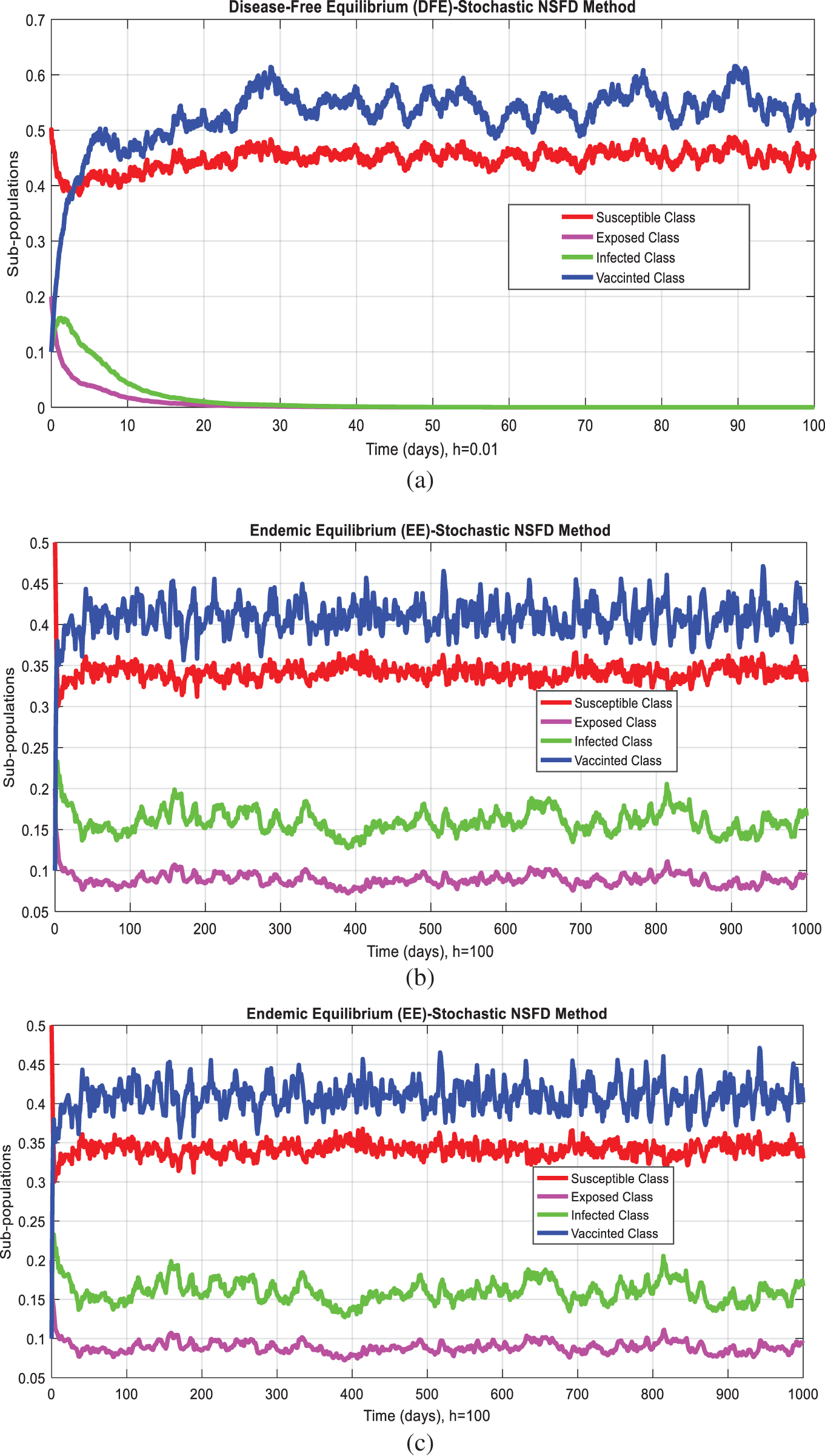
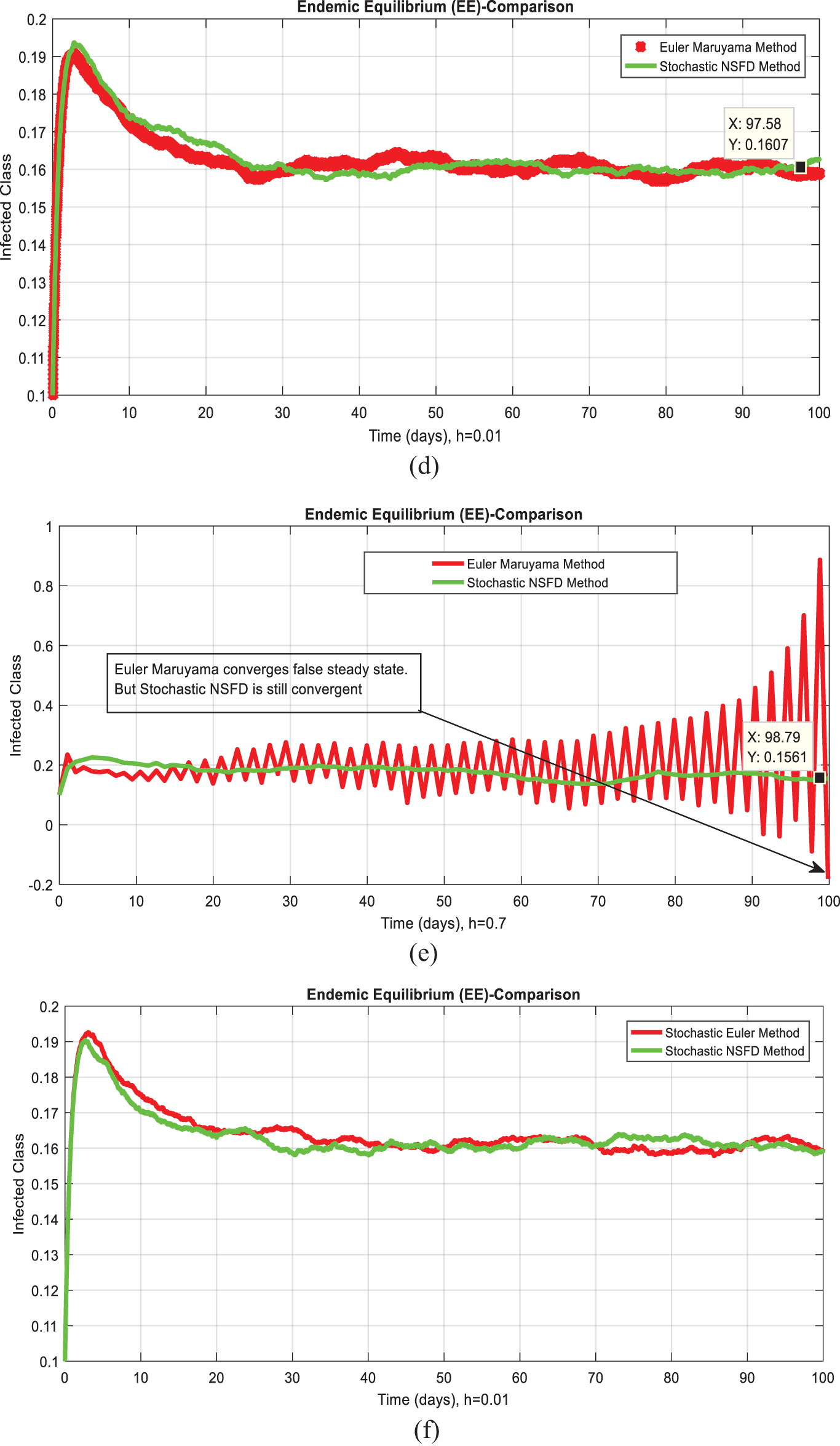
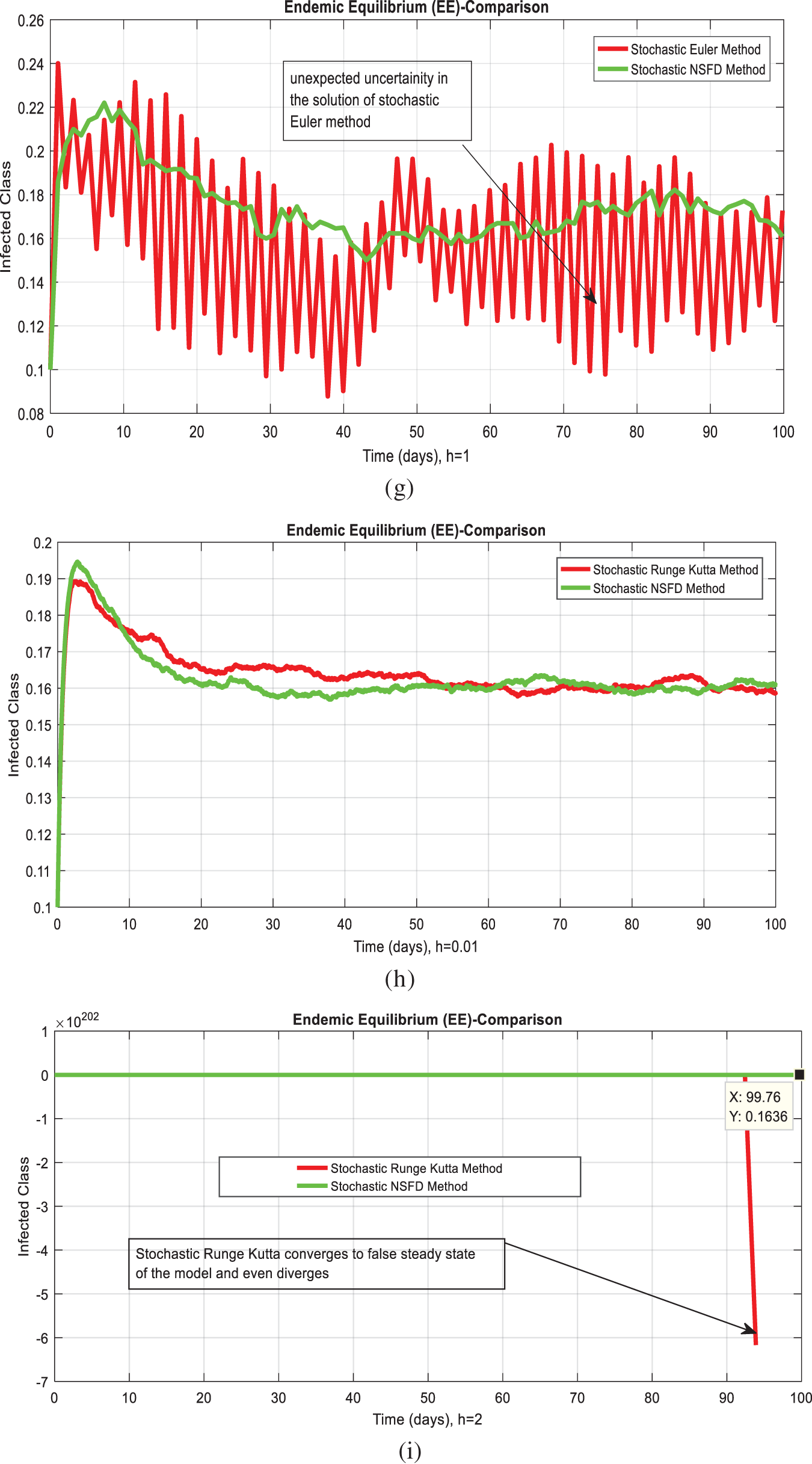
Figure 1: (a) Stochastic NSFD for DFE at h = 0.01 (b) Stochastic NSFD at h = 100 (c) stochastic NSFD for EE at h = 100 (d) Infected class (comparison) at h = 0.01 (e) Infected class (comparison) at h = 0.7 (f) Infected class (comparison) at h = 0.01 (g) Infected class (comparison) at h = 1 (h) Infected class (comparison-RK) of at h = 0.01 (i) Infected class (comparison-RK) at h = 2
Acknowledgement: Thanks to all authors who contributed equally to preparing the article.
Funding Statement: The authors received no specific funding for this study.
Conflicts of Interest: The authors declare that they have no conflicts of interest to report regarding the present study.
References
1. Jenkins, P. C., Modlin, J. F. (2006). Decision analysis in planning for polio outbreak in the United States. Pediatrics, 118(2), 611–618. DOI 10.1542/peds.2005-2358. [Google Scholar] [CrossRef]
2. Haldar, P., Agrawal, P., Bhatnagar, P., Tandon, R., McGray, S. et al. (2019). Fractional-dose inactivated poliovirus vaccine, India. Bulletin of the World Health Organization, 97(5), 328–334. DOI 10.2471/BLT.18.218370. [Google Scholar] [CrossRef]
3. Kalkowska, D. A., Pallansch, M. A., Wassilak, S. G., Cochi, S. L., Thompson, K. M. (2021). Global transmission of live polioviruses: Updated dynamic modeling of the polio endgame. Risk Analysis, 41(2), 248–265. DOI 10.1111/risa.13447. [Google Scholar] [CrossRef]
4. Minor, P. D. (2016). An introduction to poliovirus: Pathogenesis, vaccination, and the endgame for global eradication. In: Poliovirus, pp. 1–10. New York, NY: Humana Press. [Google Scholar]
5. Thompson, J. E. (2014). A class structured mathematical model for polio virus in Nigeria. https://www.math.tamu.edu/undergraduate/research/REU/results/REU_2014/JaneThompsonPaper.pdf. [Google Scholar]
6. Duque-Marín, E., Vergaño-Salazar, J. G., Duarte-Gandica, I., Vilches, K. (2019). Mathematical modelling of some poliomyelitis vaccination and migration scenarios in Colombia. Journal of Physics: Conference Series, 1160, 012021. DOI 10.1088/1742-6596/1160/1/012021. [Google Scholar] [CrossRef]
7. Denes, A., Szekely, L. (2017). Global dynamics of a mathematical model for the possible re-emergence of polio. Mathematical Biosciences, 293(1), 64–75. DOI 10.1016/j.mbs.2017.08.010. [Google Scholar] [CrossRef]
8. Cheng, E., Gambhirrao, N., Patel, R., Zhowandai, A., Rychtar, J. et al. (2020). A game theoretical analysis of poliomyelitis vaccination. Journal of Theoretical Biology, 499, 110298. DOI 10.1016/j.jtbi.2020.110298. [Google Scholar] [CrossRef]
9. Alba, G. D., Rebolledo, Z. A., Suavez, P. (1976). Influence of climate and vaccination on the incidence of poliomyelitis. Salud Publica de Mexico, 18(1), 509–517. [Google Scholar]
10. Shaghaghi, M., Soleyman-Jahi, S., Abolhassani, H., Yazdani, R., Azizi, G. et al. (2018). New insights into physiopathology of immunodeficiency associated vaccine derived poliovirus infection systematic review of over five decades of data. Vaccine, 36(13), 1711–1719. DOI 10.1016/j.vaccine.2018.02.059. [Google Scholar] [CrossRef]
11. Shimizu, H. (2016). Development and introduction of inactivated poliovirus vaccines derived from sabin strains in Japan. Vaccine, 34(16), 1975–1985. DOI 10.1016/j.vaccine.2014.11.015. [Google Scholar] [CrossRef]
12. Rafique, M., Shahid, N., Ahmed, N., Shaikh, T. S., Asif, M. et al. (2020). Efficient numerical method for the solution of the poliovirus epidemic model with the role of vaccination. Scientific Inquiry and Review, 4(16), 16–30. DOI 10.32350/sir/2020/44/1052. [Google Scholar] [CrossRef]
13. Jesus, N. H. D. (2007). Epidemics to eradication: the modern history of poliomyelitis. Virology Journal, 4, 70. DOI 10.1186/1743-422X-4-70. [Google Scholar] [CrossRef]
14. Thompson, K. M., Wallace, G. S., Tebbens, R. J. D., Smith, P. J., Barskey, A. E. et al. (2012). Trends in the risk of US polio outbreaks and polio virus vaccine availability for response. Public Health Reports, 127(1), 23–37. DOI 10.1177/003335491212700104. [Google Scholar] [CrossRef]
15. Kalkowska, D. A., Tebbens, R. J. D., Thompson, K. M. (2014). Modeling strategies to increase population immunity and prevent poliovirus transmission in two high risk areas in Northern India. Journal of Infectious Disease, 210(1), 398–411. DOI 10.1093/infdis/jit844. [Google Scholar] [CrossRef]
16. Kim, J. H., Rho, S. H. (2015). Transmission dynamics of oral polio vaccine viruses and vaccine derived poliovirus on networks. Journal of Theoretical Biology, 364(1), 266–274. DOI 10.1016/j.jtbi.2014.09.026. [Google Scholar] [CrossRef]
17. Hillis, A. (1979). A mathematical model for the epidemiologic study of infectious diseases. International Journal of Epidemiology, 8(1), 167–176. DOI 10.1093/ije/8.2.167. [Google Scholar] [CrossRef]
18. Mendrazitsky, S. B., Stone, L. (2005). Modeling polio as a disease of development. Journal of Theoretical Biology, 237(1), 302–315. DOI 10.1016/j.jtbi.2005.04.017. [Google Scholar] [CrossRef]
19. Debanne, S. M., Rowland, D. Y. (1996). Statistical certification of eradication of poliomyelitis in the Americas. Mathematical Bioscience, 150(1), 83–103. DOI 10.1016/S0025-5564(98)00007-8. [Google Scholar] [CrossRef]
20. Naik, P. A., Zu, J., Naik, M. U. D. (2021). Stability analysis of a fractional-order cancer model with chaotic dynamics. International Journal of Biomathematics, 14(6), 1–20. DOI 10.1142/S1793524521500467. [Google Scholar] [CrossRef]
21. Naik, P. A., Zu, J., Owolabi, K. M. (2020). Modeling the mechanics of viral kinetics under immune control during primary infection of HIV-1 with treatment in fractional order. Physica A: Statistical Mechanics and its Applications, 545, 123816. DOI 10.1016/j.physa.2019.123816. [Google Scholar] [CrossRef]
22. Khan, T., Zaman, G., El-Khatib, Y. (2021). Modeling the dynamics of novel coronavirus (COVID-19) via stochastic epidemic model. Results in Physics, 24, 104004. DOI 10.1016/j.rinp.2021.104004. [Google Scholar] [CrossRef]
23. El-Khatib, Y., Al-Mdallal, Q. (2022). On Solving SDEs with linear coefficients and application to stochastic epidemic models. Advances in the Theory of Nonlinear Analysis and its Application, 6(2), 280–286. DOI 10.31197/atnaa.948300. [Google Scholar] [CrossRef]
24. Sene, N. (2020). Analysis of the stochastic model for predicting the novel coronavirus disease. Advances in Difference Equations, 568. DOI 10.1186/s13662-020-03025-w. [Google Scholar] [CrossRef]
25. Driekmann, O., Heesterbeek, J. A. P., Roberts, M. G. (2009). The construction of next-generation matrices for compartmental epidemic models. Journal of Royal Society and Interface, 7(47), 873–885. DOI 10.1098/rsif.2009.0386. [Google Scholar] [CrossRef]
26. Agarwal, M., Bhadauria, A. S. (2011). Modeling spread of polio with the role of vaccination. Applications of Mathematics, 6(12), 552–571. [Google Scholar]
27. Xu, Y., Wei, L., Jiang, X., Zhu, Z. (2021). Complex dynamics of a SIRS epidemic model with the influence of hospital bed number. Discrete & Continuous Dynamical Systems–B, 26(12), 6229–6252. DOI 10.3934/dcdsb.2021016. [Google Scholar] [CrossRef]
28. Lu, C. (2022). Dynamical analysis and numerical simulations on a crowley-martin predator-prey model in stochastic environment. Applied Mathematics and Computation, 413, 126641. DOI 10.1016/j.amc.2021.126641. [Google Scholar] [CrossRef]
29. Haokun, Q., Meng, X. (2021). Mathematical modeling, analysis and numerical simulation of HIV: The influence of stochastic environmental fluctuations on dynamics. Mathematics and Computers in Simulation, 187(1), 700–719. DOI 10.1016/j.matcom.2021.03.027. [Google Scholar] [CrossRef]
30. Shatanawi, W., Raza, A., Arif, M. S., Rafiq, M., Bibi, M. et al. (2021). Essential features preserving dynamics of stochastic dengue model. Computer Modeling in Engineering & Sciences, 126(1), 201–215. DOI 10.32604/cmes.2021.012111. [Google Scholar] [CrossRef]
31. Arif, M. S., Raza, A., Abodayeh, K., Rafiq, M., Bibi, M. et al. (2020). A numerical efficient technique for the solution of susceptible infected recovered epidemic model. Computer Modeling in Engineering & Sciences, 124(2), 477–491. DOI 10.32604/cmes.2020.011121. [Google Scholar] [CrossRef]
Cite This Article
 Copyright © 2023 The Author(s). Published by Tech Science Press.
This work is licensed under a Creative Commons Attribution 4.0 International License , which permits unrestricted use, distribution, and reproduction in any medium, provided the original work is properly cited.
 Downloads
 Citation Tools