Automated Classification of Snow-Covered Solar Panel Surfaces Based on Deep Learning Approaches

1  Introduction

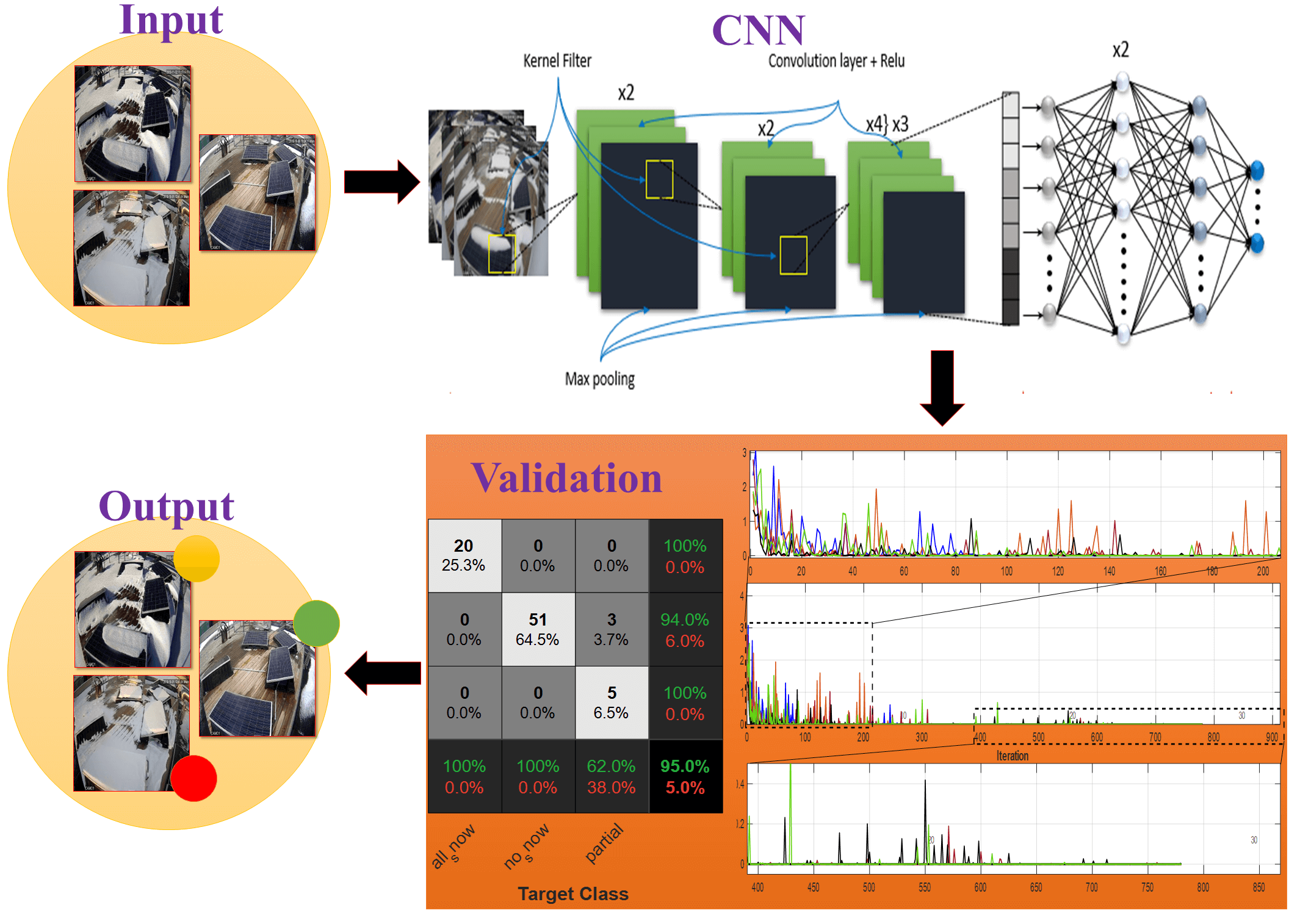
In the last few years, artificial intelligence (AI), especially deep learning (DL), has become the mainstay in many studies, such as image classification and recognition. Image classification and recognition are the subjects of many applications in different fields [1]. It constitutes a large domain, and there are still many unexplored arguments [2]. Deep learning enables the extraction of significant features from the fed feature spaces and obtaining higher classification potential. The convolutional neural network models are used to extract features and classify images based on the obtained output in the last layer (fully connected) where the final decision is made. The main purpose of feature extraction in images is to reduce the amount of redundant large data and extract informative features that improve and speed up the image and classification process. In some image datasets, such as medical X-ray images, thermal images, animal images of the same breed, etc., there are very high similarities in the features between classes that made the models suffer from distinguishing between them; therefore, robust models need to be used.

Deep learning techniques have been specifically developed to deal with the classification of image data. The main challenge is increasing the capabilities of deep learning techniques to distinguish and classify highly similar images. Convolutional neural networks (CNN) have many models, namely; VGG16, VGG19 [3], and ɌESNET-18, ɌESNET-50, and ɌESNET-101 [4], which we will use in this research paper.

Various models have been used to solve many problems related to these issues. Ahsan et al. [5] used six different models of convolutional neural networks to detect COVID-19 using X-ray images. In their paper, they used two different types of datasets; one balanced and the other unbalanced. The results show that the two models VGG16 and MobileNetV2 outperform the rest of the models according to the recognition accuracy, where the x-rays indicate whether the patient has COVID-19 or not. In [6–8], authors used ResNet model with segmentation on the computed tomography (CT) dataset of Covid patients. The results verified the performance behavior by giving high accuracy. Ishengoma et al. [9], relied on the image dataset they obtained through UAV to detect the maize leaves were infected by fall armyworms (faw) in their study. The study was conducted on deep learning models, namely; VGG16, Vgg19, InceptionV3, and MobileNetV2. Furthermore, the researchers added an image improved model by applying Shi-Tomas. The results showed that these models have high accuracy in detecting infected leaves. On the other hand, the image optimization process used for the images has significantly and positively increased the efficiency of the models used. Zhu et al. [10] studied the quality of the appearance of the islands based on 12 models of deep learning, where the researchers added a Support vector machine (SVM) to the proposed models and the study demonstrated accuracy. The results showed that the addition of SVM significantly increased the accuracy of the model.

Regarding some related works, several studies have been conducted on snow loss. Researchers presented methods for predicting daily snow losses based on intelligent techniques that can help to reduce operational risks [11].

The reliance on solar energy has increased significantly recently [12], as solar energy constituted the most reliant percentage of renewable energies. Solar panels are the only way to convert solar energy into electrical energy. These panels are affected by the climate. As it is known in winter season, low temperatures and snowfall have negative impact on these panels. Snow prevents sunlight photons from reaching the surface of the solar panels; thus, electricity production is reduced at the level of the solar panel system used in the place of snowfall. The overall electricity production losses from solar panels in winter are more than 25% [13], and can be more than 90% if the panels are completely covered with snow [14]. In regions that receive a significant amount of snowfall annually, such as Germany, Canada, Turkey, UK and USA, system performance is impacted; consequently, the output power is reduced. As a result of the snow that has accumulated on the panels [15,16].

Several studies have been conducted to improve the performance of solar power systems and use modern systems to benefit from the largest amount of solar energy [17–20]. The state estimation and prediction for the photovoltaic system are critical as it is very important in avoiding losses due to external influences on the system. In [21], a new method for calculating the efficiency of the solar panel system in case of snowy weather and low levels of insolation was proposed; the study also clarified that using the Bouguer-Lambert Law, the insolation level of a snow-covered solar panel surface can be estimated. In [22], the authors presented a state estimation study of two types of solar panels (monofacial and bifacial) for severe winter climate. The study calculated the snow losses in winter for the two types of models. The results have shown that the snow losses for monofacial and bifacial are within average (33% and 16%, respectively) for the winter season and (16% and 2%, respectively) on an annual rate. It is necessary to remove snow from the solar panels to take advantage of the largest amount of solar energy and reduce snow losses. Before starting the snow removal process, snow-covered panels should be effectively distinguished. This can improve snow removal speed and removal efficiency. This paper aims to classify solar panels based on the similarity in images, including; size, color, and general appearance for images based on convolutional neural network models. The contributions in this paper can be summarized as follows:

(1) We present an efficient framework for solar panel classification using features extraction and a softmax classifier. These two processes are the mainstay of CNN. The five CNN models presented in this work are (VGG-16, VGG-19, ɌESNET-18, ɌESNET-50, and ɌESNET-101). The strengths and weaknesses of each model have been well investigated, as well as the classification accuracy of the models considering three splits; training, validation, and testing dataset.

(2) The dataset used in this work consists of three categories, namely, no_snow, partial snow, and all_snow. These categories represent the normal state of solar panels under steady-state conditions. The first case was conducted with data without any kind of preprocessing, as it used clear images and an unbalanced dataset. Also, some data samples from the partial class covered with a very small snow zone (approximately 5%) are moved to the no snow class in order to make the classification more complicated.

(3) Unsteady-state environmental conditions occur in the work environment, making it necessary for us to simulate these conditions and evaluate the models in these complex conditions. Extreme climate conditions will be simulated by generating motion noise. On the other hand, to balance the data, the partial class samples were replicated using the upsampling technique to improve the performance of the experiment. Snow-covered panels from 1% to 99% are classified as partial and 100% as all snow. Finally, the solar panels were classified into three categories, no_snow, partial, and all_snow.

(4) The proposed CNN models in Step (1) and using the dataset in Steps (2) and (3) were applied. Finally, the models are evaluated in both cases, and the results of different metrics are presented.

2  Materials and Methods

2.1 Case Study

In this study, we considered Karabuk University located in Karabuk Province west of the Black Sea region in northern Turkey, as a case study. Karabuk Province is one of the snowiest provinces in winter. Karabuk University is located in the state of Karabuk with Geographical coordinates (41.211242°, 32.656032°) [23]. In the Karabuk region, summers are warm and clear, and winters are very cold, snowy, and partly cloudy. The temperature normally ranges between −1°C and 29°C throughout the year, rarely below −8°C and above 34°C. With a temperature of 20.8°C, August is the hottest month of the year. The average temperature in January is 0.1°C, which is the lowest average of the year, as we see in Fig. 1, Karabuk University will be highlighted as a snowy area that causes losses in photovoltaic energy. Karabuk University is characterized by the presence of a large number of solar panels on its roofs and the sides of buildings. As we can see in Fig. 2, Karabük University makes use of these solar panels in the production of electrical energy.

Figure 1: Temperature distribution at 2 meters for all months

Figure 2: Sample images for Karabuk University solar panels with different side views

2.2 Irradiation Per Square Meter

Winter has a significant impact on these panels, as low temperatures and snowfall lead to the formation of a layer of snow on the surface of the solar panels, as there are sunny days that can be used to produce electrical energy. Whereas the accumulation of snow that covers the surface of the solar panels reduces the energy production of the panels and it is difficult to utilize the energy these days. Recently, several methods have been introduced to remove the snow accumulated on solar panel surfaces; one of the recently proposed techniques is the solar panel heating system for photovoltaic systems. Proposing a new method for detecting snow-covered panels is extremely important, then it contributes to accelerating the snow-melting process, where detection is handled and then instructs the heating system to carry out the snow melting process or any other snow removal process.

The study presents a new methodology based on the historical climatic dataset (2021) that can be found on the NASA research website [24]. Figs. 3a and 3b show Direct Normal Irradiation (DNI), which is represented by the amount of radiation falling on the surface in an orthogonal manner without calculating the amount of radiation reflected from cloud particles or others, DNI carries the energy that solar panels use to produce electricity. Fig. 3a shows the sum of the average amount of energy in units of Wh/m² for all months over a 24-h period. The months represented in white color have lower temperatures and snowfall, while the months represented in black color have moderate temperatures and no snowfall; on the other hand, the months represented in orange color mean that the number of sunshine hours is long, which indicates most solar energy falls on the surface. Snowfall negatively affects the production of electrical energy from solar panels, as snowfall has two main issues: Firstly, it prevents the radiation carrying energy from contacting the solar panels and thus reduces the amount of energy; secondly, it constitutes a layer of snow on the solar panels causing damage to the solar panels as well as making panels out of service.

Figure 3: (a) The sum of watt hour per meter square for one day, (b) Average monthly kilowatt-hours per square meter

Fig. 3a shows the sum of irradiation energy by Wh/m² for each month over a 24-h period, as shown in the equation below:

Averagehours=∑EN(1)

Fig. 3b calculating the irradiation energy in kWh/m2 for all months as the following:

TotalAveragemonth=(∑Averagehours)×no.monthdays(2)

where E is irradiation energy and N the count of those hours. The Averagehours (Wh/m2) is the E average of the same hour per day throughout the month. While the TotalAveragemonth (kWh/m²) is the total of Wh/m2 per month.

It is very important to determine the snowfall months to estimate and evaluate the state of the photovoltaic system and forecast the percentage of snow losses in order to overcome this challenge and work to solve it using intelligent techniques. Obviously, Figs. 2 and 3 show the decrease in the irradiation energy during the first three months and the last two months, which is attributed to a lower temperature and snowfall. Snow losses in these five months are high due to the formation of an insulating layer on the solar panels; the percentage of energy losses is estimated by the time the insulation layer remains on the solar panels. Table 1 shows the specific photovoltaic power output (SPPO) values for the five months based on irradiation energy in relation to the number of sunshine hours.

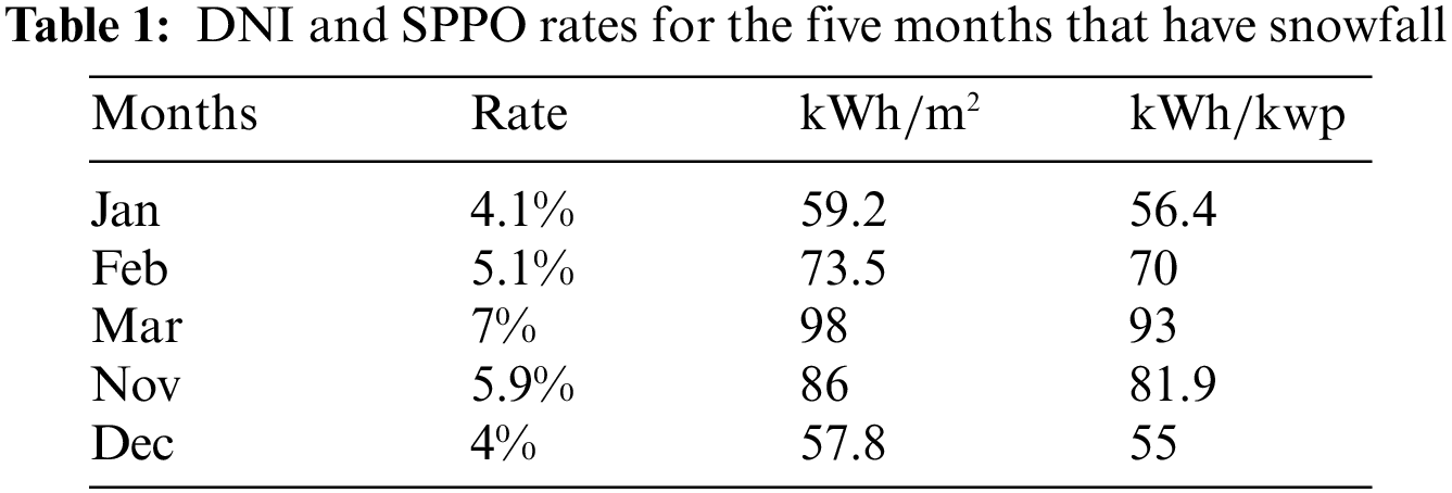
According to our conducted study, the snowfall days in January are nine days then the panels need five additional days to melt the remaining snow on the panels. Therefore, the panels will be 14 days covered by snow. It concludes that the energy produced by the panels during these days is 0%. It has become necessary to find more efficient substitutions using advanced and intelligent technologies that can overcome the obstacles and difficulties facing photovoltaic energy systems, which can contribute to reducing snow losses as well as improving the level of energy production. This research contributes to the advancement of an advance by directing artificial intelligence techniques to solve the problems of energy systems.

2.3 Dataset

In this experiment, the conducted datasets were examined in two different cases; in the first case, the dataset was conducted on the original size with 395 solar panel images in its original size, then the dataset was preprocessed by applying upsampling on the minority sampled classes to be 437 images. This dataset is divided into three categories: all_snow, which represents the images of the panels completely covered by snow; the next category, no_snow, which presents the images of the snow-free panels; and the last category is partial, presents the partial condensation of snow on the panels. Before the data training process, there some preprocessing is performed on the input feature space by resizing the images to 224 × 224 for a regular training process, and then the reconstructed images are fed into the training process. The dataset is divided into 60% training, 20% validation, and 20% testing. Fig. 4 illustrates samples of the conducted dataset in this paper.

Figure 4: Representative samples of solar panels dataset, (a) All snow, (b) No snow, and (c) Partial

2.4 The Models and Features Extraction

The CNN architecture includes three basic layers through which important features are extracted, and the classification process is carried out: convolution layers, pooling layers, and fully connected layers [25–27]. The convolution layer is a major component of the CNN structure, and it is an input receiving layer applying two different operations, kernel or filter and Relu Function. By applying these two currencies, the feature map can be extracted. The pooling layer is usually an appendage with a convolution layer, the purpose of adding a pooling layer is to extract the most important features, thereby reducing data size as well as accelerating the learning process; there are two types of pooling layers are the most common, Average Pooling and Max Pooling. The fully connected layers make the last decision, where the features map is extracted in the previous two layers and converted to a one-dimensional array through Flatten Layer (global average pooling) before entering the fully connected layers.

The output value was calculated for each of the convolution layers as described in the equation below:

Yconv,1,2,3,…=(σ(∑iXi×Wi)+b)(3)

where Yconv,1,2,3,… is the output, σ mean for each kernel scan, X is the input, W is the filter weight matrix, and b is the bias matrix.

Relu function is briefly described as follows:

f(input(x))={ x,x>00,x≤0(4)

The following equation is used to calculate max-pooling layer:

Ymaxpooling =max(Yconv,1,2,3……)(5)

The skip connection of the ResNet model can be defined as

Y=F(X,{Wi})+x(6)

where X is the connection to the layers and x is the skip connection.

Finally, the softmax function is defined as the function that converts a vector of real K values into a vector of real values K whose sum is 1. There are three possible values for the input values: zero, negative, and positive, however, softmax converts them to values between 0 and 1, and as a consequence they can be considered probabilities. The following equation can be used to describe this situation:

fj(z)=eZj∑keZk(7)

zj=(wj⊤× Inputs )+ Bais(8)

wj⊤=(w11w12w13w14…w21w22w23w24…w31w32w33w34…⋮)(9)

Visual Geometry Group (VGG-16,VGG-19) begins with input activations 224 × 224 × 3 for high, width, and depth. For the output activation with 1 × 1 × 1000. In this experiment, (VGG-16) consists of 41 layers, and (VGG19) consists of 47 layers. As a result, both VGG-16andVGG-19 use only a 3 × 3 convolutional layer with padding followed by the Relu function and a padded 2 × 2 pooling layer throughout the network. There are two fully connected layers, the first with 4096 nodes and the second with 1000 nodes, these layers are preceded by 50% dropout followed by a softmax activation layer that serves as the classifier and probabilities. A visual representation of this model can be seen in Fig. 5.

Figure 5: (A) Visual geometry group (VGG-16), (B) Visual geometry group (VGG-19)

Deep neural networks have an advantage over shallow neural networks as they can learn complex functions faster than their shallow counterparts. As deep neural networks are trained, the performance of the model degrades (extracted features) as the depth of the architecture increases; the degradation problem is the term used to describe this issue. To overcome it, Skip Connections (also known as Shortcut Connections) is used; as the name implies, some of the CNN layers are skipped, and the output of one layer is used as the input to the next layer. The Skip Connections are used to solve different problems (degradation problems) in different architectures, such as ɌESNET-18, ɌESNET-50, and ɌESNET-101 as we see in Fig. 6.

Figure 6: (a) Skip connection for ɌESNET-18, (b) Skip connection for ɌESNET-50, and (c) Skip connection for ɌESNET-101

Residual neural network (ɌESNET-18, ɌESNET-50, ɌESNET-101) begins with input activations 224 × 224 × 3 for high, width, and depth. For the output activation with 1 × 1 × 1000. In this experiment, (ɌESNET-18) consists of 71 layers, (ɌESNET-50) consists of 177 layers, and (ɌESNET-101) consists of 347 layers. Consequently, the convolutions of ɌESNET-18, ɌESNET-50, and ɌESNET-101 are preceded by the 7 × 7 inputs images with padding 3 and stride 2, followed by batch normalization of 64 channels and the Relu function. The pooling layer size is 2 × 2, padding 1, and stride 2 used after the first convolution layer. The fully connected layer contains 1000 nodes, preceded by Relu and global average pooling, followed by a softmax activation layer that serves as a classifier and probabilities. A visual representation of this model can be seen in Fig. 7.

Figure 7: (a) Residual neural network (ɌESNET-18) (71 layers), (b) Residual neural network (ɌESNET-50) (177 layers), and (c) Residual neural network (ɌESNET-101) (347 layers)

3  Results and Discussion

In this section, the performance of the study is extensively examined and discussed. The experimental results are meanly performed as follows, first, we will explain how to set up our experiment, then we will describe the tuned hyper-parameters of tested models finally, the conducted architectures are compared and the performance results are well presented. Due to the diversity of climatic challenges, experiments are designed to simulate surrounding climatic conditions on solar panels.

3.1 Experimental Setup

The performance of the comparative study was well investigated in this subsection. Fig. 8 clearly illustrates the workflow of the proposed models. Fig. 8a presents the first part of the conducted study, this part involved the dataset with the original size. The compared models were applied to images executed with 224 × 224 × 3 activations. The implementation process went through three steps, data collection, data visualization, and data splitting. Fig. 8b illustrates the second part of this study, the imbalance classes with minority samples were handled. To do that we applied data upsampling on partial class. Then the samples of the partial class will be increased. This can be accomplished through the use of a variety of methods, such as rotating and inverting the images. Upsampling process on the dataset aims to increase the variability and uniformity of the CNN models. This process helps the models acquire more knowledge about the input space. Moreover, this part simulates the challenges faced by surveillance cameras while detecting the condition of solar panels. To simulate that we applied motion blur on the original dataset with linear motion across 21 pixels at an angle of 11 degrees. Finally, training is performed on the bulk of the data set. Training also includes a validation process, and then testing is conducted to ensure the model's level of accuracy in classification.

Figure 8: The proposed models for solar panel images classification, (a) Without preprocessing, (b) With simulated noise and upsampling preprocessing

3.2 Evaluation Metrics

In this experiment, five different CNN architectures such as VGG-16,VGG-19, ɌESNET-18, ɌESNET-50, and ɌESNET-101 are compared to investigate their performance. Comparisons were conducted using different metrics such as error, accuracy, and convergence behavior. These architectures are characterized by their high ability to understand the patterns and features of the images and the ability to extract them through the structure of the models, thus obtaining appreciated accuracy (ACC):

ACC=TN+TPTN+TP+FN+FP

In this context, a model that correctly predicts the positive solar panel classes is commonly known as True Positive (TP), while a model that correctly predicts the negative solar panel classes is commonly known as True Negative (TN), on the other hand, a model that incorrectly predicts the positive solar panel classes is commonly known as False Positive (FP), while a model that incorrectly predicts the negative solar panel classes is commonly known as False Negative (FN).

The Sensitivity (Recall (Se)) defines as the ratio of the overall predicted True Positive (FP) to the overall predicted True Positive (TP) and predicted False Negative (FN). See Eq. (7).

Se=TPTP+FN(11)

On the other hand, Precision (Pr) can be defined in a similar manner of the sensitivity except that we consider the predicted False Positive (FP) in this calculation as, thus the ratio of the overall predicted True Positive (TP) to the overall predicted True Positive (TP) and predicted False Positive (FP) as follows:

Pr=TPTP+FP(12)

In addition, F1−score (F1) is the combination of the harmonic mean of precision and recall. This combination comes with a single measure. It provides a more accurate measurement of incorrectly classified cases using the following formula:

F1=2×Se×PrSe+Pr(13)

Furthermore, these equations have been updated to calculate the overall metrics for each category.

The overall sensitivity (Recall (Se)) is calculated as follows:

Overall Se=∑classesSe∑classes(14)

Overall Precision (Pr) is given as

Overall Pr=∑classesPr∑classes(15)

and, overall F1−score (F1):

Overall F1=∑classesF1∑classes(16)

Finally, the statistical functions were used, especially, measures of central tendency such as median and mode. The value was calculated for each of the median and mode, respectively, as described in the equations below:

Medianodd =(n+12)thobservation (17)

Median even=(n2)th+(n2+1)th2observation (18)

Mode =L+h(fm−f1)(fm−f1)+(fm−f2)(19)

where n is the sum of values number, th is the order in which the number is located, and mode equal to the most common value.

3.3 Experimental Results

The conducted dataset is divided into 60% of the data was utilized for training, while 20% was used for each validation and testing. Fig. 9 shows the accuracy, and losses of all compared architectures for the first proposed approach in the experimental setup.

Figure 9: First case comparison results of accuracy and losses for, VGG-16,VGG-19, ɌESNET-18, ɌESNET-50, and ɌESNET-101 based on (a) Training accuracy, (b) Validation accuracy, (c) Training losses, (d) Validation losses

For the training, Figs. 9a, 9c illustrated the accuracy and loss results of VGG-16,VGG-19, ɌESNET-18, ɌESNET-50, and ɌESNET-101. The learning behavior of VGG-16 is more stable with less fluctuation than VGG-19, It can reach the steady-state before 100 iterations; on the other hand, VGG-19 reaches stability after 140 iterations. The learning behavior of ɌESNET-101 outperforms ɌESNET-18 and ɌESNET-50 architectures by achieving steady-state results with fewer iterations (approximately 80 iterations).

For the validation, validation is performed after every 29 iterations for all models used in the analysis. The validation process is devoid of underfitting and overfitting. Fig. 9b shown the minimum and maximum accuracies for VGG-16 are 68.37%, 97.96%, and VGG-19 are 68.37%, 98.98%, while, the median and mode for VGG-16 are 95.92%, 95.92%, and VGG-19 are 95.92%, 95.92%, respectively. The minimum and maximum accuracies for ɌESNET-18 are 34,69%, 96.94%, ɌESNET-50 are 44.9%, 95.92%, and ɌESNET-101 are 60.2%, and 97.96%. In addition, the median and mode for ɌESNET-18 are 94.9%, 93.88%, ɌESNET-50 are 93.88%, 93.88%, and ɌESNET-101 are 94.9%, 94.9%, respectively. Fig. 9d shows the loss results confirm the accuracy results, where the loss of VGG-16 suffers from a high fluctuation at the beginning of learning.

Tables 2 and 3 show the numerical results and the evaluation metrics of all compared architectures for the first proposed approach (original data). The experiment runs with 30 epochs, 870 iterations (for each epoch (E) 29 iterations (I)), and mini-batch accuracy (Macc) results for the last 5 epochs is 100%. The best obtained validation accuracy (Vacc) is 95.92% for VGG-16,VGG-19, and ɌESNET-18. The lowest mini-batch loss (mloss) is 1.07E-07 obtained by VGG-16, where the loss validation (vloss) obtained from ɌESNET-101 is 0.0938. The learning rate (LR) for all the architectures is 0.0003.

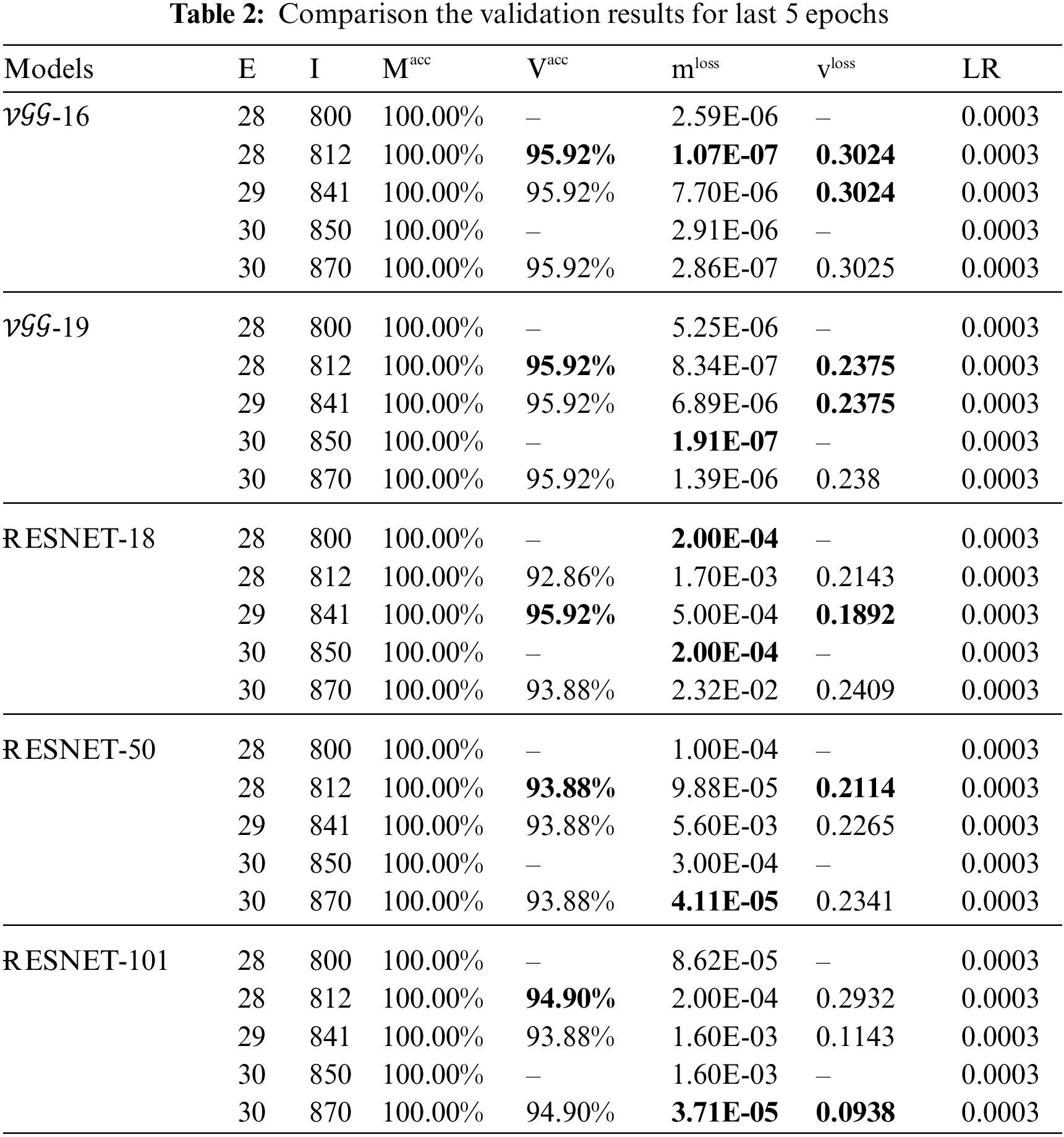
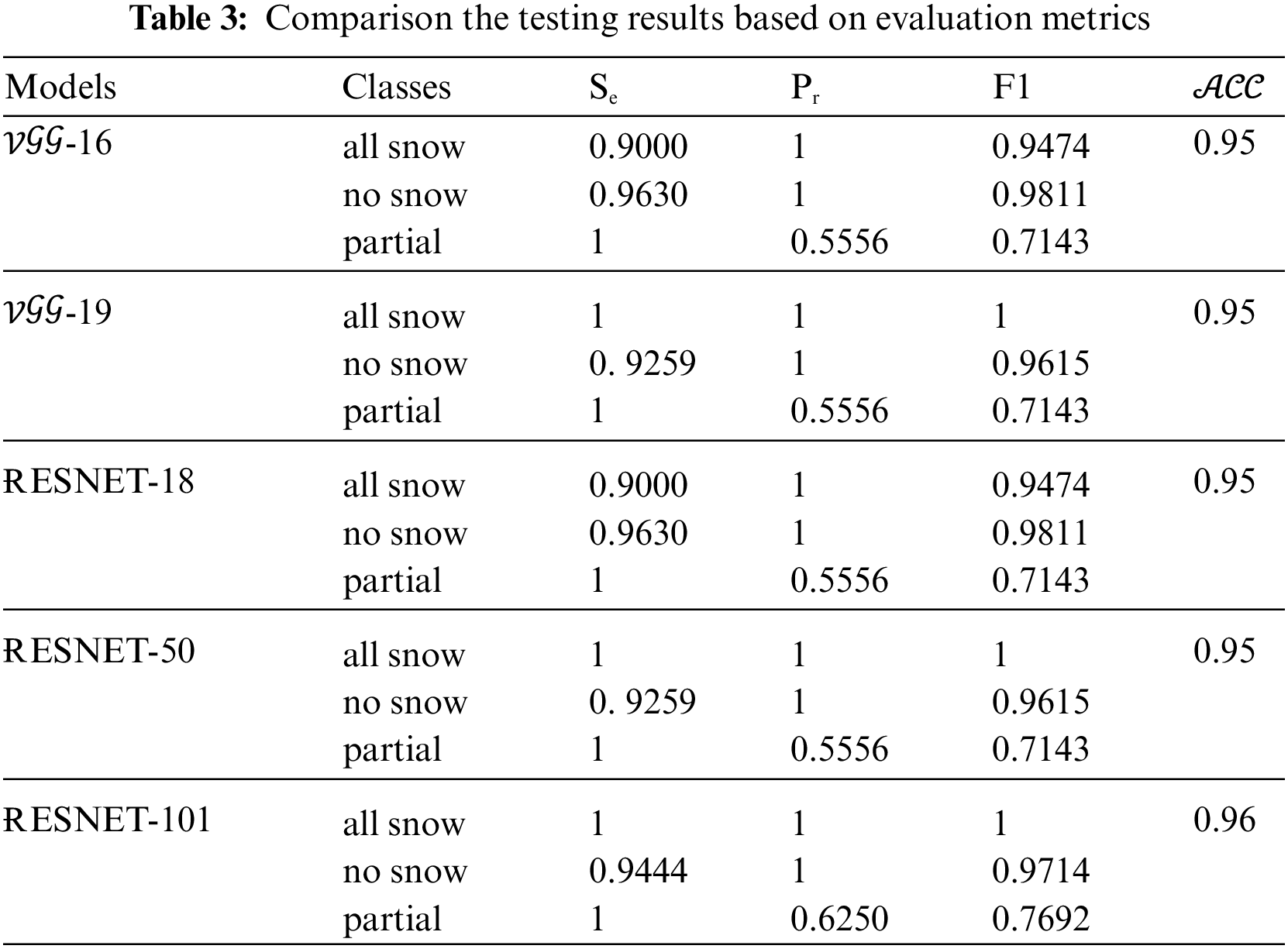
The evaluation metrics and accuracies for the testing that are used to determine the level of model quality are presented in Table 3. The VGG-16 achieves an accuracy of 0.95, whereas the overall sensitivity is recorded as 0.9543, the overall precision attained using VGG-16 is 0.8519 and the overall F1-score is recorded as 0.9002. The VGG-19 achieves an accuracy of 0.95, whereas the overall sensitivity is recorded as 0.9753, the overall precision attained using VGG-19 is 0.8519 and the overall F1-score is recorded as 0.9094. The ɌESNET-18 achieves an accuracy of 0.95, whereas the overall sensitivity is recorded as 0.9543, the overall precision attained using ɌESNET-18 is 0.8519 and the overall F1-score is recorded as 0.9002. The ɌESNET-50 achieves an accuracy of 0.95, whereas the overall sensitivity is recorded as 0.9753, the overall precision attained using ɌESNET-50 is 0.8519 and the overall F1-score is recorded as 0.9094. The ɌESNET-101 achieves an accuracy of 0.96, whereas the overall sensitivity is recorded as 0.9815, the overall precision attained using ɌESNET-101 is 0.8750 and the overall F1-score is recorded as 0.9252.

When evaluating the models, it is essential to utilize a variety of different metrics evaluation. This is due to the fact that the performance of a model may be satisfactory when using one measurement from one metric of evaluation, but it may be unsatisfactory when using another measurement from another metric of evaluation. It is essential to use evaluation metrics in order to ensure that your model is functioning correctly and to its full potential.

A confusion matrix is a table used to show the performance and effectiveness analysis of the classification model. The evaluation performance of a classification model can be represented graphically and summarized using a confusion matrix. Fig. 10 shows that the proposed solar panels classification models are evaluated using confusion matrix-based performance metrics. The confusion matrix includes actual classes and predicted classes by displaying the values of true positive, true negative, false positive, and false negative. Moreover, through these values, the sensitivity, specificity, precision, and overall accuracy metrics can be calculated. Consequently, the comparison results for our models can be seen in Fig. 10e where the ɌESNET-101 metrics outperform those of the compared models by providing more accurate diagnostic performance on the solar panels dataset. Regarding sensitivity, the results grow higher than the loss functions of other models, showing the learning effect of ɌESNET-101 on the features of each class.

Figure 10: Confusion matrix results (a) VGG-16, (b) , (c) ɌESNET-18, (d) ɌESNET-50, and (e) ɌESNET-101

Fig. 11a shows the results of VGG-16 model, where only four labels from all_snow and no_snow classes are missed to classify. Fig. 11b gives the results of VGG-19 model; it shows the missed classified labels are from no_snow class. Fig. 11c shows the achieved results by ɌESNET-18, the model struggle from the same issues in VGG-16, also four labels are missed (all_snow and no_snow classes). Fig. 11d represents the results obtained by ɌESNET-50; the same thing, four labels are missed in the no snow class. Finally, Fig. 11e presents the best result achieved by ɌESNET-101. It gives highest accuracy with 0.9694 less missing classification. Taking into account that the result was compared in the confusion matrix with 20% out of the conducted datatset.

Figure 11: Predicted distribution over classes of the compared models (a) VGG-16, (b) VGG-19, (c) ɌESNET-18, (d) ɌESNET-50, and (e) ɌESNET-101

In the second proposed approach, the upsampling method is applied to the imbalance classes with minority samples. The partial class in the conducted dataset suffers from inadequate knowledge that could provide better prediction performance. This can be accomplished by using a variety of techniques, such as rotating and inverting the images. The dataset upsampling process aims to increase the variability and uniformity of the CNN models. This procedure aids the models in learning more about the input space. Also in this approach, we simulate the challenges faced by surveillance cameras while detecting the condition of solar panels. To simulate that we applied motion blur on the original dataset with linear motion across 21 pixels at an angle of 11 degrees.

The balanced dataset is trained using the five implemented models. The accuracy and loss results of VGG-16,VGG-19, ɌESNET-18, ɌESNET-50, and ɌESNET-101 as shown in Figs. 12a and 12c. VGG-16 is more stable with less fluctuation than VGG-19 from a learning behavior perspective, it converges faster and reaches the steady-state at an earlier stage of iterations (100 iterations), furthermore, VGG-19 reaches the stability after 150 iterations. The learning behavior of ɌESNET-101 outperforms ɌESNET-18 and ɌESNET-50 architectures by achieving steady-state results with 80 iterations.

Figure 12: Second case comparison results of accuracy and losses for, VGG-16, VGG-19, ɌESNET-18, ɌESNET-50, and ɌESNET-101 based on (a) Training accuracy, (b) Validation accuracy, (c) Training losses, (d) Validation losses

The other part of the dataset is validated with 20%. The same with the first section of this experiment, the validation is performed after every 26 iterations for all models used in the analysis. As used for the validation process, it does not involve underfitting and overfitting. The obtained accuracies of validation for all models are shown in Fig. 12b, the accuracies are improving iteratively with the time. The minimum and maximum accuracies for VGG-16 are 58.62%, 100%, and VGG-19 are 39.08%, 100%, while, the median and mode for VGG-16 are 100%, 100%, and VGG-19 are 100%, 100%, respectively. The minimum and maximum accuracies for ɌESNET-18 are 33.33%, 100%, ɌESNET-50 are 51.72%, 100%, and ɌESNET-101 are 73.56%, 100%. In addition, the median and mode for ɌESNET-18 are 98.85%, 100%, ɌESNET-50 are 98.85%, 98.85%, and ɌESNET-101 are 100%, 100% respectively. Fig. 12d shows the loss results confirm the validation accuracy results, where the loss of VGG-19 suffers from a high fluctuation at the beginning of learning.

The analysis was conducted again after we applied the additions mentioned above. We found that the trio VGG-16, ɌESNET-50, ɌESNET-101 and achieved excellent classification performance than the VGG-19 and ɌESNET-18. Considering the parameter efficiency of VGG-19 and ɌESNET-18, They achieved a satisfactory performance compared to the first proposed approach.

By comparing Figs. 9 and 12 it obviously found that the upsampling increased stability of the training and validation process. During the training, the fluctuations continued almost to the end of the training, as we see in Fig. 9a, while in the second case the fluctuations stopped at 600 iterations, as we see in Fig. 12a during validation, the accuracy raised above 0.90 after 100 iterations where the accuracy fluctuations were limited between 0.97 and 1 as we see in Fig. 9b, while the accuracy was fluctuations limited between 0.90 and 1 as we see in Fig. 12b.

To determine the level of model quality, the evaluations, metrics, and testing accuracies for all models are included in Tables 4 and 5. These are used to determine how well the model is constructed. The quantitative results are well presented in Tables 4 and 5, the numerical results and the evaluation metrics of all compared architectures for the second proposed approach are clearly discussed. The experiment runs with 30 epochs, 780 iterations (for each epoch (E) 26 iterations (I)), and mini-batch accuracy (Macc) results for the last 5 epochs is 100%. The best validation accuracy (Vacc) is 100% obtained from VGG-16,VGG-19, ɌESNET-18, ɌESNET-50, and ɌESNET-101. The lowest mini-batch loss (mloss) is 4.7684E-08 obtained by ɌESNET-101, whereas the loss validation (vloss) obtained from VGG-16, is 7.6849E-05. The learning rate (LR) for all the architectures is 0.0003.

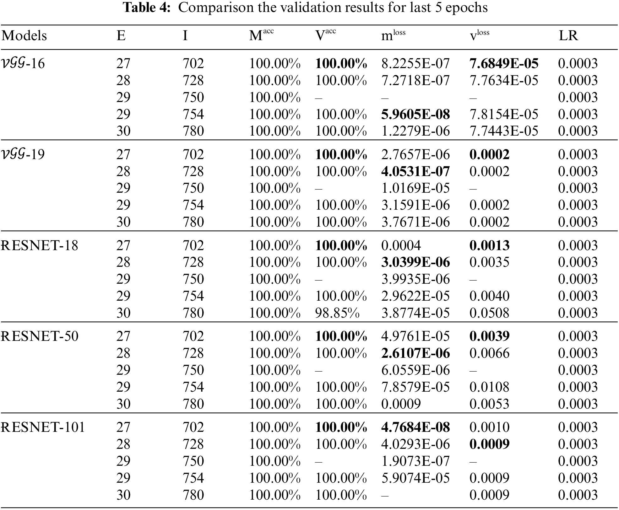
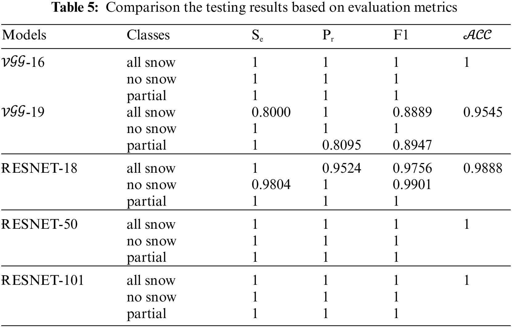
In addition, the VGG-16 achieves an accuracy of 100%, whereas the overall sensitivity is recorded as 100%, the overall precision attained using VGG-16 is 100% and the overall F1-score is recorded as 100%. The VGG-19 achieves an accuracy of 0.9545, whereas the overall sensitivity is recorded as 0.9333, the overall precision attained using VGG-19 is 0.9365 and the overall F1-score is recorded as 0.9349. The ɌESNET-18 achieves an accuracy of 0.9886, whereas the overall sensitivity is recorded as 0.9935, the overall precision attained using ɌESNET-18 is 0.9841 and the overall F1-score is recorded as 0.9888. The ɌESNET-50 achieves an accuracy of 100%, whereas the overall sensitivity is recorded as 100%, the overall precision attained using ɌESNET-50 is 100% and the overall F1-score is recorded as 100%. The ɌESNET-101 achieves an accuracy of 100%, whereas the overall sensitivity is recorded as 100%, the overall precision attained using ɌESNET-101 is 100% and the overall F1-score is recorded as 100%.

Fig. 13 shows that the diagonal matrix represents a true positive that the model has correctly predicted class dataset values; moreover, the values that are biased from the diagonal matrix are false predicted values. In addition, Fig. 13a shows there are no objects were missed in the classes. Fig. 13b gives the accuracy of VGG-19 is 0.9545, and only four missed classified objects by all snow classes. Fig. 13c ɌESNET-18 is 0.9888 by losing one object in the no snow and class. Figs. 13d and 13e verified the table results of ɌESNET-50 and ɌESNET-101 as giving 100% accuracies. Taking into account that the result was compared in the confusion matrix with 20% out of the conducted dataset.

Figure 13: Confusion matrix results (a) VGG-16, (b) VGG-19, (c) ɌESNET-18, (d) ɌESNET-50, and (e) ɌESNET-101

Fig. 14 represents the data distribution over the classes; it shows which class gives high-performance prediction and which class struggles from noise and outlier. Each of the tested models achieves different data distribution or classification. In this figure, the classes are presented in the form of a histogram. Each bar contains part of the data (class). Fig. 14a shows the predicted classes by VGG-16 model, where all classes are well predicted (no miss classification). Fig. 14b shows some of the labels from all snow classes incorrectly predicted as partial. In Fig. 14c, the case is different; some labels from no snow class are predicted as all snow classes. Figs. 14d and 14e outperform other models by achieving full classification.

Figure 14: Predicted distribution over classes of the compared models (a) VGG-16, (b) VGG-19, (c) ɌESNET-18, (d) ɌESNET-50, and (e) ɌESNET-101

In this experiment, the softmax activation function is used in the output hidden layer of tested architectures. The softmax function is used to normalize the received outputs from the previous layers by translating them from weighted sum values into probabilities that add up to one, then determine the class values. After that, the achieved probability values of the predicted classes from the output layer will be compared to the desired target. Cross-entropy is frequently used to calculate the difference between the expected and predicted multinomial probability distributions, and this difference is then used to update the model (see Eqs. (7)–(9)). Fig. 15 shows the practical investigation of this activation function.

Figure 15: Second case images probabilities with a softmax function for (a) VGG-16, (b) VGG-19, (c) ɌESNET-18, (d) ɌESNET-50, and (e) ɌESNET-101

4  Conclusion

It is very important to investigate the factors that affect solar panels and reduce their efficiency in photovoltaic energy production. One of the main factors that prevent solar panels from working properly is snowfall. The study presented five different advanced deep learning architectures in order to identify whether solar panels are coved by snow or not. The proposal incorporates five deep learning architectures that are constructed from the ground up. The investigated architectures extract meaningful features based on highly connected deep learning layers. The study performance shows how the augmented classes performed and can give appreciated results. Within the scope of this experiment, five different pre-trained models (VGG-16,VGG-19, ɌESNET-18, ɌESNET-50, and ɌESNET-101) were trained, tested, and compared regarding their overall performance. The results were conducted in two different cases, in the first case shows the comparative performance of all models tested on the original dataset without any preprocessing, then the second case simulates the extreme climate conditions by generating motion noise and how to deal with this issue; also, the dataset was replicated using the upsampling technique in order to handle the unbalancing issue. The implemented dataset was tried with two different cases; the first case was with 395 images, and for the second case, the dataset after upsampling was 437 images; for both cases, the datasets were divided into three classes, all snow, no snow, and partial. The testing accuracy results for the first case show that the VGG-16,VGG-19, ɌESNET-18, and ɌESNET-50 give the same results with 0.9592, while, ɌESNET-101 gives better testing accuracy with 0.9694. On the other hand, the learning behaviour of VGG-16, and ɌESNET-101 are more robust than the others by convergence with fewer iterations. On the other hand, in the second case, the models outperformed their counterparts in the first case by evaluating performance, where the accuracy results reached (1.00, 0.9545, 0.9888, 1.00, and 1.00) for (VGG-16,VGG-19, ɌESNET-18, and ɌESNET-50), respectively. Consequently, we conclude that the second case models outperformed their peers.

In future work, we plan to investigate other factors and apply some preprocessing and other advanced deep learning techniques.

Funding Statement: The authors received no specific funding for this study.

Conflicts of Interest: The authors declare that they have no conflicts of interest to report regarding the present study.

References

1. Yamashita, R., Nishio, M., Do, R. K. G., Togashi, K. (2018). Convolutional neural networks: An overview and application in radiology. Insights into Imaging, 9(4), 611–629. https://doi.org/10.1007/s13244-018-0639-9 [Google Scholar] [PubMed] [CrossRef]
2. Alzubaidi, L., Zhang, J., Humaidi, A. J., Al-Dujaili, A., Duan, Y. et al. (2021). Review of deep learning: Concepts, CNN architectures, challenges, applications, future directions. Journal of Big Data, 8(1), 1–74. https://doi.org/10.1186/s40537-021-00444-8 [Google Scholar] [PubMed] [CrossRef]
3. Simonyan, K., Zisserman, A. (2014). Very deep convolutional networks for large-scale image recognition. arXiv preprint arXiv:1409.1556. [Google Scholar]
4. Topbaş, A., Jamil, A., Hameed, A. A., Ali, S. M., Bazai, S. et al. (2021). Sentiment analysis for COVID-19 tweets using recurrent neural network (RNN) and bidirectional encoder representations (BERT) models. 2021 International Conference on Computing, Electronic and Electrical Engineering (ICE Cube), pp. 1–6. Quetta, Pakistan, IEEE. [Google Scholar]
5. Ahsan, M. M., Ahad, M. T., Soma, F. A., Paul, S., Chowdhury, A. et al. (2021). Detecting SARS-CoV-2 from chest X-ray using artificial intelligence. IEEE Access, 9, 35501–35513. https://doi.org/10.1109/ACCESS.2021.3061621 [Google Scholar] [PubMed] [CrossRef]
6. Xu, X., Jiang, X., Ma, C., Du, P., Li, X. et al. (2020). A deep learning system to screen novel coronavirus disease 2019 pneumonia. Engineering, 6(10), 1122–1129. https://doi.org/10.1016/j.eng.2020.04.010 [Google Scholar] [PubMed] [CrossRef]
7. Kumari, P., Toshniwal, D. (2020). Real-time estimation of COVID-19 cases using machine learning and mathematical models–The case of India. 2020 IEEE 15th International Conference on Industrial and Information Systems (ICIIS), pp. 369–374. Ropar, India. [Google Scholar]
8. Gu, X., Chen, S., Zhu, H., Brown, M. (2022). COVID-19 imaging detection in the context of artificial intelligence and the Internet of Things. Computer Modeling in Engineering & Sciences, 132(2), 507–530. https://doi.org/10.32604/cmes.2022.018948 [Google Scholar] [CrossRef]
9. Ishengoma, F. S., Rai, I. A., Said, R. N. (2021). Identification of maize leaves infected by fall armyworms using UAV-based imagery and convolutional neural networks. Computers and Electronics in Agriculture, 184(12), 106124. https://doi.org/10.1016/j.compag.2021.106124 [Google Scholar] [CrossRef]
10. Zhu, H., Yang, L., Fei, J., Zhao, L., Han, Z. (2021). Recognition of carrot appearance quality based on deep feature and support vector machine. Computers and Electronics in Agriculture, 186(11), 106185. https://doi.org/10.1016/j.compag.2021.106185 [Google Scholar] [CrossRef]
11. Hashemi, B., Cretu, A. M., Taheri, S. (2020). Snow loss prediction for photovoltaic farms using computational intelligence techniques. IEEE Journal of Photovoltaics, 10(4), 1044–1052. https://doi.org/10.1109/JPHOTOV.2020.2987158 [Google Scholar] [CrossRef]
12. Solangi, K. H., Islam, M. R., Saidur, R., Rahim, N. A., Fayaz, H. (2011). A review on global solar energy policy. Renewable and Sustainable Energy Reviews, 15(4), 2149–2163. https://doi.org/10.1016/j.rser.2011.01.007 [Google Scholar] [CrossRef]
13. Marion, B., Schaefer, R., Caine, H., Sanchez, G. (2013). Measured and modeled photovoltaic system energy losses from snow for Colorado and Wisconsin locations. Solar Energy, 97, 112–121. https://doi.org/10.1016/j.solener.2013.07.029 [Google Scholar] [CrossRef]
14. Pawluk, R. E., Chen, Y., She, Y. (2019). Photovoltaic electricity generation loss due to snow–A literature review on influence factors, estimation, and mitigation. Renewable and Sustainable Energy Reviews, 107, 171–182. https://doi.org/10.1016/j.rser.2018.12.031 [Google Scholar] [CrossRef]
15. Andrews, R. W., Pollard, A., Pearce, J. M. (2013). The effects of snowfall on solar photovoltaic performance. Solar Energy, 92, 84–97. https://doi.org/10.1016/j.solener.2013.02.014 [Google Scholar] [CrossRef]
16. Andrews, R. W., Pearce, J. M. (2012). Prediction of energy effects on photovoltaic systems due to snowfall events. 2018 38th IEEE Photovoltaic Specialists Conference, pp. 003386–003391. Austin, Texas. [Google Scholar]
17. Hassan, Q. (2020). Optimisation of solar-hydrogen power system for household applications. International Journal of Hydrogen Energy, 45(58), 33111–33127. https://doi.org/10.1016/j.ijhydene.2020.09.103 [Google Scholar] [CrossRef]
18. Hassan, Q., Jaszczur, M., Abdulateef, A. M., Abdulateef, J., Hasan, A. et al. (2022). An analysis of photovoltaic/supercapacitor energy system for improving self-consumption and self-sufficiency. Energy Reports, 8(3), 680–695. https://doi.org/10.1016/j.egyr.2021.12.021 [Google Scholar] [CrossRef]
19. Guo, X., Yang, Y., Feng, S., Bai, X., Liang, B. et al. (2022). Solar-filament detection and classification based on deep learning. Solar Physics, 297(8), 1–19. https://doi.org/10.1007/s11207-022-02019-z [Google Scholar] [CrossRef]
20. Tang, W., Yang, Q., Yan, W. (2022). Deep learning-based algorithm for multi-type defects detection in solar cells with aerial EL images for photovoltaic plants. Computer Modeling in Engineering & Sciences, 130(3), 1423–1439. https://doi.org/10.32604/cmes.2022.018313 [Google Scholar] [CrossRef]
21. Hosseini, S., Taheri, S., Farzaneh, M., Taheri, H. (2018). Modeling of snow-covered photovoltaic modules. IEEE Transactions on Industrial Electronics, 65(10), 7975–7983. https://doi.org/10.1109/TIE.2018.2803725 [Google Scholar] [CrossRef]
22. Hayibo, K. S., Petsiuk, A., Mayville, P., Brown, L., Pearce, J. M. (2022). Monofacial vs. bifacial solar photovoltaic systems in snowy environments. Renewable Energy, 193, 657–668. https://doi.org/10.1016/j.renene.2022.05.050 [Google Scholar] [CrossRef]
23. Karabuk University Provides Geographic Data Sets (2021). https://www.karabuk.edu.tr/en/ [Google Scholar]
24. Solar and Meteorological Data Sets from NASA (2021). https://power.larc.nasa.gov/ [Google Scholar]
25. Gu, J., Wang, Z., Kuen, J., Ma, L., Shahroudy, A. et al. (2018). Recent advances in convolutional neural networks. Pattern recognition, 77(11), 354–377. https://doi.org/10.1016/j.patcog.2017.10.013 [Google Scholar] [CrossRef]
26. Rasheed, J., Hameed, A. A., Djeddi, C., Jamil, A., Al-Turjman, F. (2021). A machine learning-based framework for diagnosis of COVID-19 from chest X-ray images. Interdisciplinary Sciences: Computational Life Sciences, 13(1), 103–117. https://doi.org/10.1007/s12539-020-00403-6 [Google Scholar] [PubMed] [CrossRef]
27. Zhao, X., Wei, H., Wang, H., Zhu, T., Zhang, K. (2019). 3D-CNN-based feature extraction of ground-based cloud images for direct normal irradiance prediction. Solar Energy, 181, 510–518. https://doi.org/10.1016/j.solener.2019.01.096 [Google Scholar] [CrossRef]
Cite This Article
Copyright © 2023 The Author(s). Published by Tech Science Press.
This work is licensed under a Creative Commons Attribution 4.0 International License , which permits unrestricted use, distribution, and reproduction in any medium, provided the original work is properly cited.
Downloads
Citation Tools