
 Submit a Paper
 Propose a Special lssue
 Open Access
REVIEW

Deep Learning for Financial Time Series Prediction: A State-of-the-Art Review of Standalone and Hybrid Models
1 School of Software Engineering, Xiamen University of Technology, Xiamen, 361024, China
2 Peter Faber Business School, Australian Catholic University, North Sydney, 2060, Australia
3 Department of Information Engineering, Polytechnic University of Marche, Ancona, 60121, Italy
* Corresponding Authors: Weisi Chen. Email: ; Walayat Hussain. Email:
Computer Modeling in Engineering & Sciences 2024, 139(1), 187-224. https://doi.org/10.32604/cmes.2023.031388
Received 09 June 2023; Accepted 18 September 2023; Issue published 30 December 2023
 View Full Text
 Download PDF
Abstract
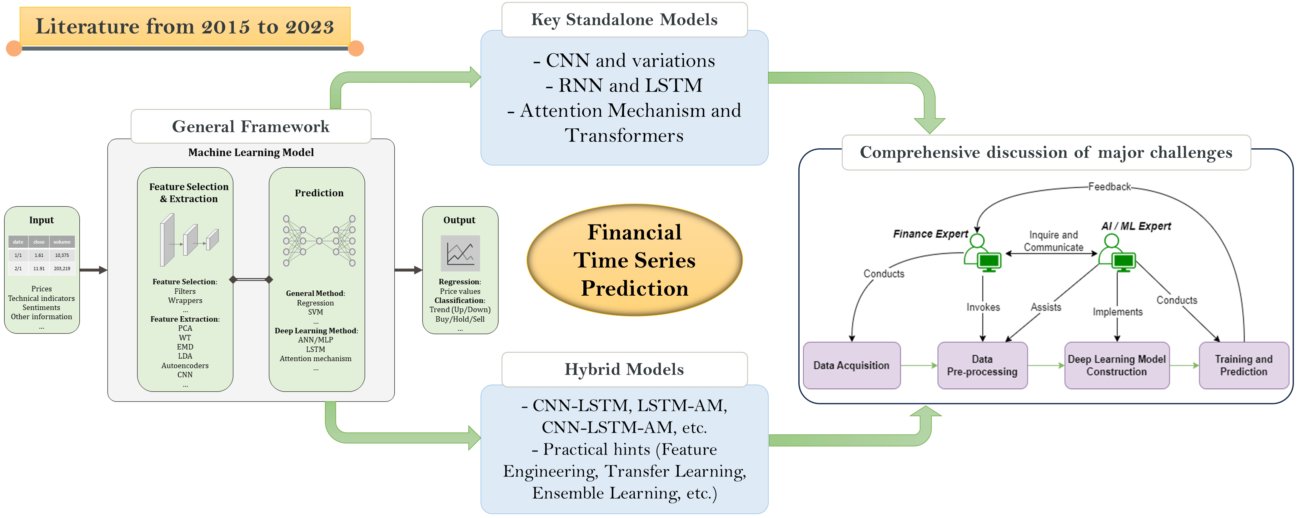
Financial time series prediction, whether for classification or regression, has been a heated research topic over the last decade. While traditional machine learning algorithms have experienced mediocre results, deep learning has largely contributed to the elevation of the prediction performance. Currently, the most up-to-date review of advanced machine learning techniques for financial time series prediction is still lacking, making it challenging for finance domain experts and relevant practitioners to determine which model potentially performs better, what techniques and components are involved, and how the model can be designed and implemented. This review article provides an overview of techniques, components and frameworks for financial time series prediction, with an emphasis on state-of-the-art deep learning models in the literature from 2015 to 2023, including standalone models like convolutional neural networks (CNN) that are capable of extracting spatial dependencies within data, and long short-term memory (LSTM) that is designed for handling temporal dependencies; and hybrid models integrating CNN, LSTM, attention mechanism (AM) and other techniques. For illustration and comparison purposes, models proposed in recent studies are mapped to relevant elements of a generalized framework comprised of input, output, feature extraction, prediction, and related processes. Among the state-of-the-art models, hybrid models like CNN-LSTM and CNN-LSTM-AM in general have been reported superior in performance to stand-alone models like the CNN-only model. Some remaining challenges have been discussed, including non-friendliness for finance domain experts, delayed prediction, domain knowledge negligence, lack of standards, and inability of real-time and high-frequency predictions. The principal contributions of this paper are to provide a one-stop guide for both academia and industry to review, compare and summarize technologies and recent advances in this area, to facilitate smooth and informed implementation, and to highlight future research directions.Graphic Abstract
Keywords
Nomenclature
| AE | Auto encoder |
| AM | Attention mechanism |
| ANN | Artificial neural network |
| AR | Autoregression |
| ARCH | Autoregressive conditional heteroscedasticity |
| ARIMA | Autoregressive integrated moving average |
| ARMA | Autoregressive moving average |
| AutoML | Automated machine learning |
| CNN | Convolutional neural network |
| DL | Deep learning |
| DPA | Direction prediction accuracy |
| DQN | Deep Q-network |
| DT | Decision tree |
| EMD | Empirical mode decomposition |
| GCN | Graph convolutional network |
| GRU | Gated recurrent unit |
| KNN | K-nearest neighbors |
| LSTM | Long short-term memory |
| MAAPE | Mean arctangent absolute percentage error |
| MACD | Moving average convergence divergence |
| MAE | Mean absolute error |
| MAPE | Mean absolute percentage error |
| ML | Machine learning |
| MLP | Multi-layer perceptron |
| MSE | Mean squared error |
| NLP | Natural language processing |
| NN | Neural network |
| O | Other data |
| OHLC | Open, high, low, close prices |
| P | Plain price data |
| PCA | Principal component analysis |
| R2 | R squared |
| RF | Random forest |
| RMSE | Root mean squared error |
| RMSRE | Root mean squared relative error |
| RNN | Recurrent neural network |
| ROC | Rate of change |
| RSI | Relative strength index |
| S | Sentiment data |
| SMA | Simple moving average |
| SVM | Support vector machine |
| TI | Technical indicator data |
| WT | Wavelet transform |
Driven by the advances of big data and artificial intelligence, FinTech (financial technology) has experienced proliferation over the last decade. One key area that FinTech is concerned with is the prices of financial market instruments, e.g., stock, option, foreign currency exchange rate, and cryptocurrency exchange rate, which are driven by market forces like the fundamental supply and demand, but in many cases extremely difficult to predict, as there is a broad range of complicated factors that may affect the prices, including macroeconomic indicators, government regulations, interest rates, corporate earnings, and profits, breaking news like COVID cases spike, company announcements like dividends, employee layoffs, investor sentiment, societal behavior, etc.
In the last decade, financial time series prediction has become a prominent topic in both academia and industry where a great many models and techniques have been proposed and adopted. These techniques can be categorized based on the linearity of the model (linear vs. non-linear) or the prediction type (regression vs. classification). Linear models include statistical analysis methods and traditional machine learning ones, such as linear regression (LR), autoregression (AR) and its variants like autoregressive moving average (ARMA), autoregressive integrated moving average (ARIMA) [1], and autoregressive conditional heteroscedasticity (ARCH), and support vector machines (SVM) [2], etc. Non-linear models include decision trees (DT), k-nearest neighbors (KNN) [3], random forests (RF) [4], support vector regression (SVR) [5], artificial neural networks (ANN) [6], and variants of ANN like multilayer perceptron (MLP), convolutional neural network (CNN) [7], and long short-term memory (LSTM) [8]. From another taxonomy perspective, some of the models are suited for regression problems (forecasting the exact future values), e.g., LR and SVR; some are appropriate for classification problems, i.e., forecasting the trend (e.g., upward or downward), e.g., SVM; whereas many other models are suitable for both types of problems, e.g., KNN, DT, RF, and deep learning models.
Before the advent and prominence of deep learning, RF, SVM, and SVR have been extensively used and were once the most effective models [9–11]. To be specific, Nikou et al. [9] explored using MLP, LSTM, SVR, and RF on the prediction of daily close prices of the UK stock market from 2015 to 2018 (a regression problem), and experiments have shown that SVR ranked second in terms of accuracy performance, with errors (namely the mean average error, the mean squared error, and the root mean squared error only higher than LSTM out of the four models. Reference [10] compared LR, RF, SVM, KNN, and MLP on stock price trends (a classification problem) and concluded that RF was top on the list in terms of accuracy. Reference [11] surveyed the literature up to 2019, and reported that SVM and RF have been two of the most adopted before the accelerated development of deep learning. Over the last decade, neural network-based deep learning has sparked heated competition in the AI world. Cutting-edge technologies like CNN, LSTM, and the attention mechanism have pushed the various domains to a new high, including computer vision, natural language processing, health data monitoring, etc. In particular, financial time series prediction performance has been elevated by these advanced deep learning models.
1.2 Characteristics of Financial Time Series Data
The enormous amount of data that the financial markets produce can be broadly divided into fundamental and market data. Fundamental data consists of details regarding the financial standing of an organization, such as earnings, revenue, and other accounting indicators. For different financial instruments, market data includes price and volume information as well as order book data that displays bid and ask levels. The interval of financial market data can be high-frequency tick-level indicating individual trades or aggregated on a daily, weekly, or monthly basis. High-frequency data offers more granular insights into market dynamics, but it also presents difficulties because of noise and abnormalities brought on by the influences of market microstructure.
Financial time series prediction is a subset of time series analysis, which in general is a challenging task. In particular, financial time series prediction involves forecasting future values of financial indicators, such as stock prices, exchange rates, and commodity prices, based on historical data. Because of their inherent complexity and specific traits, these time series pose particular difficulties for forecasting. The properties of financial time series data include, but are not limited to, the following:
1. Non-linearity and non-stationarity: Non-linearity refers to the fact that the data cannot be represented using a straight line (i.e., linearly); non-stationarity refers to the fact that their statistical properties change over time [12]. Financial time series data is known to be non-linear and often lacks stationarity due to the presence of trends, seasonality, and irregular fluctuations caused by other evolving patterns such as current affairs in the economy, shifts in investor sentiment, etc. Non-linearity and non-stationarity elevate the complexity of the data, which poses challenges when applying traditional time series analysis techniques that assume linearity or constant statistical properties over time.
2. Short-term and long-term dependencies: Financial time series have an intrinsic temporal nature as each record has dependencies, either short-term or long-term, on previous records. Short-term dependencies are concerned with intraday fluctuations and fast market movements, whereas long-term dependencies are concerned with trends and patterns that last weeks, months, or even years. It has been revealed that neglecting the temporal dependencies may result in poor prediction performance [13,14].
3. Asymmetry, fat tails, and power-law decay: Traditionally, many financial models, including some option pricing models and risk models, have relied on the assumption of normal distributions, which has been questioned by numerous researchers and financial facts in recent years. Instead, asymmetric distributions and fat-tailed behavior are often observed in financial time series, e.g., stock returns. It is empirically established that the probability distribution of price returns has a power-law decay in the tails [15,16]. This means that extreme occurrences, such as market collapses or spikes, happen more frequently than a normal distribution would suggest. Traditional models that assume normal distributions may fail to represent these exceptional events accurately.
4. Volatility: Volatility refers to the degree of variation or dispersion of a financial time series. Financial markets are known for experiencing periods of high volatility, followed by relatively calmer periods. Another phenomenon that has been observed is called volatility clustering, which occurs when periods of high volatility are followed by others with similarly high volatility, and vice versa [17]. Volatility clustering can be quantitatively defined as the power-law decay of the auto-correlation function of absolute price returns [16].
5. Autocorrelation and cross-correlation: Autocorrelation in financial time series may occur, referring to the correlation of a time series’ current values with its historical values [18]. The underlying cause could be the long-term influence of news, market sentiment, etc. Furthermore, numerous financial assets or instruments may exhibit interdependence, which is known as cross-correlation [19]. Cross-correlations between financial time series show how changes in one asset’s price affect the price of another.
6. Leverage effects: Leverage effects describe the negative relationship between asset value and volatility. It is observed that negative shocks tend to have a larger impact on volatility than positive shocks of the same magnitude [16]. In financial time series, the relationship between returns and volatility can be asymmetric, with downward movements leading to increased volatility.
7. Behavioral and event-driven dynamics: Investor behavior, sentiment, and psychological variables, as well as market-moving events such as earnings announcements, governmental decisions, geopolitical developments, and news releases, all have an impact on financial markets [20]. These behavioral and event-driven characteristics can cause significant shifts and irrational movements in financial time series.
Conventionally, effectively incorporating domain knowledge including these statistical properties into predictive models is crucial for accurate financial time series analysis and forecasting. Recently, deep learning models and hybrid approaches are being increasingly developed and employed to handle these complexities and capture the underlying dynamics of financial markets.
Note that alternative data sources, which incorporate unconventional data like sentiment from social media and web traffic patterns, have grown in popularity in recent years for the task of financial time series prediction. These alternative data sources aim to provide supplement information that may not be immediately reflected in traditional fundamental or market data.
1.3 Research Objective and Contributions
The purpose of financial time series prediction is three-fold. Firstly, for investors, it facilitates informed investment decisions, aids portfolio optimization, and ultimately maximizes profits. Research on price prediction in the literature is sometimes extended to the form of stock selection or portfolio optimization by finding the best weights for each relevant stock [21–23]. Secondly, for finance domain researchers, it provides an automated prediction process in practice and the results may contribute to financial theories. Thirdly, for data scientists, computer experts, and practitioners, it is a high-potential area where productive outcomes may be generated that can benefit both academia and industry from analytics and software perspectives.
The mainstream studies on financial time series prediction still have flaws in terms of usability, even though numerous AI researchers actively propose alternative models. Our interactions with various finance domain experts have shown a common complaint: while being the key customers of the technologies proposed for financial time series prediction, many finance domain experts lack in-depth knowledge or skills of the most cutting-edge techniques and may hesitate about where to get started, rendering the selection and deployment of these models challenging. Among so many different machine learning models out there, which algorithms are best for the given class of problems? How are they compared with each other? What methods are involved in these models and what do they imply? How can they mix and match various techniques and integrate them as components into one single model design? Currently, there is a lack of the most up-to-date review of advanced machine learning techniques for the financial time series prediction task. The motivation of this review article is to answer the forementioned questions.
This review article provides an overview of the most recent research on using deep learning methods in the context of financial time series predictions from 2015 to 2023. The principal contributions of this review article are as follows:
• Reviewing, comparing, and categorizing state-of-the-art machine learning models for financial time series prediction, with an emphasis on deep learning models involving convolutional neural networks, long short-term memory, and the attention mechanism.
• Providing a summary and a one-stop guide for finance experts and AI practitioners on selecting technology components and building the most advanced models, including the software framework, processes, and techniques involved in the practice.
• Highlighting remaining challenges and future research directions in this area.
The rest of this review article is structured as follows. Section 2 illustrates the discovery phase of the review together with some initial findings through analysis. Section 3 demonstrates the key elements and techniques involved in using deep learning in financial time series predictions, including input data, relevant feature selection and extraction techniques, and key deep learning techniques or components involved in the most recent literature. This is followed by a thorough discussion of various deep learning models adopted in the most recent literature in Section 4, mapped into a generalized deep learning framework to facilitate comparison and explanation. Finally, Section 5 concludes the paper by highlighting remaining research challenges and potential future research directions.
2 Discovery and Preliminary Analysis
2.1 Publication Source and Trend
As part of the discovery phase, we have collected a number of journal articles on applying deep learning to financial time series predictions within the Science Citation Index Expanded database by Web of Science, with a combination of keyword filters (“deep learning” combined with “financial time series”) from 2015 through 2023, and 85 journal articles were identified. SCIE is used to maintain a high-quality perspective on the literature as it tends to index only reliable sources and it excludes not peer-reviewed documents. Only journal papers have been selected as this type of article tends to be more comprehensive and detailed and provides more solid contributions. Fig. 1 shows the yearly number of publications, which indicates the upward trend of using deep learning for financial time series prediction problems. Note that no record has been found in 2015 and 2016 through this search.

Figure 1: Trend by year (2017 to 2023)
Based on a thorough examination of all the selected articles and the data involved in these research items, our initial findings are shown as pie charts in Fig. 2.

Figure 2: Initial findings: (a) percentage per problem type (classification, regression, or both); (b) percentage per financial instrument type; (c) percentage per nation of financial markets; (d) percentage per data frequency (daily or intraday)
Most of these articles dealt with the stock market, while a much smaller portion of the papers focused on other financial instruments including foreign exchange, cryptocurrency, and options. The US and Chinese stock markets have witnessed the highest popularity, which is interestingly in line with the globe-wise economic size. Some articles utilized data from multiple markets, aiming to provide a more generic and universal solution. Noticeably, daily price forecasting has been dominant in comparison with intraday forecasting (in minute-level or hour-level frequencies). The latter is often seen as a more difficult task, as the data comes in higher frequency, which brings greater data size and more complexity.
The financial price time series prediction task is primarily conducted in two forms. The first form is a classification problem, which can be binary (up or down) or 3-class classification (buy, hold, or sell) indicating the trend of the price movement; the second form is a regression problem, which focuses on forecasting the price values. It can be revealed that the selected articles distribute almost evenly in these two forms of prediction problems.
3 Elements and Techniques for Financial Time Series Predictions
In this section, we go through crucial elements and techniques involved in using deep learning for financial time series prediction tasks involved in the selected publications, including the selection of input data types, feature selection, and extraction methods, and some key relevant deep learning techniques for both training and prediction processes.
In the selected publications, the input data fed into deep learning models for financial time series prediction tasks has been acquired from a broad range of data sources of various types. The selection of input data types has a significant impact on the performance of deep learning models. Major types of data include the following, ordered by the frequency of use in the selected research works:
Plain price data. Raw features of plain price data may include basic OHLC prices (open, high, low, close), trading volume, and amount of any financial instrument, such as a cash instrument like a stock or a market index (e.g., Dow Jones, S&P 500, Nasdaq Composite, NYSE Composite in the US market and SSE index in the Chinese market); a derivative instrument like an option or a future; an exchange instrument like a currency or a cryptocurrency, etc. This type of data is sometimes referred to as fundamental indicators. The interval between data records, i.e., data frequency, can be daily or intraday (hourly, minutely, secondly, milli-secondly, etc.). Price data can be obtained directly from financial market data sources like Yahoo Finance [24] with or without data manipulation. Plain price data is fundamental for financial time series prediction problems, as it contains the price values that can be used for labeling and model evaluation. Plain price data has its presence in all selected papers, many of which have used solely plain price data as input, based on the autocorrelation property of financial time series mentioned in Section 1.3, and some have used plain price data to calculate technical indicators.
Technical indicators. Technical indicators (TI) are measures or signals generated by mathematical calculations based on plain price data (i.e., fundamental indicators). In the finance domain, TIs are commonly harnessed by investors and analysts to analyze movements of financial market time series, facilitate buy, hold, or sell decisions, or predict trends. This process is known as technical analysis (TA). In deep learning models, TI values are commonly represented as simple vectors. TIs can be acquired based on the basic values derived from the price data, or third-party data providers, and they have been reported to be effective input features for price prediction tasks and can improve prediction performance in many studies [25–28].
Based on functionality, TIs can be categorized into three categories, namely (1) trend indicators, mostly based on moving averages, signaling whether the trend direction is up or down, such as SMA (simple moving average), EMA (exponential moving average), and WMA (weighted moving average); (2) momentum indicators, measuring the strength or weakness of the price movement, such as RoC (rate of change, also known as returns in financial time series prediction, including arithmetic and logarithmic returns), stochastic oscillators (e.g., %K and %D), MACD (moving average convergence divergence), RSI (relative strength index), CCI (commodity channel index), MTM (momentum index) and WR (Williams indicator); and (3) volatility indicators, measuring the spread between the high and low prices, such as VIX (volatility index) and ATR (average true range). Practically, trend indicators Some most commonly used technical indicators in the selected publications are listed in Table 1.

Each TI is a transformation derived from the same original plain price data, focusing on a different aspect. In practice, researchers feed one or more TIs commonly seen in traditional technical analysis, with or without the original price data, into the deep learning models, and rarely give the rationale behind the TI selection. For instance, Reference [29] combined 18 TIs (covering trend indicators and momentum indicators) out of the data of six mainstream cryptocurrencies as the input for a convolutional LSTM model. Noticeably, Reference [30] has reported that using solely %K, MACD, RSI, or WR with LSTM resulted in similar accuracy (around 75%) on the FTSE TWSE Taiwan 50 Index, with MACD offering slightly higher accuracy (76%) than the other selected TIs. When combining these TIs altogether, the accuracy can reach as high as 83.6%. The result of this study suggests that (1) MACD may be able to present slightly more learnable information on the deep neural network than the other selected TIs, which, however, may not be true in all circumstances. (2) Many commonly used TIs are significantly correlated with the moving average, implying that the deep learning models may be capable of automatically filtering out the anomalies in the time series. (3) A combination of multiple TIs may contribute to enhanced accuracy.
Sentiments. Sentiment towards a particular financial instrument may influence its price movement, which has been actively studied in the finance research discipline [31]. For instance, a positive piece of news or posts on social media regarding a company may contribute to an increase in its stock price, lasting a short or longer period, and vice versa. Thus, some researchers focus on sentiment analysis of news and social media and attempt to find how these sentiments affect price movement. Such studies are mostly empirical, trying to interpret existing phenomena according to historical data. Sentiment data (typically represented as sentiment scores) can be calculated using sentiment analysis algorithms (lexicon-based or machine learning-based) or obtained directly from third-party data providers. A fairly limited number of the selected papers (e.g., [32–36]) prepared sentiment data from news and social media or used sentiments directly as part of the input data. Sentiment analysis techniques are out of the scope of the paper, and a comparison between existing methods can be found in [37].
Other information. Apart from the principal data types discussed above, any other external information that may potentially affect prices can be employed as part of the input data for financial market time series prediction tasks. Examples include new COVID cases in an area, monetary policy updates, dividend announcements, breaking news, etc. For instance, in addition to price data and technical indicators, Liu et al. [38] also included news headlines as part of the input data, preprocessed through knowledge graph embedding, which contributed to improved performance compared with traditional ML models.
Some examples of input datasets used in the selected publications are shown in Table 2. Note that in many cases, researchers may combine the data in various types from multiple sources as discussed above, to acquire a better model that can enhance prediction performance. Shah et al. For example, [39] took a broad range of input data types, including the NSE Nifty 50 stock market index price data, foreign indices, technical indicators, currency exchange rates, and commodities prices, with a sliding window of 20 trading days to predict the next day using the CNN-LSTM model. It has been reported that combined input data types may lead to enhanced performance [25].

3.2 Feature Selection and Extraction
Data used in ML can be thought of as an n-dimensional feature space, with each dimension representing a particular feature. Real-life raw data could have too many features that suffer the curse of dimensionality, highlighting the complexity and difficulty brought about by high-dimensional data. It has been reported that feeding a large number of raw features into ML gives rise to poor performance [13]. Thus, feature selection and feature extraction are often conducted before feeding data into ML models. Appropriate feature selection and extraction are known as two determinants of ML prediction performance, beneficial for the speed of ML training and meanwhile avoiding the overfitting problem.
Feature selection refers to the process of reducing the number of features, including unsupervised methods like correlation analysis, and supervised ones like filters or wrappers. The core idea is to find a subset of the most relevant features for the problem to be addressed by the ML model. Evolutionary algorithms, especially the Genetic Algorithm (GA), are sometimes chosen as a feature selection technique [42,43]. Additionally, domain-specific information could play a role in feature selection, e.g., manually selecting a subset of more critical features based on domain experts’ knowledge and experience.
Feature extraction or feature engineering is the process of transforming the raw features into a particular form that can be more suitable for modeling, commonly using a dimensionality reduction algorithm, e.g., casting high dimensional data to lower dimensional space. It is crucial to distinguish feature extraction from feature selection. The former uses certain functions to extract hidden or new features out of the original raw features, whereas the latter is focused on selecting a subset of relevant existing features. Some feature extraction techniques used in the selected literature are as follows:
Principal Component Analysis (PCA) is one of the most popular unsupervised dimensionality reduction techniques to remove unnecessary or less-important features including the noises from the input, so ML can learn more useful information from more important features. Based on singular value decomposition (SVD), the core idea of PCA is to find some principal components that form a hyperplane to look at the feature space at a different angle and have a certain percentage of the raw data projected to the hyperplane. Vanilla PCA linearly creates the hyperplane, so it is not suited for non-linear high-dimensional data. A kernel trick can be implemented to transform the data into a higher dimension so that it can be linearly separable. This is also a method commonly used in SVM. PCA with the kernel trick is also known as Kernel PCA.
Wavelet Transform (WT) is a dimensionality reduction technique broadly used for noise reduction and meanwhile maintaining the most important features of the raw data, especially in the signal processing space [44]. It is sometimes adopted in financial time series prediction tasks, e.g., di Persio et al. [45] employed both WT and PCA as feature extraction techniques built into their model.
Empirical Mode Decomposition (EMD) is a decomposition technique that goes through a sifting process breaking the raw data down into some intrinsic mode functions (IMFs) that represent distinct frequency components and a residue. For instance, Shu et al. [46,47] employed EMD and its variant, complete ensemble EMD (CEEMD) for feature extraction.
Autoencoder (AE) is a special type of ANN structure for unsupervised learning, featuring an Encoder to convert the input data into the Code in the hidden layer, and a Decoder for reconstructing the data from the Code (also known as the bottleneck) [48]. Backpropagation is used for optimizing parameters by comparing the original data and the reconstructed data. If the Code has lower dimensionality than the input data, representing the most important features of the data, the AE is called an under-complete autoencoder, which can naturally be used for dimensionality reduction. In a typical under-complete AE (Fig. 3), the Code, i.e., the compressed lower dimensional data, can further be used as input for other ML models. The idea of AE is akin to that of PCA. Essentially, if the AE’s activation function is linear inside each layer, the lower-dimensional representation at the Code corresponds directly to the principal components out of PCA. Commonly, non-linear activation functions, such as ReLU (Rectified Linear Unit) and sigmoid, are employed in AEs. More information about the activation functions will be given in Section 3.3.1.

Figure 3: An example of an under-complete autoencoder network, in which the bottleneck represents the compressed low-dimensional representation of the input
Convolutional Neural Network (CNN) was inspired by biological vision processing mechanism, has been proposed for image pattern classification initially, and then gradually adopted for prediction tasks in various fronts like speech recognition. CNN is commonly used to extract spatial features. Often, when used in financial time series, the common first step is to convert time series data into “images” before feeding it into CNN. More details about CNN will be illustrated in Section 3.3.1.
3.3 Key Deep Learning Models Involved in Financial Time Series Predictions
This section discusses key deep learning techniques commonly adopted in the selected papers on financial time series prediction, namely convolutional neural network (CNN), long short-term memory (LSTM), and attention mechanism (AM).
CNN is comprised of one or more sets of a convolution layer and a pooling layer, followed by one or more fully connected neural networks, i.e., FC layers or dense Layers. Each of the convolution layers and pooling layers consists of several feature maps, each of which represents particular features of the input data. In other words, unlike a traditional artificial neural network (ANN) where feature extraction is usually done manually, a CNN performs convolution and pooling operations for feature extraction before linking to the FC, which is typically an ANN like a Multilayer Perceptron (MLP) to generate the final prediction results.
We now illustrate the layers of a standard CNN and relevant concepts in more detail.
Convolutional Layer. A convolutional layer contains some feature maps generated by conducting the convolution operation upon the data from the preceding layer (including the input layer that represents input data). A convolution operation utilizes a filter known as convolution kernel, a matrix sliding across the input data matrix (from left to right and top to bottom) by a certain stride (the number of steps of each move of the convolution kernel, normally set as 1 by default), and carrying out inner product calculation between the kernel itself and the overlapping part of the input data matrix. Often, an operation called padding is used to add pixels/data to the frame of the data matrix, aiming to guarantee sufficient space for the convolution kernel to cover the entire matrix, which in turn enhances its performance. One common type of padding is zero padding, meaning filling additional 0’s around the frame of the original matrix. The number of convolutional layers in CNN for financial time series prediction is determined by the complexity of the features and patterns to be dealt with in the data. In practice, a common effective approach is to start with a small number of convolutional layers and gradually increase the depth. It should be noted that adding too many layers might result in overfitting, so it is critical to determine the proper balance through experimentation and validation.
Pooling Layer. The feature maps generated by each convolution layer are transformed by the pooling operation into feature maps in the subsequent pooling layer. The pooling operation, including max-pooling, average-pooling, etc. is essentially conducting data dimensionality reduction to extract the most outstanding features, reduce computation costs, and meanwhile prevent the overfitting issue. In financial time series prediction, the selection of pooling operation type should be carefully considered depending on the characteristics of the data being used. In general, either max-pooling or average-pooling can be used. However, practitioners should keep in mind that financial time series often contain complex and subtle temporal patterns that may be lost during max-pooling. Through experimentation, average-pooling or even no pooling may be selected to mitigate this issue.
Fully Connected Layer. The fully connected layer (FC), or the dense layer, is the last component of a CNN, which takes the output of former convolution layers and pooling layers as input and generates the final prediction output. The term “fully connected” indicates that all input neurons are considered by each output neuron. This layer can be implemented by one particular type of ANN, most often, an MLP, so some publications use the terms FC and MLP interchangeably in a CNN-based model. Before feeding the data into this layer, the flatten operation may be performed, which converts the output of a convolution layer into a one-dimensional vector. The number of output neurons in the final layer of CNN depends on the type of task being performed. In regression tasks, the output layer typically has a single neuron indicating the price value, whereas, in classification tasks, the output layer typically has two (upward or downward trend) or three (buy, hold, or sell) output neurons, representing the probabilities of the classes.
Activation Functions. In each neuron/perceptron of an ANN, such as the FC layer of a CNN, an activation function is in place that produces the output of that neuron based on the input. The most commonly used activation functions include sigmoid (σ), Hyperbolic tangent (tanh), and rectified linear unit (ReLU). Their formulae are shown in Eqs. (1)–(3), respectively. Vanishing gradients are a common issue of sigmoid and tanh, and ReLU has recently been a popular alternative to mitigate this issue.
For the output layer to generate the final output, a sigmoid function can be employed for binary classification, a softmax function derived from cross entropy function can be used for multi-class classification problems, as shown in Eq. (4), and a simple linear activation function may be used for regression problems.
An example of a CNN applied in daily stock price prediction (a classification problem), presented in [7], is shown in Fig. 4. In this model, a 2D matrix is created as the input data (60 days × 82 variables). The first layer uses eight filters with the size of 1 × 82 (the number of initial variables), each covering all daily variables to create higher-level features, allowing for diverse combinations of primary variables and the potential to eliminate irrelevant ones, thereby serving as an initial module for feature extraction and selection. The subfigure at the top of Fig. 4 describes how an example filter works in this scenario. The subsequent layers combine information from different days to create higher-level features representing specific time durations. The second layer uses eight 3 × 1 filters covering three consecutive days, motivated by many technical indicators that look for three-day patterns; the third layer features a 2 × 1 max-pooling operation, followed by an additional set of convolutional and pooling layers to further aggregate information across longer time intervals and generate more complex features. Finally, these features are flattened into a feature vector with 104 features, which is then used for final prediction using a fully connected layer with a sigmoid activation function that signifies the likelihood of a price increase in the market for the upcoming day.

Figure 4: An example of a typical convolutional neural network, with the illustration of a 1× the number of initial variables filter to create high-level features
While CNN has shown success in a variety of disciplines, especially computer vision, applying them to financial time series prediction involves thoughtful adaptations. Practically, experimentation and a thorough understanding of the data are required for meaningful results. Some issues when working with CNN include the following:
Data Transformation. Commonly, financial time series data can be one-dimensional. However, CNN is designed for spatial data such as images with multiple dimensions. One technique that can be used to transform one-dimensional financial time series data into an appropriate format is to create an image-like 2D dataset by running through sliding windows, or even a 3D dataset by adding the dimension of multiple markets [7].
Determining Filter Sizes. Determining convolutional kernel sizes is critical. Too small filters may overlook broader trends, whereas too large filters may neglect finer patterns. It is crucial to experiment with various sizes to determine which works best for the financial time series data.
Overfitting. Overfitting can be a problem with any neural network, including CNN. To avoid this, regularization approaches such as dropouts and early halting should be used. Dropouts essentially deactivate a portion of neurons in the particular layer, and the remaining neurons are used for the learning process. It can be applied to the input layer, or one or more hidden layers of a deep neural network. Some deep learning models proposed in the selected publications like [39] used several dropout layers.
It is worth noting a couple of variations of CNN that have been applied in financial time series prediction. The first one is the graph convolutional network (GCN), which operates on graphs [49,50]. It has been used by some for financial time series predictions [51–53]. The main difference between GCN and a standard CNN is that CNNs are designed for dealing with regular (Euclidean) structured data, while GNNs are for irregular or non-Euclidean structured data. The second one, the temporal convolutional network (TCN) [54] is a modified CNN with techniques such as casual convolutions, dilations, and padding of input sequences, to adapt to sequential data, such as natural languages and financial time series.
The recurrent neural network (RNN) has been proposed for learning based on sequences, where the order of data records matters. It enables information to persist in the hidden state acting as the “memory” remembering and utilizing precedent states, thus enabling the capture of dependencies between previous and current inputs in the data sequence. An RNN can be considered as identical repeating neural networks linked together, passing information from one to another. As shown in Fig. 5, where xt denotes the input of the repeating neural network (NN) and ht denotes the output. In a vanilla RNN, each repeating NN is a simple tanh layer. Naturally, RNN can be harnessed for sequence data and time series, in areas like speech recognition, natural language processing, and financial time series predictions.

Figure 5: The concept of a vanilla recurrent neural network (RNN)
However, vanilla RNNs suffer the issue of gradient vanishing or gradient exploding, which renders them unsuitable for longer-term dependencies. LSTM, a special kind of RNN, has emerged to address this issue [8,55]. It still follows the repeating NN (also called a “cell”) structure as described in Fig. 5, but with a more complex internal mechanism inside each cell, featuring three types of gates including the input gate, forget gate, and output gate to control the flow of information in and out of the memory cell. As shown in Fig. 6, in a typical LSTM the cell state (Ct) flows through the entire chain of LSTM, and the gates in each cell regulate the level of information to be remembered or discarded. Each gate is comprised of a sigmoid function combined with a pointwise multiplication operation and/or a tanh function. The output of the sigmoid function ranges between 0 (meaning no information is flowing through) and 1 (meaning allowing all information to go through). Three gates are involved, namely forget gate (ft), input gate (it), and output gate (ot). The relationship between these gates and the cell state (Ct) can be calculated by Eqs. (5)–(10), where W denotes the trained weight and b denotes the trained bias.

Figure 6: Inside a cell of a long short-term memory network (LSTM)
Pragmatically, RNN and LSTM can be deployed using established software tools like TensorFlow, PyTorch, and Keras. However, the following issues may occur when applying RNN and LSTM in financial time series predictions:
Gradient Vanishing. It happens when gradients get too small during backpropagation, causing learning to slow down or terminate. While LSTM was designed to address this issue, it can still occur in deep architectures or very long sequences.
Gradient Exploding. It occurs when gradients increase excessively big, possibly caused by an explosion of long-term components, resulting in unstable training. By carefully setting the network model, such as utilizing a minimal learning rate, scaling the target variables, and using a standard loss function, exploding gradients can be avoided to some extent. Some techniques such as Gradient clipping have been proposed to prevent exploding gradients in very deep networks, especially RNN. Again, LSTM was able to mitigate this issue in RNN, but it does not eliminate the problem.
Overfitting. Similar to CNN, and any neural network, RNN and LSTM may overfit the training data. Regularization techniques such as dropout and weight decay can be helpful to mitigate this issue.
Bias Amplification. RNN and LSTM may amplify biases in training data, resulting in biased predictions. It is critical to guarantee diverse and representative training data to address this challenge.
Varying Lengths of Sequences. It can be challenging to train RNN and LSTM on sequences of varying lengths. To efficiently manage sequences of varying lengths, techniques like padding, masking, and dynamic batching can be adopted.
High Computational Complexity. Long sequences can be computationally expensive to process. This problem can be mitigated with efficient implementations and hardware acceleration (e.g., GPU).
3.3.3 Attention Mechanism and Transformers
While LSTM is suitable for long-term dependencies in time series data, it may still suffer gradient vanishing or exploding on extraordinary long-term time series data. Attention Mechanism (AM) that has been a success in natural language processing (NLP) and computer vision can be extended to be applied in conjunction with RNN, LSTM, or GRU, to cope with aforementioned issues caused by overly long-term dependencies. Some successful and broadly applied AM-based models include those based on Transformers, such as BERT (Bidirectional Encoder Representations from Transformers) and GPT (Generative Pre-trained Transformer), two of the most advanced language models that have stunned the world in the past few years [56].
AM is a concept derived from neuroscience and is inspired by the cognitive mechanism of human beings. When a person observes a particular item, they generally do not focus on the entire item as a whole, with a tendency to selectively pay attention to some important parts of the observed item according to their needs. The principal goal of AM is to enhance the modeling of relationships between different elements in a sequence. In essence, AM assigns various importance weights to each part of an input sequence and extracts more critical information, so that the model is capable of dealing with long sequences and complex dependencies, and thus may result in more accurate predictions without consuming more computing and storage resources. More detail regarding AM can be found in this cornerstone article [57].
Similar to any deep learning model, AM or Transformers can be implemented using deep learning libraries such as TensorFlow and PyTorch. In addition, Hugging Face Transformers [58], a PyTorch-based library that includes pre-trained Transformer-based models with AMs may be finetuned for specific tasks such as financial time series prediction. It is an excellent starting point for understanding AM. Note that one of the beginner’s problems to be dealt with when getting started with AM is attention weights interpretation. It can be difficult to interpret the attention weights, which indicate how elements of the input sequence are being focused on by the model. Visualizing these weights can assist in interpreting what the model is paying attention to during the prediction process. TensorBoard, BertViz, Captum, and Transformers Interpret are some helpful tools that can generate interactive visualization of the attention weights and outputs of AM, which further allows the investigation of the attention process and facilitates explainable AI.
4 Deep Learning Framework and Models for Financial Time Series Predictions
For the ease of better illustration and comparison of the deep learning models in the selected papers, we employ a generalized deep learning framework for financial time series predictions that consists of a general architecture, two processes, i.e., training and prediction processes, hyperparameter tuning methods, and evaluation metrics. These are important factors that the researchers or practitioners have to determine during the design and construction of their deep learning (DL) model.
4.1.1 Architecture and Processes
The general architecture is comprised of the input, the ML model, and the output (see Fig. 7). The input data may be historical datasets or real-time data streams consisting of price data, technical indicators, sentiments, other information, or a combination of several types, as described in Section 3.1. The raw input data may be preprocessed or transformed, so it can be more suited for the selected ML model. Records in the raw or transformed input data may be labeled based on the output type for training purposes. The ML model integrates a selection of feature selection/extraction and prediction techniques organized in a particular structure. The output may be the regression-based price values, or the indication of the price movement direction, i.e., the upward or downward trend/direction to a certain degree or the corresponding buy/hold/sell signals. In practice, when building a deep learning model for financial time series predictions, researchers, developers, and finance domain experts may jointly choose the input data and the target output type, depending on their research/practical problem, as well as feature selection/extraction and DL algorithms to be adopted, and the structure these algorithms should be organized in the model design. In terms of implementation, open Python libraries such as PyTorch, TensorFlow, Keras, and Theano, or commercial tools like MATLAB are commonly used. The development relies heavily on those familiar with DL, usually IT experts rather than finance experts.

Figure 7: A general architecture for financial time series prediction
The general training process and prediction process are shown in Fig. 8.

Figure 8: General training and prediction processes for financial time series prediction models
Hyperparameters play a critical role in the performance of deep learning models in financial time series prediction [59]. Hyperparameters are essentially configuration settings for the model, such as the batch size, epochs, and the number of various neural network layers. Properly tuning these hyperparameters can lead to significant improvements in the model performance. Practitioners should select the most appropriate method based on the complexity of the search space, computational resources, and available expertise. Some commonly used hyperparameter tuning methods are illustrated as follows.
Traditional hyperparameter tuning methods include manual search, which involves manually selecting the hyperparameters based on prior experience and intuition, e.g., [60]; grid search, which systematically defines a range of values for each hyperparameter and testing all possible combinations of these values, e.g., [41]; and random search, which is akin to grid search but involves randomly sampling the hyperparameters from a predefined distribution. These methods can be effective but are either time-consuming or computationally expensive.
More advanced methods have gained increasing popularity nowadays, including Bayesian optimization which involves modeling the objective function (such as the loss function of the deep learning model) and using this model to guide the search for optimal hyperparameters; and evolutionary algorithms, such as the genetic algorithm (GA), particle swarm optimization (PSO), and artificial bee colony (ABC) that involve generating a population of hyperparameters and iteratively evolving the population based on a fitness function. These methods can quickly converge to the optimal hyperparameters. Many recent studies have employed one of these algorithms to optimize the hyperparameters of their proposed model for financial time series prediction. For instance, Chung et al. [61] employed GA to optimize hyperparameters in a CNN-only model for stock price movement prediction, including the number of convolutional kernels, the kernel size, and the pooling window size for the pooling layer; Kumar et al. [62,63] leveraged PSO and ABC respectively to evolve and optimize hyperparameters in an LSTM-only model for stock price prediction.
Many various statistical metrics have been employed in the selected publications (see Table 3) to assess the performance of their proposed models. Most commonly, accuracy, precision, recall/sensitivity, and F Measure (also called F1-score), etc., have been used for classification; mean absolute error (MAE), mean absolute percentage error (MAPE), mean arctangent absolute percentage error (MAAPE), mean squared error (MSE), root mean squared error (RMSE), root mean squared relative error (RMSRE), R squared (R2) and direction prediction accuracy (DPA), etc., have been used for regression. In addition, the training time and the prediction time of the model on CPU or GPU are sometimes also included in the comparison between models. Note that Table 3 is by no means an exhaustive list of all evaluation metrics, and more discussions on available metrics can be found in [64–66].

The rest of Section 4 will classify and discuss models used in the selected publications, mapped to elements of this general framework, highlighting their commonalities and differences. Section 4.2 focuses on standalone models including CNN-only and LSTM-only models, whereas Section 4.3 demonstrates hybrid models where CNN, LSTM, and other mechanisms are integrated and organized in various ways.
In this section, we discuss standalone models comprised of solely CNN or LSTM. Standalone traditional machine learning models like random forest (RF) or support vector machine (SVM), and basic deep learning models like ANN, are out of the scope of the paper.
A CNN-only model has solely CNN involved in the model structure. It can also be considered as a CNN-MLP or CNN-FC model as this model consists of CNN responsible for feature extraction and in most cases connected to a fully connected layer (often a basic ANN like MLP) for prediction. The CNN-only model has been used on the stock market, foreign exchange market, and cryptocurrency for both regression and classification problems. For example, Lin et al. [67] used this model for stock price trend prediction (classification); and Liu et al. [68] used this model for foreign exchange rate value predictions (regression), which reportedly outperformed ANN, SVM, and GRU.
Raw financial time series are often pre-processed or transformed to satisfy the requirement of CNN. References [68–70] transformed raw data into 2D so it can be more easily fed into CNN. In particular, Sezer et al. [70] explicitly demonstrated how technical indicator input data is transformed into 2D image representations before feeding into a CNN model for a three-way classification (Buy/Hold/Sell).
The CNN-only model has been reported to outperform traditional standalone models like SVM, linear regression, logistic regression, KNN, DT, RF [28,71], and ANN [7].
An ensemble CNN model contains multiple parallel paths of CNNs extracting features from distinct datasets, and combining the output using a function (e.g., a simple or weighted average function) from all paths to get a collective performance.
For instance, Gunduz et al. [69] proposed CNN-Corr which contains two parallel streams of convolution and pooling layers for intraday stock price movement predictions (up or down trend) on the Turkish market, highlighting the positive effect brought by reordering features based on feature correlations. Reference [72] applied ensemble CNN with multiple CNNs handling multiple 1D time series data over time intervals in parallel. Based on the assumption that financial time series prediction does not have to be always 100% accurate, Ghoshal et al. [73] customized ensemble CNN with confidence threshold to the classification output layer. In light of the market’s impact on individual stock price movement, Chen et al. [51] proposed an improved version of CNN-Corr, called GC-CNN (see Fig. 9), which combines two variants of CNNs namely GCN and dual-CNN (an ensemble CNN with two paths). It first utilizes Spearman rank-order correlation to discover several relevant stocks representing the market information in conjunction with the target stock and generates two sets of 2D images, respectively, which are then processed by GCN and dual-CNN separately, and finally, the features extracted from both paths are joint together before feeding into the FC layer.

Figure 9: Ensemble CNN model used in [51], mapped with the general architecture in Fig. 7
As discussed in Section 3.3.2, LSTM has been proposed to cope with long-term temporal dependencies in the data, which is suited for financial time series prediction tasks. Due to its broadly successful application, LSTM and its variants have emerged to be the dominant type of RNN on various fronts since its first appearance. Naturally, it can be seen in the selected publications that LSTM has become the de-facto “should-have” component in many financial time series prediction models, leveraging its capabilities of handling temporal dependencies. A fair number of studies used merely LSTM-only models for financial time series predictions [63,74–77].
Note that there are numerous variations of LSTM. First of all, looking at the ratio of the input and output items, there are various sequence prediction models in LSTM, including one-to-one, one-to-many, many-to-one, and many-to-many models. Secondly, at the cell level, the structure and functions used in each cell may vary, e.g., peephole LSTM [78] and Gated Recurrent Unit (GRU) [79]. In particular, GRU has been one of the most prominent variants and has proven equally effective as a standard LSTM [80]. Last but not least, there are architecture-wise variations, i.e., organizing LSTM in diverse ways, including stacked LSTM that has LSTM layers stacked on top of one another, bi-directional LSTM (BiLSTM) that enables both forward and backward learning, etc.
There has been no consensus on how the LSTM-only model would compare with the CNN-only model, as the prediction performance has varied in different scenarios. Some researchers compared standalone models and concluded that CNN-only performed better than LSTM-only, Stacked-LSTM, Bidirectional-LSTM (BiLSTM) [28,71] and GRU [68] for daily stock price prediction (regression); while on the contrary, Kamalov [81] claimed that LSTM-only outperformed CNN-only, MLP, and SVR using 10 years of daily stock price data of four US companies, for a classification type of prediction; and Fathali et al. [82] reported that LSTM-only outperformed CNN-only and RNN for a regression problem on NIFTY 50 stock prices.
Recently, hybrid models, combining multiple deep learning or machine learning models in an organized structure, have gained increasing popularity among researchers [83]. By leveraging the capabilities and benefits of various neural network architectures, hybrid models are designed to improve prediction accuracy. In particular, CNN is capable of extracting local features and patterns from the input financial time series, which is beneficial for modeling short-term fluctuations; LSTM excels at processing feature-rich information to capture long-term dependencies such as market trends and cycles; and AM may further enhance the model's capability to attend to relevant periods and features by dynamically focusing on different parts of the input sequence during different prediction steps, allowing it to effectively respond to market fluctuations. This section discusses some representative hybrid models in the literature.
The CNN-LSTM hybrid model is the most adopted one among all the selected recent research articles and has become one of the state-of-the-art methods. In CNN-LSTM, CNN is responsible for spatial feature extraction, and LSTM is responsible for handling temporal dependencies and conducting the time series prediction tasks.
In most cases, CNN is followed by LSTM in the model design, e.g., [29]. However, there are variations of this hybrid, utilizing CNN for dedicated types of data in parallel with LSTM. For example, [32] used price data to calculate technical indicators, and used CNN for sentiment analysis on textual data from financial news and stock forum posts, and the combined result is fed into LSTM for the actual time series prediction, so in essence, this can be classified as an LSTM only solution. Reference [84] proposed a similar approach with a slight distinction, where news headlines were processed by CNN and price data is processed by LSTM, the outputs of CNN and LSTM were then combined to give the final result using compensation formulae.
CNN-LSTM in most scenarios outperforms standalone models like CNN-only and LSTM-only. Reference [29] focused on intraday cryptocurrency exchange trend prediction (classification), using price data and technical indicators as input, and CNN-LSTM as the model. It has been reported that the model by far beat other baseline models including CNN-only and MLP. Reference [85] used limit order book data for stock price prediction (both classification and regression). Before the CNN-LSTM model, an LSTM-based autoencoder was applied as part of feature extraction. Reference [41] used a CNN-LSTM model on 14 years of USD/CNY foreign exchange data plus the closing price of key market indices to predict USD/CNY and the LSTM used was a modified version of LSTM called TLSTM that adds the 1-tanh function following the input gate of a traditional LSTM, aiming to retain important features of the input data to an optimal level. It outperformed MLP, CNN, RNN, LSTM, and traditional CNN-LSTM in the defined scenario. Reference [86] adopted a CNN-LSTM model for option prediction. References [46,87] utilized CNN-LSTM for daily stock data, and Hou et al. [52] used it for intraday stock data. Fig. 10 demonstrates the CNN-LSTM model presented in [87].

Figure 10: CNN-LSTM model used in [87], mapped with the general architecture in Fig. 7
Researchers have made efforts to enhance CNN-LSTM with variants of CNN or LSTM. For instance, Wang et al. [88] proposed a CNN-BiSLSTM model for stock price value prediction (regression), using an improved version of BiLSTM having a 1-tanh function added to the output gate. This model was reported to be superior to MLP, RNN, LSTM, BiLSTM, CNN-LSTM, and vanilla CNN-BiLSTM in the defined scenario. A variant of LSTM called ConvLSTM is applied in [89] for stock price value prediction using CNN-LSTM. ConvLSTM vs vanilla LSTM is akin to CNN vs. ANN, with convolution operations in place of internal matrix multiplications, aiming to keep the 3D spatial-temporal data structure rather than a 1D vector throughout the network.
As discussed in Section 3.3.3, the attention mechanism (AM) has recently emerged to handle excessively long-term dependencies. LSTM-AM and CNN-LSTM-AM models are emerging trending models, introducing the power of AM in conjunction with the LSTM and CNN-LSTM models that have been discussed above. For instance, Long et al. [90] collected both stock price data and clients’ transaction data, and enabled AM to follow a bidirectional LSTM (BiLSTM) for stock price trend prediction (classification). Reference [40] applied the CNN-LSTM-AM model, Lu et al. [91,92] adopted the CNN-BiLSTM-AM model for stock price value prediction (regression). In particular, the attention mechanism used in [92] is Efficient Channel Attention (ECA), a light-weight channel attention mechanism. The performance of CNN-LSTM-AM has been reported to be superior to CNN-only and CNN-LSTM models, and thus it becomes one of the most up-to-date state-of-the-art models.
Component organization (CNN, LSTM, and AM) may vary in design. Reference [60] proposed an ensemble CNN and LSTM organized in parallel, and Ave/Max AM is applied after the concatenation of CNN outputs. The outputs of both paths are concatenated and processed by MLP for prediction results (Fig. 11). The authors have reported that when doing daily stock price predictions (regression), this model outperformed standalone ML models including RNN, CNN, LSTM, SVM, linear and logistic regression, and random forest, but they have not compared their model with other hybrid models in terms of training and test errors. Reference [93] also proposed two parallel paths in a hybrid model, named CNN Local/Global and CNN-LSTM paths, respectively, aiming to use a prepared dataset with both Twitter and price data for stock price movement prediction (classification). The CNN Local/Global path is responsible for extracting spatial features within the data and it consists of local attention and global attention layers embedded in the CNN structure; the CNN-LSTM path utilized CNN and BiLSTM, each followed by an attention layer. These two paths are then merged into a fusion center with three fully connected layers for feature concatenation and final prediction.

Figure 11: CNN-LSTM-AM model used in [60], mapped with the general architecture in Fig. 7
4.4 Discussion and Practical Hints
Standalone deep learning models like CNN and LSTM have proven to outperform traditional machine learning models like SVM and RF. Ensemble models with multiple CNNs in parallel have proven to be superior to the CNN-only model. The advantage of CNN is to extract spatial dependencies within data, and LSTM is capable of extracting temporal dependencies. It is natural to integrate them both in a way to take advantage of both benefits. In addition, the attention mechanism (AM) can handle extra long-term dependencies which are beyond the capabilities of LSTM. Thus, hybrid models like CNN-LSTM, LSTM-AM, and CNN-LSTM-AM have emerged recently. Table 4 lists some representative studies using various classification models with some of their reported methods and results. In many publications, the performance of hybrid models has been reported to be superior to standalone models in terms of accuracy.

The training and inference time of a hybrid model on a GPU is in many scenarios longer than a standalone model. In other words, hybrid models have higher complexity than standalone models. For instance, the CNN-LSTM-AM model proposed in [60] experienced approximately twice or three times longer mean training time for each epoch on a GPU than CNN, LSTM, and RNN.
It should also be noted that there are other combinations based on CNN and LSTM, e.g., CNN-SVM [95,96] leveraged CNN for feature extraction, linked to SVM for prediction on global stock market data; XGBoost-LSTM [97] adopted extreme gradient boosting for feature extraction, followed by LSTM for prediction on forex data. Reference [98] combined CNN with a reinforcement learning technique called Deep Q-Network (DQN) [99], i.e., training the model with rewards distinguishing the magnitude of price changes. Reference [38] leveraged the ARIMA model with CNN to predict USD/CNY as a regression problem, and has demonstrated that ARIMA improves the performance compared with the CNN-only model.
Incorporating hybrid models into financial time series prediction tasks necessitates a mix of domain knowledge and deep learning skills. Building trustworthy and successful models for financial time series prediction requires continuous monitoring, validation of out-of-sample data, and transparency in understanding model decisions. While hybrid models are powerful, their complicated structures make them difficult to interpret. Model predictions can be attributed back to input features using techniques such as Layer-wise Relevance Propagation (LRP) and Shapley Additive Explanations (SHAP) to facilitate explainable AI [100].
Practically, sufficient attention should be paid to the following technical aspects when leveraging deep learning models for financial time series prediction:
Data Preprocessing. In many cases, the data should be properly preprocessed and/or normalized. Techniques like differencing to make the data stationary can be considered, e.g., when modeling returns.
Feature Engineering. As mentioned in Section 3.2, feature selection and extraction are crucial to form meaningful input features that capture domain-specific knowledge. Practitioners should consider using multiple types of data including prices, technical indicators, social network data, and/or news sentiment. In addition, models trained on historical data may underperform during occurrences that deviate from historical patterns. It can be considered to continuously update the model using new data regularly.
Transfer Learning. Taking advantage of pre-trained models may facilitate useful initializations for standalone or hybrid models. Fine-tuning them on financial time series might result in enhanced performance.
Ensemble Learning. It could be helpful to combine prediction results from multiple models [101], each with different architectures or initialization, to enhance the accuracy and robustness of prediction.
Validation and Testing. Rigorous validation and back-testing can be utilized to evaluate the model’s performance. Avoid overfitting by validating on out-of-sample data.
As a summary, Table 5 compares the key models discussed in this section, accompanied by some representative references.

5 Conclusion, Challenges, and Future Directions
Financial time series prediction, whether for classification or regression, has been a heated research topic over the last decade. While traditional machine learning algorithms have experienced mediocre results, deep learning has largely contributed to the elevation of the prediction performance. Based on literature between 2015 and 2023, CNN, LSTM, CNN-SVM, CNN-LSTM, and CNN-LSTM-AM are considered to be state-of-the-art models, which have beaten traditional machine learning methods in most scenarios. Among these models, hybrid models like CNN-LSTM and CNN-LSTM-AM have proven superior to stand-alone models in prediction performance, with the CNN component responsible for spatial feature extraction, the LSTM component responsible for long-term temporal dependencies, and AM handling overly long-term dependencies. This paper provides a one-stop guide for both academia and industry to review the most up-to-date deep learning techniques for financial market price prediction, and guide potential researchers or practitioners to design and build deep learning FinTech solutions. There are still some major challenges and gaps, which lead to future work directions.
Challenge 1: non-friendliness for finance domain experts. The process of using deep learning for financial time series predictions is overall too complicated for finance experts without IT expertise, so the dominant approach for them to conduct prediction tasks is either to communicate the requirements with IT experts for programming assistance or to learn a specific data analytics tool or programming languages themselves, which is either fairly involving or challenging (see Fig. 12). Most of the existing research merely concentrates on the deep learning model itself and its prediction performance, overlooking the usability for finance domain experts. Automatic machine learning (AutoML) [114] is an emerging technology that originated from meta-learning, which can automate everything from collecting data to deploying machine learning models, minimizing the involvement of domain experts in the construction of ML models. This can be a potential resolution to this challenge but it is still at its very early stage.

Figure 12: Common process of finance experts conducting ML-enabled financial time series predictions
Challenge 2: delayed prediction. The second significant gap is that when using only plain price data as input, the neural network predicted trend may be delayed compared with the actual trend, as can be observed from many studies [41,45]. We define this issue as “the curse of delayed prediction” (see Fig. 13), which essentially makes the prediction lack forward-looking capabilities and merely follow the actual trend. One of the underlying reasons is the Efficient Market Hypothesis, meaning the market reacts quickly to all available information, which is efficiently incorporated into price values. Introducing external information like sentiments and breaking news as input could potentially improve it to some extent, but there is currently no systematic method to achieve this. Most of the existing work selected either solely the plain price data or several technical indicators without providing much underlying rationale. This also reflects the lack of communication between AI experts and finance domain experts, leading to the third challenge–domain knowledge negligence–to be explained. Ideas from other domains may inspire new solutions. For instance, the Smith predictor is a predictive control model aiming to overcome process dead time or delay [115]. FinTech practitioners may consider applying a similar mechanism to compensate for the time delay by using an approximated model. It should be noted that while financial markets are complicated and dynamic, and forecasting exact short-term price fluctuations with high precision is extremely difficult, these deep learning models may still provide useful insights into broader trends and patterns, which can facilitate trading strategies and investment decisions. Some innovations can be made on what to predict. For instance, some research work found that market volatility is more predictable than price values [116].

Figure 13: The curse of delayed prediction: the predicted values are following the actual trend without forward-looking capabilities
Challenge 3: domain knowledge negligence. Which input data types or a combination of them may work best? In what financial contexts? These are the unanswered questions. From another perspective, this reflects that domain knowledge is largely neglected. For example, sentiments, one of the key factors of price movement, are not sufficiently harnessed to their full potential, with only a small portion of the publications using them. A systematic approach to the incorporation of finance domain knowledge into deep learning methods is in need. To address this issue, the following techniques could be attempted. First, multiple data types, especially those with rich financial insights (e.g., technical indicators and market sentiment), can be encapsulated into features. A thorough comparison of various combinations of different types of data using deep learning models is needed to guide what combination may work best. Second, financial concepts can be incorporated into the model's architecture, e.g., by adding embedding layers that represent asset types, technical indicators, or industry sectors, which can be beneficial for capturing hierarchical relationships and similarities between financial concepts. Third, transfer learning mentioned in Section 4.4 can be used to take advantage of finance-oriented pre-trained models. Fourth, rule-based AI can be leveraged to incorporate well-established knowledge as rules (e.g., more recent data is given more weight [117]). The rules can be combined with deep learning models to enhance performance. Last but not least, loss functions can be specifically customized to align with financial objectives for the defined financial time series prediction problem.
Challenge 4: lack of standards. Standard datasets and benchmarks are currently lacking. Most of the selected studies used a distinct dataset, in a different market, over a different selection of period and length. A model superior in one scenario may be inferior in another. The establishment of standards that covers various types of scenarios could make it easier for the researchers to evaluate their models and make comparisons.
Challenge 5: real-time and high-frequency prediction. Most existing studies have only used historical daily data. Among the limited number of studies using intraday data, it has only been at the minute or hourly level. When it comes to real-time analytics, would the existing models still work on incoming data streams when huge amounts of data continuously arrive? For example, when there is breaking news affecting a certain financial instrument, can the model react immediately with minimal latency? Delayed responses may lead to unexpected financial loss. Real-time analytics is a field that has been attracting growing attention [118,119]. A potential resolution is to leverage the real-time handling power of complex event processing by enabling real-time pattern detection and continual learning [14], while this remains challenging as insufficient research has been done in the real-time space. In addition, data with higher frequency (e.g., in milliseconds) may bring in more problems when using the existing deep learning models. Other research disciplines such as high-energy physics have attempted to deal with high-frequency events using techniques like event selection, aggregation, and statistical sampling. For instance, some physical events like high energy particle collisions occur at a very high rate, which makes it impossible to save all of the events to disk. Thus, a selection trigger can be used to select noteworthy events by reducing the recorded events to an acceptable number [120]. Such ideas can be borrowed by the FinTech community. Future research in this direction, including but not limited to model design, software architecture, and hardware upgrade, is more than necessary to make financial time series prediction more practical and can be used by researchers and investors with more confidence.
Acknowledgement: We acknowledge the ongoing support provided by Prof. Fethi Rabhi and the FinanceIT research group of UNSW Sydney.
Funding Statement: This research was funded by the Natural Science Foundation of Fujian Province, China (Grant No. 2022J05291) and Xiamen Scientific Research Funding for Overseas Chinese Scholars.
Author Contributions: The authors confirm the contribution to the paper as follows: study conception and design: W. Chen, W. Hussain; data collection: W. Chen, W. Hussain; analysis and interpretation of results (for the reviewed publications): W. Chen, F. Cauteruccio, X. Zhang; draft manuscript preparation: W. Chen, W. Hussain, X. Zhang; revised manuscript preparation: W. Chen, W. Hussain, F. Cauteruccio. All authors reviewed and approved the final version of the manuscript.
Availability of Data and Materials: The articles surveyed in this paper can be found in mainstream indexing databases. The list of reviewed papers and relevant analysis data can be made available by the authors upon request.
Conflicts of Interest: The authors declare that they have no conflicts of interest to report regarding the present study.
References
1. Li, Z., Liao, Y., Hu, B., Ni, L., Lu, Y. (2022). A financial deep learning framework: Predicting the values of financial time series with ARIMA and LSTM. International Journal of Web Services Research, 19(1), 1–15. [Google Scholar]
2. Gupta, D., Pratama, M., Ma, Z., Li, J., Prasad, M. (2019). Financial time series forecasting using twin support vector regression. PLoS One, 14(3), e0211402. [Google Scholar] [PubMed]
3. Latha, R. S., Sreekanth, G. R., Suganthe, R. C., Geetha, M., Selvaraj, R. E. et al. (2022). Stock movement prediction using KNN machine learning algorithm. Proceedings of the 2022 International Conference on Computer Communication and Informatics (ICCCI), pp. 1–5. Coimbatore, India. [Google Scholar]
4. Omar, A. B., Huang, S., Salameh, A. A., Khurram, H., Fareed, M. (2022). Stock market forecasting using the random forest and deep neural network models before and during the COVID-19 period. Frontiers in Environmental Science, 10. https://doi.org/10.3389/fenvs.2022.917047 [Google Scholar] [CrossRef]
5. Jiang, H., Wang, Z. (2010). GMRVVm-SVR model for financial time series forecasting. Expert Systems with Applications, 37(12), 7813–7818. [Google Scholar]
6. Vui, C. S., Soon, G. K., On, C. K., Alfred, R., Anthony, P. (2013). A review of stock market prediction with artificial neural network (ANN). Proceedings of the 2013 IEEE International Conference on Control System, Computing and Engineering, pp. 477–482. Penang, Malaysia. [Google Scholar]
7. Hoseinzade, E., Haratizadeh, S. (2019). CNNpred: CNN-based stock market prediction using a diverse set of variables. Expert Systems with Applications, 129, 273–285. [Google Scholar]
8. Hochreiter, S., Schmidhuber, J. (1997). Long short-term memory. Neural Computation, 9(8), 1735–1780. [Google Scholar] [PubMed]
9. Nikou, M., Mansourfar, G., Bagherzadeh, J. (2019). Stock price prediction using deep learning algorithm and its comparison with machine learning algorithms. Intelligent Systems in Accounting, Finance and Management, 26(4), 164–174. [Google Scholar]
10. Ballings, M., van den Poel, D., Hespeels, N., Gryp, R. (2015). Evaluating multiple classifiers for stock price direction prediction. Expert Systems with Applications, 42(20), 7046–7056. [Google Scholar]
11. Kumbure, M. M., Lohrmann, C., Luukka, P., Porras, J. (2022). Machine learning techniques and data for stock market forecasting: A literature review. Expert Systems with Applications, 197, 116659. [Google Scholar]
12. Schmitt, T. A., Chetalova, D., Schäfer, R., Guhr, T. (2013). Non-stationarity in financial time series: Generic features and tail behavior. Europhysics Letters, 103(5), 58003. [Google Scholar]
13. Rabhi, F. A., Mehandjiev, N., Baghdadi, A. (2020). State-of-the-art in applying machine learning to electronic trading. In: Clapham, B., Koch, J. A. (Eds.Enterprise applications, markets and services in the finance industry, pp. 3–20. Cham: Springer. [Google Scholar]
14. Chen, W., El Majzoub, A., Al-Qudah, I., Rabhi, F. A. (2023). A CEP-driven framework for real-time news impact prediction on financial markets. Service Oriented Computing and Applications, 17(2), 129–144. [Google Scholar]
15. Aloui, C., Hamida, H. B. (2014). Modelling and forecasting value at risk and expected shortfall for GCC stock markets: Do long memory, structural breaks, asymmetry, and fat-tails matter? The North American Journal of Economics and Finance, 29, 349–380. [Google Scholar]
16. Takahashi, S., Chen, Y., Tanaka-Ishii, K. (2019). Modeling financial time-series with generative adversarial networks. Physica A: Statistical Mechanics and its Applications, 527, 121261. [Google Scholar]
17. D’Urso, P., Cappelli, C., di Lallo, D., Massari, R. (2013). Clustering of financial time series. Physica A: Statistical Mechanics and its Applications, 392(9), 2114–2129. [Google Scholar]
18. Buonocore, R. J., Aste, T., Di Matteo, T. (2016). Measuring multiscaling in financial time-series. Chaos, Solitons & Fractals, 88, 38–47. [Google Scholar]
19. Zhang, N., Lin, A., Yang, P. (2020). Detrended moving average partial cross-correlation analysis on financial time series. Physica A: Statistical Mechanics and its Applications, 542, 122960. [Google Scholar]
20. Li, Q., Tan, J., Wang, J., Chen, H. (2021). A multimodal event-driven LSTM model for stock prediction using online news. IEEE Transactions on Knowledge and Data Engineering, 33(10), 3323–3337. [Google Scholar]
21. Ma, Y., Han, R., Wang, W. (2021). Portfolio optimization with return prediction using deep learning and machine learning. Expert Systems with Applications, 165, 113973. [Google Scholar]
22. Soleymani, F., Paquet, E. (2020). Financial portfolio optimization with online deep reinforcement learning and restricted stacked autoencoder–DeepBreath. Expert Systems with Applications, 156, 113456. [Google Scholar]
23. Ma, Y., Han, R., Wang, W. (2020). Prediction-based portfolio optimization models using deep neural networks. IEEE Access, 8, 115393–115405. [Google Scholar]
24. Yahoo Finance. https://finance.yahoo.com/ (accessed on 01/06 2023) [Google Scholar]
25. Chandar, S. K. (2022). Convolutional neural network for stock trading using technical indicators. Automated Software Engineering, 29(1), 16. [Google Scholar]
26. Thesia, Y., Oza, V., Thakkar, P. (2022). Predicting stock price movement using a stack of multi-sized filter maps and convolutional neural networks. International Journal of Computational Science and Engineering, 25(1), 22–33. [Google Scholar]
27. Maratkhan, A., Ilyassov, I., Aitzhanov, M., Demirci, M. F., Ozbayoglu, A. M. (2021). Deep learning-based investment strategy: Technical indicator clustering and residual blocks. Soft Computing, 25(7), 5151–5161. [Google Scholar]
28. Sim, H. S., Kim, H. I., Ahn, J. J. (2019). Is deep learning for image recognition applicable to stock market prediction? Complexity, 2019, 4324878. [Google Scholar]
29. Alonso-Monsalve, S., Suarez-Cetrulo, A. L., Cervantes, A., Quintana, D. (2020). Convolution on neural networks for high-frequency trend prediction of cryptocurrency exchange rates using technical indicators. Expert Systems with Applications, 149, 113250. [Google Scholar]
30. Lee, M. C., Chang, J. W., Hung, J. C., Chen, B. L. (2021). Exploring the effectiveness of deep neural networks with technical analysis applied to stock market prediction. Computer Science and Information Systems, 18(2), 401–418. [Google Scholar]
31. Chen, W., Al-Qudah, I., Rabhi, F. A. (2022). A framework for facilitating reproducible news sentiment impact analysis. Proceedings of the 5th International Conference on Software Engineering and Information Management (ICSIM), pp. 125–131. Yokohama, Japan. [Google Scholar]
32. Wu, S., Liu, Y., Zou, Z., Weng, T. H. (2022). S_I_LSTM: Stock price prediction based on multiple data sources and sentiment analysis. Connection Science, 34(1), 44–62. [Google Scholar]
33. Kilimci, Z. H., Duvar, R. (2020). An efficient word embedding and deep learning based model to forecast the direction of stock exchange market using twitter and financial news sites: A case of istanbul stock exchange (BIST 100). IEEE Access, 8, 188186–188198. [Google Scholar]
34. Zhang, W., Tao, K. X., Li, J. F., Zhu, Y. C., Li, J. (2020). Modeling and prediction of stock price with convolutional neural network based on blockchain interactive information. Wireless Communications and Mobile Computing, 2020, 6686181. [Google Scholar]
35. Kilimci, Z. H. (2020). Financial sentiment analysis with deep ensemble models (DEMs) for stock market prediction. Journal of the Faculty of Engineering and Architecture of Gazi University, 35(2), 635–650. [Google Scholar]
36. Liapis, C. M., Karanikola, A., Kotsiantis, S. (2023). Investigating deep stock market forecasting with sentiment analysis. Entropy, 25(2), 219. [Google Scholar] [PubMed]
37. Dang, N. C., Moreno-García, M. N., De la Prieta, F. (2020). Sentiment analysis based on deep learning: A comparative study. Electronics, 9(3), 483. [Google Scholar]
38. Liu, Y., Zeng, Q., Ordieres Mere, J., Yang, H. (2019). Anticipating stock market of the renowned companies: A knowledge graph approach. Complexity, 2019, 9202457. [Google Scholar]
39. Shah, A., Gor, M., Sagar, M., Shah, M. (2022). A stock market trading framework based on deep learning architectures. Multimedia Tools and Applications, 81(10), 14153–14171. [Google Scholar] [PubMed]
40. Song, T., Yan, X. (2021). Dynamic adjustment of stock position based on hybrid deep neural network. Journal of Ambient Intelligence and Humanized Computing, 12(11), 10073–10089. [Google Scholar]
41. Wang, J., Wang, X., Li, J., Wang, H. (2021). A prediction model of CNN-TLSTM for USD/CNY exchange rate prediction. IEEE Access, 9, 73346–73354. [Google Scholar]
42. Jadhav, S., He, H., Jenkins, K. (2018). Information gain directed genetic algorithm wrapper feature selection for credit rating. Applied Soft Computing, 69, 541–553. [Google Scholar]
43. Gao, R., Zhang, X., Zhang, H., Zhao, Q., Wang, Y. (2022). Forecasting the overnight return direction of stock market index combining global market indices: A multiple-branch deep learning approach. Expert Systems with Applications, 194, 116506. [Google Scholar]
44. Bao, W., Yue, J., Rao, Y. (2017). A deep learning framework for financial time series using stacked autoencoders and long-short term memory. PLoS One, 12(7), e0180944. [Google Scholar] [PubMed]
45. di Persio, L., Honchar, O. (2016). Artificial neural networks architectures for stock price prediction: Comparisons and applications. International Journal of Circuits, Systems and Signal Processing, 10, 403–413. [Google Scholar]
46. Shu, W., Gao, Q. (2016). Forecasting stock price based on frequency components by emd and neural networks. IEEE Access, 8, 206388–206395. [Google Scholar]
47. Rezaei, H., Faaljou, H., Mansourfar, G. (2021). Stock price prediction using deep learning and frequency decomposition. Expert Systems with Applications, 169, 114332. [Google Scholar]
48. Choudhury, A. R., Abrishami, S., Turek, M., Kumar, P. (2020). Enhancing profit from stock transactions using neural networks. AI Communications, 33(2), 75–92. [Google Scholar]
49. Zhang, S., Tong, H., Xu, J., Maciejewski, R. (2019). Graph convolutional networks: A comprehensive review. Computational Social Networks, 6(1), 11. [Google Scholar] [PubMed]
50. Soleymani, F., Paquet, E. (2021). Deep graph convolutional reinforcement learning for financial portfolio management–DeepPocket. Expert Systems with Applications, 182, 115127. [Google Scholar]
51. Chen, W., Jiang, M., Zhang, W. G., Chen, Z. (2021). A novel graph convolutional feature based convolutional neural network for stock trend prediction. Information Sciences, 556, 67–94. [Google Scholar]
52. Hou, X., Wang, K., Zhong, C., Wei, Z. (2021). ST-Trader: A spatial-temporal deep neural network for modeling stock market movement. IEEE/CAA Journal of Automatica Sinica, 8(5), 1015–1024. [Google Scholar]
53. Zhao, C., Liu, X., Zhou, J., Cen, Y., Yao, X. (2022). GCN-based stock relations analysis for stock market prediction. PeerJ Computer Science, 8, e1057. [Google Scholar] [PubMed]
54. Soleymani, F., Paquet, E. (2022). Long-term financial predictions based on feynman-dirac path integrals, deep bayesian networks and temporal generative adversarial networks. Machine Learning with Applications, 7, 100255. [Google Scholar]
55. Fang, Z., Ma, X., Pan, H., Yang, G., Arce, G. R. (2023). Movement forecasting of financial time series based on adaptive LSTM-BN network. Expert Systems with Applications, 213, 119207. [Google Scholar]
56. Birhane, A., Kasirzadeh, A., Leslie, D., Wachter, S. (2023). Science in the age of large language models. Nature Reviews Physics, 5(5), 277–280. [Google Scholar]
57. Vaswani, A., Shazeer, N., Parmar, N., Uszkoreit, J., Jones, L. et al. (2017). Attention is all you need. Proceedings of the 31st International Conference on Neural Information Processing Systems, Long Beach, California, USA. [Google Scholar]
58. Jain, S. M. (2022). Introduction to transformers for NLP: With the hugging face library and models to solve problems. USA: A Press. [Google Scholar]
59. Hoque, K. E., Aljamaan, H. (2021). Impact of hyperparameter tuning on machine learning models in stock price forecasting. IEEE Access, 9, 163815–163830. [Google Scholar]
60. Kamara, A. F., Chen, E., Pan, Z. (2022). An ensemble of a boosted hybrid of deep learning models and technical analysis for forecasting stock prices. Information Sciences, 594, 1–19. [Google Scholar]
61. Chung, H., Shin, K. S (2020). Genetic algorithm-optimized multi-channel convolutional neural network for stock market prediction. Neural Computing and Applications, 32(12), 7897–7914. [Google Scholar]
62. Kumar, G., Singh, U. P., Jain, S. (2022). An adaptive particle swarm optimization-based hybrid long short-term memory model for stock price time series forecasting. Soft Computing, 26(22), 12115–12135. [Google Scholar] [PubMed]
63. Kumar, R., Kumar, P., Kumar, Y. (2022). Integrating big data driven sentiments polarity and ABC-optimized LSTM for time series forecasting. Multimedia Tools and Applications, 81(24), 34595–34614. [Google Scholar]
64. Vujović, Ž (2021). Classification model evaluation metrics. International Journal of Advanced Computer Science and Applications, 12(6), 599–606. [Google Scholar]
65. Naser, M. Z., Alavi, A. H. (2021). Error metrics and performance fitness indicators for artificial intelligence and machine learning in engineering and sciences. Architecture, Structures and Construction. https://doi.org/10.1007/s44150-021-00015-8 [Google Scholar] [CrossRef]
66. Dessain, J. (2022). Machine learning models predicting returns: Why most popular performance metrics are misleading and proposal for an efficient metric. Expert Systems with Applications, 199, 116970. [Google Scholar]
67. Lin, H., Zhao, J., Liang, S., Kang, H. (2020). Prediction model for stock price trend based on convolution neural network. Journal of Intelligent and Fuzzy Systems, 39(4), 4999–5008. [Google Scholar]
68. Liu, C., Hou, W., Liu, D. (2017). Foreign exchange rates forecasting with convolutional neural network. Neural Processing Letters, 46(3), 1095–1119. [Google Scholar]
69. Gunduz, H., Yaslan, Y., Cataltepe, Z. (2017). Intraday prediction of borsa istanbul using convolutional neural networks and feature correlations. Knowledge-Based Systems, 137, 138–148. [Google Scholar]
70. Sezer, O. B., Ozbayoglu, A. M. (2018). Algorithmic financial trading with deep convolutional neural networks: Time series to image conversion approach. Applied Soft Computing Journal, 70, 525–538. [Google Scholar]
71. Sharaf, M., Hemdan, E. E. D., El-Sayed, A., El-Bahnasawy, N. A. (2021). StockPred: A framework for stock price prediction. Multimedia Tools and Applications, 80(12), 17923–17954. [Google Scholar]
72. Gupta, P., Majumdar, A., Chouzenoux, E., Chierchia, G. (2021). SuperDeConFuse: A supervised deep convolutional transform based fusion framework for financial trading systems. Expert Systems with Applications, 169, 114206. [Google Scholar]
73. Ghoshal, S., Roberts, S. (2020). Thresholded convNet ensembles: Neural networks for technical forecasting. Neural Computing and Applications, 32(18), 15249–15262. [Google Scholar]
74. Chen, S., Han, X., Shen, Y., Ye, C. (2021). Application of improved LSTM algorithm in macroeconomic forecasting. Computational Intelligence and Neuroscience, 2021, 4471044. [Google Scholar] [PubMed]
75. Teng, X., Wang, T., Zhang, X., Lan, L., Luo, Z. (2020). Enhancing stock price trend prediction via a time-sensitive data augmentation method. Complexity, 2020, 6737951. [Google Scholar]
76. Ding, G., Qin, L. (2020). Study on the prediction of stock price based on the associated network model of LSTM. International Journal of Machine Learning and Cybernetics, 11(6), 1307–1317. [Google Scholar]
77. JuHyok, U., Lu, P., Kim, C., Ryu, U., Pak, K. (2020). A new LSTM based reversal point prediction method using upward/downward reversal point feature sets. Chaos, Solitons and Fractals, 132, 109559. [Google Scholar]
78. Gers, F. A., Schmidhuber, J. (2000). Recurrent nets that time and count. Proceedings of the IEEE-INNS-ENNS International Joint Conference on Neural Networks, pp. 189–194. Como, Italy. [Google Scholar]
79. Cho, K., van Merriënboer, B., Gulcehre, C., Bahdanau, D., Bougares, F. et al. (2014). Learning phrase representations using RNN encoder-decoder for statistical machine translation. Proceedings of the 2014 Conference on Empirical Methods in Natural Language Processing (EMNLP), pp. 1724–1734. Doha, Qatar. [Google Scholar]
80. Su, Y., Kuo, C. C. J. (2019). On extended long short-term memory and dependent bidirectional recurrent neural network. Neurocomputing, 356, 151–161. [Google Scholar]
81. Kamalov, F. (2022). Forecasting significant stock price changes using neural networks. Neural Computing and Applications, 32(23), 17655–17667. [Google Scholar]
82. Fathali, Z., Kodia, Z., Ben Said, L. (2022). Stock market prediction of NIFTY 50 index applying machine learning techniques. Applied Artificial Intelligence, 36(1), 2111134. [Google Scholar]
83. Hussain, W., Merigó, J. M., Raza, M. R., Gao, H. (2022). A new QoS prediction model using hybrid IOWA-ANFIS with fuzzy c-means, subtractive clustering and grid partitioning. Information Sciences, 584, 280–300. [Google Scholar]
84. Zhang, D., Cai, E. (2021). Improving stock price forecasting using a large volume of news headline text. Computers, Materials & Continua, 69(3), 3931–3943. https://doi.org/10.32604/cmc.2021.012302 [Google Scholar] [CrossRef]
85. Ntakaris, A., Mirone, G., Kanniainen, J., Gabbouj, M., Iosifidis, A. (2019). Feature engineering for mid-price prediction with deep learning. IEEE Access, 7, 82390–82412. [Google Scholar]
86. Zhao, K., Zhang, J., Liu, Q. (2022). Dual-hybrid modeling for option pricing of CSI 300ETF. Information, 13(1), 36. [Google Scholar]
87. Yang, C., Zhai, J., Tao, G., Haajek, P. (2020). Deep learning for price movement prediction using convolutional neural network and long short-term memory. Mathematical Problems in Engineering, 2020, 2746845. [Google Scholar]
88. Wang, H., Wang, J., Cao, L., Li, Y., Sun, Q. et al. (2021). A stock closing price prediction model based on CNN-BiSLSTM. Complexity, 2021, 5360828. [Google Scholar]
89. Lee, S. W., Kim, H. Y. (2020). Stock market forecasting with super-high dimensional time-series data using ConvLSTM, trend sampling, and specialized data augmentation. Expert Systems with Applications, 161, 113704. [Google Scholar]
90. Long, J., Chen, Z., He, W., Wu, T., Ren, J. (2020). An integrated framework of deep learning and knowledge graph for prediction of stock price trend: An application in Chinese stock exchange market. Applied Soft Computing Journal, 91, 106205. [Google Scholar]
91. Lu, W., Li, J., Wang, J., Qin, L. (2021). A CNN-BiLSTM-AM method for stock price prediction. Neural Computing and Applications, 33(10), 4741–4753. [Google Scholar]
92. Chen, Y., Fang, R., Liang, T., Sha, Z., Li, S. et al. (2021). Stock price forecast based on CNN-BiLSTM-ECA model. Scientific Programming, 2021, 2446543. [Google Scholar]
93. Ronaghi, F., Salimibeni, M., Naderkhani, F., Mohammadi, A. (2022). COVID19-HPSMP: COVID-19 adopted hybrid and parallel deep information fusion framework for stock price movement prediction. Expert Systems with Applications, 187, 115879. [Google Scholar]
94. Dai, W., An, Y., Long, W. (2022). Price change prediction of ultra high frequency financial data based on temporal convolutional network. Procedia Computer Science, 199, 1177–1183. [Google Scholar]
95. Cao, J., Wang, J. (2019). Stock price forecasting model based on modified convolution neural network and financial time series analysis. International Journal of Communication Systems, 32(12), e3987. [Google Scholar]
96. Xie, L., Yu, S. (2021). Unsupervised feature extraction with convolutional autoencoder with application to daily stock market prediction. Concurrency and Computation: Practice and Experience, 33(16), e6282. [Google Scholar]
97. Vuong, P., Trinh, D., Mai, T., Uyen, P., Bao, P. (2022). Stock-price forecasting based on XGBoost and LSTM. Computer Systems Science and Engineering, 40, 237–246. [Google Scholar]
98. Lee, J., Kim, R., Koh, Y., Kang, J. (2019). Global stock market prediction based on stock chart images using deep Q-network. IEEE Access, 7, 167260–167277. [Google Scholar]
99. Mnih, V., Kavukcuoglu, K., Silver, D., Rusu, A. A., Veness, J. et al. (2015). Human-level control through deep reinforcement learning. Nature, 518(7540), 529–533. [Google Scholar] [PubMed]
100. Ullah, I., Rios, A., Gala, V., Mckeever, S. (2022). Explaining deep learning models for tabular data using layer-wise relevance propagation. Applied Sciences, 12(1), 136. [Google Scholar]
101. Gao, H., Qin, X., Barroso, R. J. D., Hussain, W., Xu, Y. et al. (2022). Collaborative learning-based industrial IoT API recommendation for software-defined devices: The implicit knowledge discovery perspective. IEEE Transactions on Emerging Topics in Computational Intelligence, 6(1), 66–76. [Google Scholar]
102. Kirisci, M., Cagcag Yolcu, O. (2022). A new CNN-based model for financial time Series: TAIEX and FTSE stocks forecasting. Neural Processing Letters, 54(4), 3357–3374. [Google Scholar]
103. Durairaj, D. M., Mohan, B. H. K. (2022). A convolutional neural network based approach to financial time series prediction. Neural Computing and Applications, 34(16), 13319–13337. [Google Scholar] [PubMed]
104. Liu, Z., Luo, H., Chen, P., Xia, Q., Gan, Z. et al. (2022). An efficient isomorphic CNN-based prediction and decision framework for financial time series. Intelligent Data Analysis, 26(4), 893–909. [Google Scholar]
105. Börjesson, L., Singull, M. (2020). Forecasting financial time series through causal and dilated convolutional neural networks. Entropy, 22(10), 1094. [Google Scholar]
106. Xiao, D., Su, J. (2022). Research on stock price time series prediction based on deep learning and autoregressive integrated moving average. Scientific Programming, 2022, 4758698. [Google Scholar]
107. Niu, H., Xu, K., Wang, W. (2020). A hybrid stock price index forecasting model based on variational mode decomposition and LSTM network. Applied Intelligence, 50(12), 4296–4309. [Google Scholar]
108. Fischer, T., Krauss, C. (2018). Deep learning with long short-term memory networks for financial market predictions. European Journal of Operational Research, 270(2), 654–669. [Google Scholar]
109. Baek, Y., Kim, H. Y. (2018). ModAugNet: A new forecasting framework for stock market index value with an overfitting prevention LSTM module and a prediction LSTM module. Expert Systems with Applications, 113, 457–480. [Google Scholar]
110. Felizardo, L. K., Lima Paiva, F. C., de Vita Graves, C., Matsumoto, E. Y., Costa, A. H. R. et al. (2022). Outperforming algorithmic trading reinforcement learning systems: A supervised approach to the cryptocurrency market. Expert Systems with Applications, 202, 117259. [Google Scholar]
111. He, K., Yang, Q., Ji, L., Pan, J., Zou, Y. (2023). Financial time series forecasting with the deep learning ensemble model. Mathematics, 11(4), 1054. [Google Scholar]
112. Aldhyani, T. H. H., Alzahrani, A. (2022). Framework for predicting and modeling stock market prices based on deep learning algorithms. Electronics, 11(19), 3149. [Google Scholar]
113. Lee, M. C., Chang, J. W., Yeh, S. C., Chia, T. L., Liao, J. S. et al. (2022). Applying attention-based BiLSTM and technical indicators in the design and performance analysis of stock trading strategies. Neural Computing and Applications, 34(16), 13267–13279. [Google Scholar] [PubMed]
114. Karmaker, S. K., Hassan, M. M., Smith, M. J., Xu, L., Zhai, C. et al. (2021). AutoML to date and beyond: Challenges and opportunities. ACM Computing Survey, 54(8), 1–36. [Google Scholar]
115. Henry, T., Cao, Y. (2022). Modified smith predictor for slug control with large valve stroke time in unstable systems. Digital Chemical Engineering, 3, 100028. [Google Scholar]
116. Atkins, A., Niranjan, M., Gerding, E. (2018). Financial news predicts stock market volatility better than close price. The Journal of Finance and Data Science, 4(2), 120–137. [Google Scholar]
117. Gao, H., Liu, C., Yin, Y., Xu, Y., Li, Y. (2022). A hybrid approach to trust node assessment and management for VANETs cooperative data communication: Historical interaction perspective. IEEE Transactions on Intelligent Transportation Systems, 23(9), 16504–16513. [Google Scholar]
118. Chen, W., Milosevic, Z., Rabhi, F. A., Berry, A. (2023). Real-time analytics: Concepts, architectures, and ML/AI considerations. IEEE Access, 11, 71634–71657. [Google Scholar]
119. Ma, X., Xu, H., Gao, H., Bian, M., Hussain, W. (2023). Real-time virtual machine scheduling in industry IoT network: A reinforcement learning method. IEEE Transactions on Industrial Informatics, 19(2), 2129–2139. [Google Scholar]
120. Otten, S., Caron, S., de Swart, W., van Beekveld, M., Hendriks, L. et al. (2021). Event generation and statistical sampling for physics with deep generative models and a density information buffer. Nature Communications, 12(1), 2985. [Google Scholar] [PubMed]
Cite This Article
 Copyright © 2024 The Author(s). Published by Tech Science Press.
This work is licensed under a Creative Commons Attribution 4.0 International License , which permits unrestricted use, distribution, and reproduction in any medium, provided the original work is properly cited.
 Downloads
 Citation Tools